Increased Power for the Analysis of Label-free LC-MS/MS Proteomics Data by Combining Spectral Counts and Peptide Peak Attributes

Abstract

Liquid chromatography-tandem mass spectrometry (LC-MS/MS)-based proteomics provides a wealth of information about proteins present in biological samples. In bottom-up LC-MS/MS-based proteomics, proteins are enzymatically digested into peptides prior to query by LC-MS/MS. Thus, the information directly available from the LC-MS/MS data is at the peptide level. If a protein-level analysis is desired, the peptide-level information must be rolled up into protein-level information. We propose a principal component analysis-based statistical method, ProPCA, for efficiently estimating relative protein abundance from bottom-up label-free LC-MS/MS data that incorporates both spectral count information and LC-MS peptide ion peak attributes, such as peak area, volume, or height. ProPCA may be used effectively with a variety of quantification platforms and is easily implemented. We show that ProPCA outperformed existing quantitative methods for peptide-protein roll-up, including spectral counting methods and other methods for combining LC-MS peptide peak attributes. The performance of ProPCA was validated using a data set derived from the LC-MS/MS analysis of a mixture of protein standards (the UPS2 proteomic dynamic range standard introduced by The Association of Biomolecular Resource Facilities Proteomics Standards Research Group in 2006). Finally, we applied ProPCA to a comparative LC-MS/MS analysis of digested total cell lysates prepared for LC-MS/MS analysis by alternative lysis methods and show that ProPCA identified more differentially abundant proteins than competing methods.

One of the fundamental goals of proteomics methods for the biological sciences is to identify and quantify all proteins present in a sample. LC-MS/MS-based proteomics methodologies offer a promising approach to this problem (1–3). These methodologies allow for the acquisition of a vast amount of information about the proteins present in a sample. However, extracting reliable protein abundance information from LC-MS/MS data remains challenging. In this work, we were primarily concerned with the analysis of data acquired using bottom-up label-free LC-MS/MS-based proteomics techniques where “bottom-up” refers to the fact that proteins are enzymatically digested into peptides prior to query by the LC-MS/MS instrument platform (4), and “label-free” indicates that analyses are performed without the aid of stable isotope labels. One challenge inherent in the bottom-up approach to proteomics is that information directly available from the LC-MS/MS data is at the peptide level. When a protein-level analysis is desired, as is often the case with discovery-driven LC-MS research, peptide-level information must be rolled up into protein-level information.

Spectral counting (5–10) is a straightforward and widely used example of peptide-protein roll-up for LC-MS/MS data. Information experimentally acquired in single stage (MS) and tandem (MS/MS) spectra may lead to the assignment of MS/MS spectra to peptide sequences in a database-driven or database-free manner using various peptide identification software platforms (SEQUEST (11) and Mascot (12), for instance); the identified peptide sequences correspond, in turn, to proteins. In principle, the number of tandem spectra matched to peptides corresponding to a certain protein, the spectral count (SC),¹ is positively associated with the abundance of a protein (5). In spectral counting techniques, raw or normalized SCs are used as a surrogate for protein abundance. Spectral counting methods have been moderately successful in quantifying protein abundance and identifying significant proteins in various settings. However, SC-based methods do not make full use of information available from peaks in the LC-MS domain, and this surely leads to loss of efficiency.

Peaks in the LC-MS domain corresponding to peptide ion species are highly sensitive to differences in protein abundance (13, 14). Identifying LC-MS peaks that correspond to detected peptides and measuring quantitative attributes of these peaks (such as height, area, or volume) offers a promising alternative to spectral counting methods. These methods have become especially popular in applications using stable isotope labeling (15). However, challenges remain, especially in the label-free analysis of complex proteomics samples where complications in peak detection, alignment, and integration are a significant obstacle. In practice, alignment, identification, and quantification of LC-MS peptide peak attributes (PPAs) may be accomplished using recently developed peak matching platforms (16–18). A highly sensitive indicator of protein abundance may be obtained by rolling up PPA measurements into protein-level information (16, 19, 20). Existing peptide-protein roll-up procedures based on PPAs typically involve taking the mean of (possibly normalized) PPA measurements over all peptides corresponding to a protein to obtain a protein-level estimate of abundance. Despite the promise of PPA-based procedures for protein quantification, the performance of PPA-based methods may vary widely depending on the particular roll-up procedure used; furthermore, PPA-based procedures are limited by difficulties in accurately identifying and measuring peptide peak attributes. These two issues are related as the latter issue affects the robustness of PPA-based roll-up methods. Indeed, existing peak matching and quantification platforms tend to result in PPA measurement data sets with substantial missingness (16, 19, 21), especially when working with very complex samples where substantial dynamic ranges and ion suppression are difficulties that must be overcome. Missingness may, in turn, lead to instability in protein-level abundance estimates. A good peptide-protein roll-up procedure that utilizes PPAs should account for this missingness and the resulting instability in a principled way. However, even in the absence of missingness, there is no consensus in the existing literature on peptide-protein roll-up for PPA measurements.

In this work, we propose ProPCA, a peptide-protein roll-up method for efficiently extracting protein abundance information from bottom-up label-free LC-MS/MS data. ProPCA is an easily implemented, unsupervised method that is related to principle component analysis (PCA) (22). ProPCA optimally combines SC and PPA data to obtain estimates of relative protein abundance. ProPCA addresses missingness in PPA measurement data in a unified way while capitalizing on strengths of both SCs and PPA-based roll-up methods. In particular, ProPCA adapts to the quality of the available PPA measurement data. If the PPA measurement data are poor and, in the extreme case, no PPA measurements are available, then ProPCA is equivalent to spectral counting. On the other hand, if there is no missingness in the PPA measurement data set, then the ProPCA estimate is a weighted mean of PPA measurements and spectral counts where the weights are chosen to reflect the ability of spectral counts and each peptide to predict protein abundance.

Below, we assess the performance of ProPCA using a data set obtained from the LC-MS/MS analysis of protein standards (UPS2 proteomic dynamic range standard set² manufactured by Sigma-Aldrich) and show that ProPCA outperformed other existing roll-up methods by multiple metrics. The applicability of ProPCA is not limited by the quantification platform used to obtain SCs and PPA measurements. To demonstrate this, we show that ProPCA continued to perform well when used with an alternative quantification platform. Finally, we applied ProPCA to a comparative LC-MS/MS analysis of digested total human hepatocellular carcinoma (HepG2) cell lysates prepared for LC-MS/MS analysis by alternative lysis methods. We show that ProPCA identified more differentially abundant proteins than competing methods.

EXPERIMENTAL PROCEDURES

Protein Identification by One-dimensional Nano-LC-Tandem Mass Spectrometry

A CTC Autosampler (LEAP Technologies) was equipped with two 10-port Valco valves and a 20-μl injection loop. A 2D LC system (Eksigent) was used to deliver a flow rate of 3 μl/min during sample loading and 250 nl/min during nanoflow LC separation. Self-packed columns included a C₁₈ solid phase extraction “trapping” column (250-μm inner diameter × 10 mm) and a nano-LC capillary column (100-μm inner diameter × 15 cm, 8-μm-inner diameter pulled tip (New Objective)), both packed with Magic C18AQ, 3-μm, 200-Å (Michrom Bioresources) stationary phase. A protein digest (10 μl) approximately equivalent to 70 μg of the initial protein extract was injected onto the trapping column connected on line with the nano-LC column through the 10-port Valco valve. The sample was cleaned up and concentrated using the trapping column and eluted onto and separated on the nano-LC column with a 1-h linear gradient of acetonitrile in 0.1% formic acid. The LC-MS/MS solvents were 2% acetonitrile in aqueous 0.1% formic acid (Solvent A) and 5% isopropanol, 85% acetonitrile in aqueous 0.1% formic acid (Solvent B). The 85-min-long LC gradient program included the following elution conditions: 2% B for 1 min, 2–35% B in 60 min, 35–90% B in 10 min, 90% B for 2 min, and 90–2% B in 2 min. The eluent was introduced into an LTQ Orbitrap (Thermo Electron) mass spectrometer equipped with a nanoelectrospray source (New Objective) by nanoelectrospray. The source voltage was set to 2.2 kV, and the temperature of the heated capillary was set to 180 °C. For each scan cycle, one full MS scan was acquired in the Orbitrap mass analyzer at 60,000 mass resolution, 6 × 10⁵ automatic gain control target, and 1200-ms maximum ion accumulation time was followed by seven MS/MS scans acquired for the seven most intense ions for each of the following m/z ranges: 350–700, 695–1200, and 1195–1700 atomic mass units (amu). The LTQ mass analyzer was set for 30,000 automatic gain control target, 100-ms maximum accumulation time, 2.2-Da isolation width, and 30-ms activation at 35% normalized collision energy. Dynamic exclusion was enabled for 45 s for each of the 200 ions that already had been selected for fragmentation to exclude them from repeated fragmentation. The UPS2 samples were analyzed as described above using a shorter 15-min-long LC-MS gradient. Each of the UPS2 samples was analyzed by LC-MS/MS three to seven times. Each HepG2 digest was analyzed three times.

LC-MS/MS Peptide Identification

For both the UPS2 standards and the HepG2 cell lysate analyses, the MS data .raw files acquired by the LTQ Orbitrap mass spectrometer and Xcalibur (version 2.0.6; Thermo Electron) were copied to the Sorcerer IDA2 search engine (version 3.5 RC2; Sage-N Research, Thermo Electron) and submitted for database searches using the SEQUEST-Sorcerer algorithm (version 4.0.4). For the UPS2 data, the search was performed against a concatenated FASTA database comprising 354 sequences in total. This database contained the 48 UPS2 protein constituents and 129 proteins from an in-house database of common contaminants; reverse sequences for all proteins were included in the database. For the HepG2 data, the search was performed against a concatenated FASTA database containing 114,356 sequences in total and comprising 57,049 proteins from the human (25H.Sapiens) UniProtKB database downloaded from the European Molecular Biology Laboratory-European Bioinformatics Institute on October 23, 2008, the 129 common contaminants from our in-house database, and reverse sequences. Methionine, histidine, and tryptophane oxidation (+15.994915 amu) and cysteine alkylation (+57.021464 amu with iodoacetamide derivative) were set as differential modifications. No static modifications or differential posttranslational modifications were used. A peptide mass tolerance equal to 30 ppm and a fragment ion mass tolerance equal to 0.8 amu were used in all searches. Monoisotopic mass type, fully tryptic peptide termini, and up to two missed cleavages were used in all searches.

Spectral Counts and PPA Measurements

Spectral count information was extracted from PeptideProphet files (stored in .pepXML format). We calculated the SC of a protein in a given sample by counting the number of MS/MS spectra in the sample matched to peptides that correspond to the protein under consideration. It may happen that a peptide corresponds to more than one protein. (In the UPS2 standard set, where a smaller database was used, 6.7% of identified peptides were matched to multiple proteins; in the HepG2 data set, 47% of identified peptide were matched to multiple proteins.) This may lead to ambiguity in assigning SCs. In our analysis, when a peptide was matched to multiple proteins, we randomly assigned the peptide to a single protein from the list of corresponding proteins. This may introduce additional noise into the data; however, because our focus was the comparison of peptide-protein roll-up procedures, this should not bias our results. A more involved treatment of peptides matched to multiple proteins is possible, but this was not the focus of this project. The supplemental data contain protein identification information, including sequence coverage information, obtained from ProteinProphet for the UPS2 and HepG2 data; sequence coverage information for the UPS2 data is also displayed in supplemental Table S1.

To preserve a low false positive rate, only MS/MS spectra matched to peptides with PeptideProphet probability greater than 0.95 were utilized when calculating spectral counts. Additionally, in our final analysis, we only considered proteins that were identified by at least two distinct peptides. The false positive rate was calculated as the number of peptide matches from a “reverse” database divided by the total number of “forward” protein matches, and then this value was converted to a percentage (similar to Peng et al. (23) and Qian et al. (24)). After these filtering steps, the false positive rate was <0.05% for both the UPS2 and HepG2 data.

We used two software platforms, msInspect/AMT (build 221) (17, 18, 25) and Progenesis LC-MS software (version 2.5; Nonlinear Dynamics), to obtain PPA measurements from the .raw files. Both software platforms utilize peak alignment algorithms and are capable of ascertaining PPA measurements for a given peptide in runs where the peptide was not identified at the MS/MS level by leveraging information from other runs. The msInspect/AMT peak alignment algorithm has been described (17, 18, 25); the Progenesis LC-MS software utilizes a proprietary alignment algorithm.

To obtain PPA measurements using msInspect/AMT, we first converted the .raw LC-MS/MS data files into .mzXML files (26) using the ReAdW software (latest version available at http://tools.proteomecenter.org/wiki/index.php?title=Software:ReAdW). Using msInspect/AMT, we created an AMT database. In the first step, we found and filtered features (peptides) in the LS-MS domain. For the UPS2 data, we set “maxkl” to 3 and “minpeaks” to 2 when filtering features with default values for all other settings; the same settings were used for the HepG2 data, except we also set “minIntensity” to 28,000. Building the AMT database requires LC-MS peak information, obtained from filtered features, and the .pepXML files created after SEQUEST database searching. To create the AMT database for the UPS2 data, we set “mintime” to 900, “maxtime” to 5640, “deltatime” to 200, “deltamassppm” to 20, and “minpprophet” to 0.95; default values were used for all other settings. We used the same settings for the HepG2 cell lysate data, except we set mintime to 1680 and maxtime to 6480. Finally, to obtain PPA measurements, features in the LC-MS domain were matched to peptides identified via MS/MS spectra with the aid of the AMT database. For both the UPS2 and HepG2 data, the non-default settings used for the matching procedure were “deltatimems1ms2” of 200 and minpprophet of 0.95. To ensure that only high quality matches were used, matches with corresponding AMT match probabilities (25) less than 0.95 were ultimately discarded. The resulting AMT match data file contained the PPA information necessary for ProPCA and the other roll-up procedures we considered. The supplemental data include information from .pepXML files and msInspect/AMT match files, which contain PPA measurements, for all UPS2 and HepG2 samples.

A similar procedure was followed to obtain PPA information using the Progenesis LC-MS software. We first uploaded our .raw files and grouped and aligned the LC-MS profiles using an option for setting alignment vectors automatically. After manual validation of the alignment results, additional vectors were manually inserted where needed, and the results of PeptideProphet analysis were loaded using the corresponding .pepXML files. The Progenesis LC-MS software allows filtering of MS/MS matches using XCorr versus peptide charge state SEQUEST scores. For charge states 1+, 2+, and ≥3+, we filtered out MS/MS matches with XCorr below 2, 2.5, and 3, respectively. The resulting false positive rate for peptide identification was <0.05%, and the resulting matches formed the basis for our analysis of the Progenesis data. The supplemental data contain the relevant Progenesis output, including PPA measurements for the UPS2 samples (the HepG2 samples were not analyzed with the Progenesis LC-MS software).

ProPCA

Let log(SC) denote the natural logarithm of SCs (before taking logarithms, we add 1 to each SC to avoid taking the logarithm of 0), and let log(PPA) denote the natural logarithm of PPA measurements. To motivate and derive the ProPCA estimator of relative protein abundance, consider the following model. Let y_ijk represent log(PPA) for the kth peptide (or log(SC) if k = 1), corresponding to the jth protein in the ith sample. We suppose that there are N samples in total, that a total of M proteins were identified, and that P_j peptides correspond to the jth protein. Thus, for our observations y_ijk, the indices i, j, and k run through i = 1, …, N; j = 1, …, M; and k = 1, …, P_j. We let β_ij denote the abundance of the jth protein in the ith sample. Given an approximately linear relationship between log(SC), log(PPA), and log protein abundance (discussed further under “Results”), a reasonable statistical model relating the observed log(PPA) or log(SC) values, y_ijk, and log protein abundance, β_ij, is given by

where Ey_ijk is the expected value of y_ijk, averaging over random noise, and γ_0jk and γ_1jk are peptide- (or, when k = 1, SC)-specific effects. Note that β_ij in the model (Equation 1) is only identifiable up to an affine transformation. This non-identifiability is related to the fact that ProPCA gives an estimate of relative (as opposed to absolute) protein abundance and is discussed further under “Results.”

In our formulation, the goal of a peptide-protein roll-up procedure is to estimate β_ij for each i = 1, …, N and j = 1, …, M. The ProPCA estimates, β̂_ij, and the auxiliary quantities, γ̂_0jk and γ̂_1jk, are defined as minimizers of the following.

In other words, the ProPCA estimates, β̂_ij, are the estimates that best describe linear trends in log(SC) and log(PPA) with respect to squared error loss.

Missing data are a salient feature of the log(PPA) data. When PPA measurements are available for all indices i and k (that is, there are no missing data), the ProPCA estimates correspond to the first principle component obtained by performing PCA on the data matrix, (y_ijk)_{i, k}, for protein j. In the presence of missing data, ProPCA estimates are obtained by minimizing (Equation 2) where the sum is taken over pairs (i, k) such that y_ijk is observed; this optimization problem may be solved by using a majorization-minimization algorithm (27, 28). This technique and indeed the ProPCA procedure are closely related to singular value decomposition-based imputation (29).

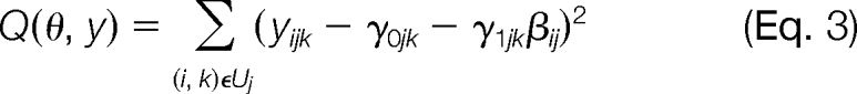
Below, we provide a detailed description of our procedure for obtaining ProPCA estimates. For a fixed protein j, let U_j = {(i, k); y_ijk is observed} be the collection of indices corresponding to the observed (non-missing) PPA measurements, and let

where θ = (γ_0jk, γ_1jk, β_ij)_{j, k}. Then minimizing (Equation 2) is equivalent to minimizing Q(θ, y) over θ. As a tool to assist in minimizing Q(θ, y), define the surrogate data ỹ = (ỹ_ijk)_{(i, k)∉Uj}, where each entry, ỹ_ijk, corresponds to a missing value in the log(PPA) data. Now define the surrogate minimization function as

and note that for fixed ỹ, minimizing Q(θ, ỹ, y) is equivalent to minimizing an instance of Equation 2 with no missing data. In particular, for fixed ỹ, Q₀(θ, ỹ, y) can be minimized in a computationally efficient manner and is equivalent to finding the first principle component corresponding to the data comprising both the observed data, y, and the surrogate data, ỹ. The majorization-minimization algorithm for optimizing (Equation 2) and obtaining ProPCA estimates is an iterative procedure, which proceeds as follows. The surrogate data for the first step of the algorithm is y⁽⁰⁾ = (0)_{(i, k)∉Uj}. Given surrogate data for the rth step, y^{(r − 1)} = y_{ijk (i, k)∉Uj}^{(r − 1)} (with r ≥ 1) let

be the minimizer of Q₀(θ, y^{(r − 1)}, y). Define the surrogate data for the (r + 1)th step, y^(r) = (y_ijk^(r))_{(i, k)∉Uj}, by y_ijk^(r) = γ̂_0jk^(r) + γ̂_1jk^(r)β̂_ij^(r). Iterate until ‖y^(r) − ^{y(r − 1)}‖ is small, and return β̂_j^(r) = (β̂_ij^(r))_{i = 1}^N after the last iteration; β̂_j^(r) is the ProPCA estimate for the jth protein. This algorithm is easily implemented, and in our experience, computation time is minimal.

HepG2 Sample Preparation

Human hepatocellular carcinoma cells were grown in minimum Eagle's medium with 10% FBS in two separate 10-cm dishes to 90% confluence. The cells in each plate were washed with chilled PBS and harvested separately in 1.0 ml of lysis buffer containing 8 m urea, 50 mm NaCl, 50 mm ammonium bicarbonate, pH ∼8.0, 5 mm tris(2-carboxyethyl)phosphine hydrochloride (TCEP) as well as protease and phosphatase inhibitors (Complete Mini tablets (Roche Applied Science), 1 mm NaF, 1 mm β-glycerophosphate, 1 mm sodium orthovanadate, 10 mm sodium pyrophosphate, 1 mm PMSF, 2 mm CaCl₂). The lysis buffer used for plate 2 also contained 30% 1,1,1,3,3,3-hexafluoro-2-propanol (heptafluoroisopropanol (HFIP)). The cells were scraped and collected in 15-ml conical tubes. The cells were lysed in an ultrasound bath at 0 °C for 15 min and then vortexed for 1 min. Each lysate was centrifuged at 4,000 rpm for 5 min at 4 °C to spin down cell debris. The volume was brought to 2.5 ml with 50 mm ammonium bicarbonate, and TCEP was added to 5 mm. The lysates were vortexed and incubated for 15 min at 56 °C to reduce remaining disulfide bonds and then cooled to room temperature. Iodoacetamide was added to 10 mm, and the lysates were vortexed and incubated for 30 min at room temperature in the dark. To quench excessive iodoacetamide, TCEP was added to a concentration of 5 mm and incubated for 15 min in the dark at 37 °C. The lysates were diluted 5-fold with 25 mm ammonium bicarbonate, pH 8.6. Six 20-μl aliquots of the resulting lysates were transferred to polypropylene Eppendorf tubes and subjected to overnight tryptic digestion. 0.3 μg of trypsin (Promega) was added to each tube to achieve an enzyme/substrate ratio of ∼1:70–1:100. Formic acid was added to 1% (v/v) to quench enzymatic action. Samples were vacuum-concentrated to 5 μl and then resuspended to a total volume of 44 μl in 2% formic acid, 2% acetonitrile. The samples were centrifuged for 15 min at 10,000 rpm and transferred to autosampler vials. The resulting digests were analyzed by one-dimensional nano-LC-ESI-tandem mass spectrometry as described above.

Software Availability

The R code for implementing ProPCA, given log(SC) and log(PPA) data, is included in the supplemental data and is available at http://www.hsph.harvard.edu/proteomics/software.

RESULTS

Protein Standards

The data set used to validate the performance of ProPCA was derived from the LC-MS/MS analysis of fractions of the UPS2 proteomic dynamic range standard set² (manufactured by Sigma-Aldrich). The UPS2 standard set contains 48 proteins with a dynamic range of 5 orders of magnitude, spanning 0.5–50,000 fmol, according to the manufacturer. The various fractions used in our analysis each contained one of 11 specified amounts of the UPS2 standard, determined by a number η, and spanned over 2 orders of magnitude (supplemental Table S2). Overall, data from 38 LC-MS/MS runs were available for the UPS2 standards, and the analyzed fractions of the UPS2 standard spanned a protein dynamic range of more than 7 orders of magnitude.

Data Processing Step

ProPCA relies on SCs and PPA measurements that must be extracted from the raw LC-MS/MS data. Several software platforms that perform this are available. We used SEQUEST and PeptideProphet (30) to identify peptides and proteins by MS and MS/MS spectra and to obtain SCs. In our analysis of the UPS2 data, 305 distinct peptides corresponding to 22 of the 48 known proteins in the UPS2 standard set were identified (no up-front fractionation techniques or long LC gradients were used to enhance sensitivity across a wider dynamic range because this was not the primary goal of this study). The 22 identified proteins were higher abundance proteins in the UPS2 standard set with abundances ranging from 500 to 50,000 fmol (supplemental Table S1). To obtain PPA measurements for our primary analysis, we used msInspect/AMT (17, 18), which, in turn, identifies LC-MS peaks, calculates peptide peak areas (by integrating LC-MS peaks over the scan domain), aligns peaks from several analyses, and matches these to identified peptides. We refer to the generic procedure where one begins with raw LC-MS/MS data and ultimately obtains SCs and PPA measurements as the data processing step.

For each protein, the data relevant for ProPCA may be represented as a matrix. Such a matrix is found in Table I, which contains spectral count and PPA information about the protein cytochrome b₅ for several randomly selected LC-MS/MS runs from the UPS2 standard data set. In fact, a data matrix with 38 rows, one for each LC-MS/MS run in the UPS2 data set, is available for cytochrome b₅, and this larger matrix was used in our statistical analysis; Table I is offered only as a conceptual aide (data matrices for all proteins from all runs for both the UPS2 and HepG2 experiments are available in the supplemental data in the form of .tsv files and R list objects, which may be easily manipulated with the R statistical software (http://www.r-project.org)). Missing entries in Table I indicate that the PPA measurement procedure was unable to find a PPA corresponding to the appropriate peptide in the given sample. This may be because the peptide is not present in the sample or because of deficiencies in the PPA measurement method. On the other hand, in a number of samples (e.g. samples 1, 4, and 10), PPA measurements are available for certain peptides, yet the SC is 0. This occurs when there are no MS/MS identifications in the sample, yet peak matching software is able to match and quantify peaks based on information from other samples. Given the data in Table I, the goal of any peptide-protein roll-up procedure is to combine SCs and PPA measurements into a single number for each sample that reflects protein abundance.

Table I. Spectral counts and PPA information for cytochrome b₅ (UniProt accession number P00167) from several representative LC-MS/MS runs.

LC-MS/MS run no.	ηa	SCb	TFIIGELHPDDRPKc	VYDLTK	YYTLEEIQK	FLEEHPG	ISAVAVALMYR	STWLILLHK
1	0.0002	0	4.54e + 04	—d	—	—	—	2.63e + 04
4	0.0002	0	4.93e + 04	—	1.69e + 04	—	—	5.78e + 03
9	0.0004	1	—	3.31e + 05	5.02e + 04	3.01e + 05	—	—
10	0.0004	0	1.58e + 05	3.65e + 05	5.24e + 04	3.08e + 05	—	—
23	0.002	3	1.60e + 06	2.14e + 06	3.69e + 05	1.69e + 06	1.73e + 04	—
29	0.01	8	1.12e + 07	1.14e + 07	1.92e + 06	1.01e + 07	2.34e + 05	4.49e + 06
36	0.03	5	1.27e + 07	2.62e + 07	4.04e + 06	2.36e + 07	9.07e + 05	1.28e + 07
38	0.03	7	3.54e + 07	2.83e + 07	5.71e + 06	2.78e + 07	—	1.50e + 07

^a Relative protein abundance; see supplemental Table S1.

^b Spectral count.

^c The fourth through ninth columns correspond to peptides matched to cytochrome b₅ in the UPS2 LC-MS/MS data set; the name of each of these columns indicates the amino acid sequence of the peptide.

^d Missing PPA measurements are signified by “—.”

Normalization

Various normalization techniques may be utilized to transform the LC-MS/MS data described above to the appropriate scale and address potential artifacts in the data. Previous work has noted that the logarithm of SCs is highly correlated with the logarithm of protein abundance (7, 8), and this is consistent with our observations. Indeed, let log(SC) denote the natural logarithm of SCs (before taking logarithms, we added 1 to each SC to avoid taking the logarithm of 0); the mean of sample correlation coefficients between log(SC) and log protein abundance, taken over all proteins identified in the UPS2 standards, was 0.81 ± 0.13 (mean ± S.D.). We point out that other earlier work has indicated that untransformed SCs are correlated with the logarithm of protein abundance (6) (linear-log relationship) or untransformed protein abundance (5) (linear-linear relationship). In our analysis, we found good correlation on the linear-log scale (mean ± S.D., 0.82 ± 0.15). However, correlation on the linear-linear scale was substantially lower (mean ± S.D., 0.60 ± 0.20); this may be due to the wide dynamic range in the UPS2 standard set.

Upon examination of PPA measurements, we found that the natural logarithms of PPA measurements, denoted log(PPA), are highly correlated with the logarithm of protein abundance (mean sample correlation coefficient across peptides identified in UPS2 standards ±S.D., 0.92 ± 0.20) and that the logarithms of PPA measurements are nearly normally distributed when compared with the raw PPA measurements (supplemental Fig. S1). Fig. 1 depicts scatter plots of log protein abundance versus log(SC) and log(PPA) for a few representative proteins and peptides; the supplemental data contain similar plots for all identified peptides and proteins in the UPS2 standards. Given these observations about correlation in SCs and PPA measurements, we recommend applying a logarithm to both SCs and the PPA data. Below, we work exclusively with log(SC) and log(PPA).

Fig. 1.

Correlation with log protein abundance. Rows a–c, scatter plots of log protein abundance, denoted log(η) (supplemental Table S1), versus ProPCA, log(SC), and ProALT for three representative proteins from the UPS2 standard set (UniProt accession numbers P41159, P62937, and P06732). The sample correlation coefficient is noted under each plot. Row d, scatter plots of log(η) versus log(PPA) for three representative peptides from the UPS2 standard set (based on msInspect/AMT PPA measurements; amino acid sequences HDTSLKPISVSYNPATAK, LKPLSVSYDQATSLR, and DMQLGR).

In addition to applying log transformations to the data, it may be desired to normalize SCs and peptide peak areas within samples and across samples. Normalizing within samples (9, 31–33) is advisable if the quantity of interest is the abundance of a given protein relative to sample total protein abundance or to the abundance of certain housekeeping proteins in a biological sample. In our UPS2 standard set, we did not normalize within samples because, as part of the experimental procedure, different samples contained different amounts of the protein mixture. We did not normalize within samples in the cell lysate data because, at the experimental stage, samples were standardized to contain cell lysate from an equal number of HepG2 cells. Furthermore, in the HepG2 cell lysate data, per-sample overall protein abundance is a quantity of scientific interest.

Normalizing across samples may be performed to match the distributions of SCs and peptide peak attribute measurements. This is a reasonable goal given our task of combining disparate indicators of protein abundance. However, in our experience with ProPCA and the other methods for peptide-protein roll-up discussed below, we have found that normalizing across samples tends to attenuate observable differences in protein abundance. For example, one reasonable approach is, for each protein, to normalize log(SC) and the log(PPA) measurements of each peptide so that they have equal means and equal standard deviations. After normalizing in this manner, we found that the association between ProPCA and log protein abundance decreased in the UPS2 standard set when compared with the non-normalized data; we also observed a decrease in association with log protein abundance when alternative peptide-protein roll-up procedures were used (supplemental Table S3). We conjecture that the observed decrease in association when utilizing normalized data may be due to the substantial missingness in PPA measurement data and difficulties in approximating population-level means and standard deviations. Ultimately, we did not normalize across samples in our analysis described below. However, further research into normalization techniques for ProPCA and other peptide-protein roll-up procedures may be fruitful.

ProPCA

Spectral counting and PPA-based methods for protein quantification are driven by the observation that these measurements are correlated with protein abundance on an appropriate scale. As discussed above, in the UPS2 standards, log(SC) and log(PPA) were both highly correlated with log protein abundance. ProPCA estimates are derived by formalizing the assumption that log(SC) and log(PPA) vary linearly with the logarithm of protein abundance. ProPCA is an unsupervised method for the estimation of relative protein abundance. In the complete data case, the ProPCA estimates for a given protein are equal to the first principal component (22) of the protein data matrix. When PPA measurements are missing, ProPCA estimates are obtained using a majorization-minimization algorithm (27). Ultimately, ProPCA provides an estimate of the relative protein abundance of each identified protein in each sample. As with many PCA-based procedures, training data containing known protein abundances are not required to implement ProPCA. Additionally, ProPCA estimates are only defined up to an affine transformation. In the absence of additional information, this may be problematic in attempts to estimate absolute protein abundance. However, because of the invariance of many common statistical tests to affine transformations (e.g. t tests), this ambiguity is largely irrelevant for detecting whether a given protein is differentially abundant across samples.

In addition to estimates of relative log protein abundance, the ProPCA procedure allows one to determine the spectral count and peptide coefficients, γ̂_1jk (the minimizers of Equation 2). In the complete data setting where ProPCA is equivalent to principal component analysis, these coefficients indicate the relative contribution of spectral counts and the various peptides to the ProPCA estimator: larger coefficients indicate that spectral counts or the corresponding peptide play a larger role in determining the ProPCA estimator. With missing data, the interpretation of γ̂_1jk is less straightforward; however, the coefficients may still offer some insight into the role spectral counts and each peptide plays in determining the ProPCA estimator. The coefficients γ̂_1jk for the UPS2 standard data are plotted in supplemental Fig. S2 and Table S4.

Below, we compare the performance of ProPCA with that of SCs and an existing peptide-protein roll-up method that utilizes only PPA measurements. This PPA-based roll-up procedure was described by Jaffe et al. (16). Referred to as ProALT (for alternative protein roll-up) estimates, these protein-level estimates are obtained by first dividing each log(PPA) measurement by the maximum observed log(PPA) measurement for the peptide under consideration to obtain adjusted peptide measurements. Samples where a peptide was not observed are then taken to have adjusted peptide measurement equal to 0. Protein level estimates for each sample are found by taking the mean value of all corresponding adjusted peptide measurements.

Association

The sample correlation coefficient between log protein abundance and ProPCA, log(SC), and ProALT estimates was computed for each identified protein in the UPS2 standards. The mean sample correlation coefficient between ProPCA estimates and log protein abundance ±S.D. was 0.97 ± 0.05. For log(SC) and ProALT, the mean sample correlation coefficient with log protein abundance ±S.D. was 0.81 ± 0.13 and 0.86 ± 0.11, respectively. It appears that ProPCA estimates have substantially higher correlation with log protein abundance than log(SC) and ProALT estimates. Plots of the various estimates versus log protein abundance for several representative proteins are found in Fig. 1; the supplemental data contain plots for all identified proteins in the UPS2 standards.

Power

High correlation with the logarithm of protein abundance indicates the predictive ability of ProPCA estimates. Predicting absolute protein abundances or even relative abundances that are comparable across proteins as well as samples remains challenging and requires additional, non-trivial normalization procedures that we do not discuss in here (8). Rather, we focus on the application of ProPCA estimates to detecting the differential abundance of a given protein between two groups.

We evaluated the power of each estimation procedure, ProPCA, log(SC), and ProALT, to distinguish between samples with different protein abundances when used in conjunction with t tests. Using ProPCA, log(SC), and ProALT estimators, we conducted t tests comparing UPS2 samples with different protein abundances. These tests were performed for each protein identified in the UPS2 standard data set and each pair of differing abundances. Because protein abundances were known to differ between compared samples, each t test would ideally return a significant p value. Furthermore, the frequency of significant t tests is an indicator of the power of an estimation method to distinguish between samples with different protein abundance. In fact, a more nuanced picture of the performance of an estimation method may be obtained by studying the distribution of p values obtained in this manner (Fig. 2) as opposed to simply the number of those that are below 0.05 or some other significance threshold: in this setting, a better estimation procedure should have smaller p values. The procedure is described in more detail in the following paragraph.

Fig. 2.

Estimated power versus putative type 1 error rate (α) with validation (msInspect/AMT PPA measurements). a, the estimated power of a given method, controlling for a putative type 1 error rate (size) of α, is the proportion of p values less than α. At α = 0.05, the estimated power of ProPCA, log(SC), and ProALT is 0.82, 0.50, and 0.53, respectively. ProPCA has greater power than log(SC) across the entire range of α and greater power than ProALT across nearly the entire range of α (ProALT has slightly greater power than ProPCA for values of α very close to 1; however, power results for values of α close to 1 tend to be uninteresting because they correspond to tests with very high false positive rates). To validate the results in a, the data were permuted, and we performed t tests on random, indistinguishable groups of samples. A properly calibrated procedure should return p values that are nearly uniformly distributed. b, cumulative distribution of p values; for uniformly distributed p values, we expect to see a line of slope 1 through the origin. In particular, we expect 5% of all p values to be less than 0.05. We found 4.7, 5.1, and 4.7% of p values below 0.05 for ProPCA, log(SC), and ProALT, respectively; all of these values are near 5%. c–e, histograms of p values for ProPCA, log(SC), and ProALT. These results indicate that the permutation-based p values are nearly uniformly distributed.

For a given pair of the 11 distinct abundances among the analyzed fractions of the UPS2 standards, say (η₁, η₂) where η₁ ≠ η₂ (see supplemental Table S1), and each of the 22 identified proteins, we computed ProPCA, log(SC), and ProALT estimates of log protein abundance based on all samples with protein amount η₁ or η₂. Then, we performed t tests for each estimation method and each identified protein, comparing samples with protein level η₁ with those with level η₂. We declared a t test with associated p value less than 0.05 to be significant. Because η₁ ≠ η₂, an ideal protein abundance estimator would always return a significant t test. This procedure was repeated for all pairs of distinct protein levels in the UPS2 standards. In total, 1210 (=22 × 11 × 10/2) t tests were conducted for each of the three procedures. We computed the percentage of significant t tests for each estimation methods and found that t tests based on ProPCA estimates were significant in 82% of tests; 50 and 53% of t tests were significant for log(SC) and ProALT, respectively.

Fig. 2a indicates that ProPCA when used with t tests is rather successful at identifying differentially abundant proteins in the UPS2 standards, especially when compared with log(SC) and ProALT. In general, the appropriateness of t tests may be suspect if the data do not follow a normal distribution (34). As discussed above and depicted in supplemental Fig. S1, by working with log(PPA), measurements were more closely normally distributed. However, the ProPCA, log(SC), and ProALT data were still decidedly non-normal as indicated by the Shapiro-Wilk test for normality (35) (p values for ProPCA, log(SC), and ProALT are all below 10⁻¹⁰). On the other hand, in our analysis of the performance of ProPCA, we were not inherently interested in the testing procedure; rather, we were primarily interested in the reliability of p values obtained from the testing procedure and the relative performance of ProPCA as compared with log(SC) and ProALT. Although the data may not be exactly normally distributed, this does not necessarily render the p values obtained from t tests useless. Indeed, if the p values obtained from t tests comparing hypothetical groups with the same average protein abundance are uniformly distributed on the interval [0, 1], that is, if the p value distribution is uniform on [0, 1] under the null hypothesis, then the p values are valid regardless of distributional assumptions about the data. To validate the p values in Fig. 2a, we used a permutation method to approximate the null distribution of p values, and we showed that this distribution is approximately uniform on [0, 1] (Fig. 2, b–e). More specifically, for each identified protein in the UPS2 standards, we randomly assigned each of the 38 samples and the corresponding protein abundance estimates (ProPCA, log(SC), and ProALT estimates) to one of two groups. We then conducted t tests for each identified protein and each estimation method, comparing the two randomly constructed groups. We repeated this procedure 1000 times, each time randomly creating two groups for comparison. Thus, in total, 22,000 t tests were conducted for each estimation method. Because samples are randomly assigned to groups, we expect that on average there is no difference between the two groups. Fig. 2, b–e, indicate that the p value distribution for each estimation method is very close to uniform on the interval [0, 1]. This suggests that our power analysis in Fig. 2a is sound.

We do not broadly advocate the use of t tests with LC-MS/MS data. Non-normality of the data and a lack of replicates, which is common in LC-MS/MS data, complicates the matter, and in any given situation, an alternative to t tests may be more appropriate (36). In fact, ProPCA estimates may be used in conjunction with any procedure for the statistical analysis of relative protein abundance that utilizes a continuous outcome. However, given that t tests appear to provide credible results with the UPS2 standard data, we believe that the t test is a reasonable method for illustrating the performance of ProPCA estimates because of its simplicity. Because ProPCA estimates are more highly associated with log protein abundance than their competitors, as described in the previous section, we believe that our results using t tests offer a reliable indication of the comparative performance of ProPCA, log(SC), and ProALT when used with more specialized methods.

It should be noted that ProPCA should not be used in conjunction with the G test (31) or other procedures that rely on discrete outcomes (9); however, for most discrete outcome procedures, a continuous outcome analog is available at least in principle (for instance, a general likelihood ratio test for continuous outcomes (37) may be used in place of the G test and hierarchical models (38) to provide a continuous outcome analog of the methods proposed by Choi et al. (9)).

Above, we have essentially implemented a bootstrap method (39) to estimate the power of ProPCA. An alternative approach to estimating power is via simulation. We prefer the bootstrap approach because of the difficulties associated with accurately simulating LC-MS/MS proteomics data; furthermore, our bootstrap approach more fully utilizes the available data.

Low Match Rates

In the UPS2 data, the msInspect/AMT procedure was successful in the sense that peptides identified by MS/MS spectra were matched to corresponding peaks in the LC-MS domain at a relatively high frequency. In our data set of the UPS2 standards, the msInspect/AMT match rate was 43%, whereas in the HepG2 cell lysate data (discussed below), the match rate was 17% (the match rate was calculated by dividing the total number of msInspect/AMT matches to peptide ion LC-MS peaks by the product of the total number of samples and the total number of peptides identified by MS/MS spectra; this number was then multiplied by 100 to obtain a percentage). The lower match rate in the HepG2 data was expected and likely due to the greater complexity of unfractionated cell lysates.

To study the performance of ProPCA under lower match rates in a simulated setting, we randomly deleted PPA measurements from the UPS2 standard data set to approximate prespecified match rates below 43% (the full match rate). We obtained 100 data sets with equally spaced match rates ranging between 4 and 43%. For each of these 100 data sets and each estimation method, we performed t tests on pairs of protein abundance levels, as discussed in the previous section, to estimate the power of ProPCA at various match rates. We also performed the permutation testing method discussed above with each low match rate data set to validate the power results. Our results suggest that ProPCA outperforms log(SC) and ProALT over nearly the entire range of match rates, giving a significant improvement in power while maintaining a type 1 error rate very close to the putative value (at very low match rates, match rates below that of the HepG2 cell lysate data, log(SC) may outperform ProPCA). Results are summarized in Fig. 3.

Fig. 3.

ProPCA and low match rate data. a, ProPCA, log(SC), and ProALT estimators were computed for each of 100 low match rate data sets, and t tests were performed, as in Fig. 2, to estimate the power of each procedure. Estimated power of each estimation procedure, controlling for a type 1 error rate of 0.05, is plotted versus match rate (non-bold points). These results indicate that ProPCA outperforms log(SC) at all but the lowest match rates and that ProPCA outperforms ProALT over the entire range of match rates. The estimated power of log(SC) remains constant across all match rates because, in this analysis, SCs do not change with match rate. Bold points denote the fraction of significant t tests at the 0.05 level and match rate in the HepG2 cell lysate data. For the HepG2 data, 52, 49, and 24% of t tests corresponding to ProPCA, log(SC), and ProALT, respectively, were significant at the 0.05 level, and the match rate was 17%. b, to validate the results in a, t tests were performed on permuted data (similar to Fig. 2). The proportion of significant t tests (at the 0.05 level) are plotted versus various match rates. A properly calibrated test should have a significance rate of 0.05. These results suggest that the t tests in a were properly calibrated over a wide range of match rates. However, when the match rate is very low, the significance rates for ProALT are especially low. This may occur because ProALT relies entirely on PPA measurement data, which deteriorate as the match rate decreases.

Our procedure for generating data with low match rates may not accurately mimic the missingness mechanism governing the msInspect/AMT matching procedure (40); however, we believe that our results may offer insight into the performance of ProPCA. Further study and additional modeling of missingness, although challenging, could prove fruitful in the analysis of the performance of ProPCA. On the other hand, with additional modeling comes the risk of high sensitivity to violations of the modeling assumptions. Given the complexity of LC-MS/MS data, one should be mindful of this.

Alternative PPA Measurements

To determine the robustness of ProPCA to the data processing step, we used Progenesis LC-MS software (Nonlinear Dynamics) to obtain alternative PPA measurements from the raw UPS2 standard data set. Using the resulting PPA measurement data and the SC data obtained in our primary analysis, we computed log(SC), ProALT, and ProPCA estimates. The mean sample correlation coefficient of ProPCA, log(SC), and ProALT estimates with log protein abundance ±S.D. was 0.88 ± 0.14, 0.81 ± 0.13, and 0.80 ± 0.19, respectively. We performed power calculations and permutation tests similar to those discussed above; the results are displayed in Fig. 4. Overall, the results using Progenesis LC-MS PPA measurements were similar to the results of our primary analysis using msInspect/AMT PPA measurements: ProPCA outperformed log(SC) and ProALT. However, the performance gap was not as large.

Fig. 4.

Estimated power versus putative type 1 error rate (α) with validation (Progenesis PPA measurements). a, power results for Progenesis PPA measurement data (as in Fig. 2). At α = 0.05, the estimated power of ProPCA is 0.60, the estimated power of log(SC) is 0.53, and the estimated power of ProALT is 0.47. Overall, ProPCA appears to outperform log(SC) and ProALT; however, the margin is not as large as in Fig. 2 where msInspect/AMT PPA measurements are utilized. This may be because log(PPA) measurements from the Progenesis software were not as highly correlated with log protein abundance as those from msInspect/AMT (see “Alternative PPA Measurements” under “Results”). b–e, permutation test results for Progenesis PPA measurement data (as in Fig. 2). The p value distributions appear to be nearly uniform, suggesting that the testing and estimation procedures are properly calibrated.

The relatively small gains of ProPCA over log(SC) and ProALT when using the Progenesis LC-MS software compared with those observed when using msInspect/AMT were likely due to the fact that log(PPA) measurements from the Progenesis LC-MS software were not as highly correlated with log protein abundance as those from msInspect/AMT. Indeed, for the Progenesis LC-MS data, the mean sample correlation coefficient between ProPCA estimates and log protein abundance ±S.D. was 0.88 ± 0.14). For log(SC) and ProALT, the mean sample correlation coefficient with the logarithm of protein abundance ±S.D. was 0.81 ± 0.13 and 0.80 ± 0.19, respectively. Note that the results for log(SC) are the same as in the primary analysis where msInspect/AMT was used to find PPA measurements. This is because we used the same procedure to obtain SCs in both analyses. On the other hand, the mean sample correlation coefficients for ProPCA and ProALT estimates were both lower than in the primary analysis using the msInspect/AMT data. This is possibly explained by the fact that overall the correlation between log(PPA) measurements and log protein abundance is lower for the Progenesis data. Recall that in the msInspect/AMT data the mean sample correlation coefficient between log(PPA) and log protein abundance ±S.D. was 0.92 ± 0.20. In the Progenesis data, the mean sample correlation coefficient between log(PPA) and log protein abundance ±S.D. was 0.83 ± 0.26 where the mean is taken over all peptide-specific sample correlation coefficients. We also computed sample correlation coefficients between the untransformed PPA measurements and protein abundance to determine whether the original (non-logarithmic) scale was more appropriate for the Progenesis data. The mean sample correlation coefficient between the untransformed PPA measurements and protein abundance ±S.D. was 0.87 ± 0.31, which is not substantially different from the mean sample correlation coefficient between log(PPA) and log protein abundance.

Application of ProPCA to Analysis of Human Hepatocellular Carcinoma HepG2 Cell Lysate Data

Having assessed the performance of ProPCA in comparison with two other methods, we now discuss application of ProPCA to the results of LC-MS/MS analysis of total HepG2 cell lysates. Equal numbers of human hepatocellular carcinoma HepG2 cells were lysed using two different procedures and prepared for LC-MS/MS analysis. In one procedure, the urea-based lysis buffer contained 30% HFIP; in the other procedure, no HFIP was used. Other than this distinction, the two procedures were identical. Heptafluoroisopropanol, a highly polar, strong organic solvent miscible with water, was applied to facilitate the dissolution of cells, micelles, and membrane fragments and to increase the efficiency of hydrophobic protein recovery (41). After analysis by LC-MS/MS, SCs were computed, and msInspect/AMT was used to obtain PPA measurements. In total, data from six LC-MS/MS runs were available (three replicate runs from each preparation method).

In the HepG2 cell lysate data, 1283 peptides and 407 proteins in total were identified by tandem MS spectra across all six runs; additionally, 10,202 spectral counts were tabulated. Table II contains a run-by-run summary of spectral counts and peptide and protein information for the HepG2 cell lysate data. Before applying ProPCA or other protein abundance estimation procedures, we note that insight into overall protein recovery may be gained by considering total spectral counts, peptide identification, and protein identification information for the two preparation methods. In the data corresponding to runs where HFIP-assisted lysis was utilized, the average number of spectral counts tabulated, peptides identified, and proteins identified ±S.D. was 1822.33 ± 103.12, 682.67 ± 46.37, and 306.67 ± 14.74, respectively. In the data corresponding to runs where conventional lysis without HFIP was utilized, the average number of spectral counts tabulated, peptides identified, and proteins identified ±S.D. was 1713.00 ± 33.45, 616.33 ± 27.57, and 265.33 ± 8.39, respectively. These results indicate that, overall, higher protein content is recovered by LC-MS/MS analysis of samples prepared with the assistance of HFIP. Especially among the runs where conventional lysis was utilized, standard deviations across replicates corresponding to spectral counts, peptides identified, and proteins identified were relatively small and indicated good run-to-run analytical reproducibility. A sizeable fraction of proteins identified in at least one technical replicate were in fact identified in all three technical replicates for each preparation method: 74.00% of all proteins identified in the HFIP-assisted runs were identified in all three replicates, and 65.30% of all proteins identified in the conventional lysis runs were identified in all three replicates. The corresponding numbers for peptide identification were not as high: 53.70% of all peptides identified in the HFIP-assisted lysis runs were identified in all three replicates, and 53.74% of all peptides identified in the conventional lysis runs were identified in all three replicates. We suspect that these percentages would be higher had prefractionation techniques been utilized in these experiments.

Table II. Summary of spectral counts and peptide and protein information for HepG2 cell lysate data.

Run ID/replicate	No. spectral counts	No. peptides	No. proteins
HFIP-assisted lysis
1	1704	632	293
2	1870	693	315
3	1893	723	321
Mean ± S.D.	1822.33 ± 103.12	683.67 ± 46.37	309.67 ± 14.74
Conventional lysis
1	1751	645	275
2	1688	590	261
3	1700	614	260
Mean ± S.D.	1713 ± 33.45	616.33 ± 27.57	265.33 ± 8.39

We computed ProPCA, log(SC), and ProALT protein abundance estimates for each identified protein and used t tests to identify proteins that were differentially recovered from the cells. Although using more refined alternatives to t tests for detecting differences in protein abundance may be of interest in the present setting, we used t tests as opposed to a more involved procedure to highlight the utility of ProPCA, especially as compared with log(SC) and ProALT. Additionally, we point out that the sample correlation coefficient between across-replicate means and standard deviations of ProPCA estimates was very low (−0.016) when computed using all identified proteins in the HepG2 data set. This is notable because high correlation between these means and standard deviations is one motivation for some alternatives to t tests (36, 42). Using ProPCA, 210 of the 407 proteins were found to be significant at the 0.05 level. Using log(SC) and ProALT, 201 and 98 proteins were found to be significant at the 0.05 level, respectively. Thus, as with the UPS2 standards, ProPCA identifies more proteins with p value below 0.05 than the two alternatives. These results do not account for multiple comparisons (also referred to as “multiple testing”), which are important when a large number of comparisons are made. To adjust for multiple testing, we performed the Benjamini-Hochberg (43) “step up” procedure to identify significant proteins and preserve a false discovery rate (FDR) of 5%. Other approaches to adjust for multiple testing, such as the Bonferroni correction (34), control the probability of making any false discoveries (the family-wide error rate) rather than controlling the proportion of false discoveries; this tends to be overly conservative. The Benjamini-Hochberg procedure, on the other hand, is a widely used and easily implemented statistical method for controlling the FDR at a specified level.

Using the Benjamini-Hochberg procedure, 102, 85, and 68 proteins were found to be significant using ProPCA, log(SC), and ProALT, respectively. Although ProPCA finds many more significant proteins at the specified thresholds, we found that ProALT obtains a greater number of extremely small p values than ProPCA (the smallest ProPCA p value is 5.24 × 10⁻⁵, and 10 ProALT p values are smaller than this). This may be related to the low match rate and missingness patterns in the cell lysate data and merits further investigation (recall that the match rate in the HepG2 data was 17%). Despite this observation, we believe these results indicate that ProPCA has more power to detect differentially recovered proteins than its competitors. We conjecture that with higher PPA match rates ProPCA would show greater performance gains over log(SC) and ProALT. This conjecture is supported by our analysis of the UPS2 standards.

As discussed above, the results in Table II suggest that the HFIP lysis method may lead to the recovery of more proteins by LC-MS/MS analysis than the conventional lysis method. Moreover, the ProPCA results suggest that the different lysis techniques (with HFIP or without) lead to the recovery of somewhat different sets of proteins. To better understand the differences in protein recovery enabled by each lysis approach, we performed an exploratory gene ontology (GO) term enrichment analysis by means of the MetaCore software suite (GeneGO, St. Joseph, MI) using the significant proteins identified by ProPCA (those that were significant at a 5% FDR according to the Benjamini-Hochberg method). Significantly enriched gene ontology cellular localization terms were identified, and the most prominent terms are found in Fig. 5. It appears that the addition of HFIP into the lysis buffer leads to improved recovery of membrane-associated proteins; proteins of various macromolecular complexes; cytoskeleton-associated, ribosomal, and nuclear proteins; and proteins of other organelles in addition to superior recovery of cytosolic proteins. We attribute this enrichment of hydrophobic as well as membrane- and complex-associated proteins to the ability of HFIP to form strong hydrogen bonds and bind with and dissolve cellular molecular formations incorporating receptive moieties, such as amino groups, amides, oxygen, and double bonds. Interestingly, mostly mitochondrial proteins and some cell adhesion/cell motility as well as complex-forming proteins were better extracted using the conventional urea-based lysis buffer without the addition of the acidic fluoroalcohol. Although elucidation of grounds for this phenomenon would require supplementary experiments, we did expect that the addition of hexafluoroalcohol would not result in overall improvement of protein solubility because proteome constituents exhibit vastly different physical and chemical properties. Nevertheless, the ProPCA analysis supports the notion of possible targeted tune-up of cell or tissue lysis conditions to recover certain proteins of interest more efficiently.

Fig. 5.

Functional characterization of HepG2 proteomes differentially recovered using alternative cell lysis methods. Proteins that exhibited significant differential recovery (enrichment) in the HepG2 data (FDR, 5%) were segregated into two groups: one containing proteins that appeared to be more enriched in the conventional lysis data and the other containing proteins that appeared to be more enriched in the HFIP lysis data (this determination was based upon the sign of the associated t statistics). The two lists were analyzed separately using the GeneGO software suite. Each analysis produced a list of significant GO localization terms and associated p values. GO localization terms with significant differential enrichment in the HepG2 cell lysate experiments are shown. Each bar represents the difference in negative log-transformed p values (−log(p)) of the specific GO localization term. p values indicate enrichment (recovery) of proteins corresponding to each GO term and were determined using the GeneGO software suite. Positive difference scores indicate likely increased enrichment by HFIP-assisted lysis. GO localization terms are arranged so that terms with likely increased enrichment by HFIP-assisted lysis appear at the top of chart; additionally, terms corresponding to similar functional and subcellular organelle association are grouped and colored accordingly: these generalized localization and functional categories are shown on the left side of the figure.

DISCUSSION

Peptide-protein roll-up is an important issue in the analysis of bottom-up LC-MS/MS proteomics data. We have proposed ProPCA, a new method for peptide-protein roll-up, and have shown that ProPCA estimates are more highly correlated with the logarithm of protein abundance than estimates derived using other peptide-protein roll-up procedures. Additionally, we showed that ProPCA has substantially greater power to detect differences in protein abundance between two groups than competing roll-up procedures. In principle, these procedures could be extended to handle more than two groups, and we would expect ProPCA to perform well in this setting too.

In addition to showing the benefits ProPCA in the analysis of the UPS2 standards, we showed that ProPCA identified more significant proteins than other procedures when applied to the HepG2 cell lysate data. Our preliminary experiments with HepG2 cells were performed using relatively small amounts of starting material without applying any prefractionation techniques, which resulted in quantitative characterization of a small fraction of the HepG2 proteome. Scaling up the analogous experiments and enhancing separation platforms in up-front mass spectrometry analysis will undoubtedly allow for more exhaustive profiling of a cellular proteome and more extensive coverage of gene ontology terms. However, in our experience, the inclination for enhanced recovery of the aforementioned protein classes caused by one or another lysis condition will be similar to that detected with ProPCA based on a smaller fraction of the proteome. The preliminary results presented here should contribute to the existing body of research.

ProPCA does not rely on stable isotopic labeling. Indeed, our testing and validation results are derived from label-free proteomics experiments. However, in principle, ProPCA may also be used for peptide-protein roll-up in the analysis of proteomics experiments that utilize stable isotope labeling methods.

REFERENCES

- 1. Aebersold R., Mann M. (2003) Mass spectrometry-based proteomics. Nature 422, 198–207 [DOI] [PubMed] [Google Scholar]
- 2. Domon B., Aebersold R. (2006) Mass spectrometry and protein analysis. Science 312, 212–217 [DOI] [PubMed] [Google Scholar]
- 3. Cravatt B. F., Simon G. M., Yates J. R., 3rd (2007) The biological impact of mass-spectrometry-based proteomics. Nature 450, 991–1000 [DOI] [PubMed] [Google Scholar]
- 4. Kelleher N., Lin H., Valaskovic G., Aaserud D., Fridriksson E., McLafferty F. (1999) Top down versus bottom up protein characterization by tandem high-resolution mass spectrometry. J. Am. Chem. Soc. 121, 806–812 [Google Scholar]
- 5. Liu H., Sadygov R. G., Yates J. R., 3rd (2004) A model for random sampling and estimation of relative protein abundance in shotgun proteomics. Anal. Chem. 76, 4193–4201 [DOI] [PubMed] [Google Scholar]
- 6. Ishihama Y., Oda Y., Tabata T., Sato T., Nagasu T., Rappsilber J., Mann M. (2005) Exponentially modified protein abundance index (emPAI) for estimation of absolute protein amount in proteomics by the number of sequenced peptides per protein. Mol. Cell. Proteomics 4, 1265–1272 [DOI] [PubMed] [Google Scholar]
- 7. Lu P., Vogel C., Wang R., Yao X., Marcotte E. M. (2007) Absolute protein expression profiling estimates the relative contributions of transcriptional and translational regulation. Nat. Biotechnol. 25, 117–124 [DOI] [PubMed] [Google Scholar]
- 8. Schmidt M. W., Houseman A., Ivanov A. R., Wolf D. A. (2007) Comparative proteomic and transcriptomic profiling of the fission yeast Schizosaccharomyces pombe. Mol. Syst. Biol. 3, 79. [DOI] [PMC free article] [PubMed] [Google Scholar]
- 9. Choi H., Fermin D., Nesvizhskii A. I. (2008) Significance analysis of spectral count data in label-free shotgun proteomics. Mol. Cell. Proteomics 7, 2373–2385 [DOI] [PMC free article] [PubMed] [Google Scholar]
- 10. Zybailov B., Coleman M. K., Florens L., Washburn M. P. (2005) Correlation of relative abundance ratios derived from peptide ion chromatograms and spectrum counting for quantitative proteomic analysis using stable isotope labeling. Anal. Chem. 77, 6218–6224 [DOI] [PubMed] [Google Scholar]
- 11. Eng J., McCormack A., Yates J. R., 3rd (1994) An approach to correlate tandem mass spectra data of peptides with amino acid sequences in a protein database. J. Am. Soc. Mass Spectrom. 5, 976–989 [DOI] [PubMed] [Google Scholar]
- 12. Pappin D. J., Hojrup P., Bleasby A. J. (1993) Rapid identification of proteins by peptide-mass fingerprinting. Curr. Biol. 3, 327–332 [DOI] [PubMed] [Google Scholar]
- 13. Wang W., Zhou H., Lin H., Roy S., Shaler T. A., Hill L. R., Norton S., Kumar P., Anderle M., Becker C. H. (2003) Quantification of proteins and metabolites by mass spectrometry without isotopic labeling or spiked standards. Anal. Chem. 75, 4818–4826 [DOI] [PubMed] [Google Scholar]
- 14. Radulovic D., Jelveh S., Ryu S., Hamilton T. G., Foss E., Mao Y., Emili A. (2004) Informatics platform for global proteomic profiling and biomarker discovery using liquid chromatography-tandem mass spectrometry. Mol. Cell. Proteomics 3, 984–997 [DOI] [PubMed] [Google Scholar]
- 15. Cox J., Mann M. (2008) MaxQuant enables high peptide identification rates, individualized ppb-range mass accuracies and proteome-wide protein quantification. Nat. Biotechnol. 26, 1367–1372 [DOI] [PubMed] [Google Scholar]
- 16. Jaffe J. D., Mani D. R., Leptos K. C., Church G. M., Gillette M. A., Carr S. A. (2006) PEPPeR, a platform for experimental proteomic pattern recognition. Mol. Cell. Proteomics 5, 1927–1941 [DOI] [PMC free article] [PubMed] [Google Scholar]
- 17. Bellew M., Coram M., Fitzgibbon M., Igra M., Randolph T., Wang P., May D., Eng J., Fang R., Lin C., Chen J., Goodlett D., Whiteaker J., Paulovich A., McIntosh M. (2006) A suite of algorithms for the comprehensive analysis of complex protein mixtures using high-resolution LC-MS. Bioinformatics 22, 1902–1909 [DOI] [PubMed] [Google Scholar]
- 18. May D., Fitzgibbon M., Liu Y., Holzman T., Eng J., Kemp C. J., Whiteaker J., Paulovich A., McIntosh M. (2007) A platform for accurate mass and time analyses of mass spectrometry data. J. Proteome Res. 6, 2685–2694 [DOI] [PubMed] [Google Scholar]
- 19. Polpitiya A. D., Qian W. J., Jaitly N., Petyuk V. A., Adkins J. N., Camp D. G., 2nd, Anderson G. A., Smith R. D. (2008) DAnTE: a statistical tool for quantitative analysis of -omics data. Bioinformatics 24, 1556–1558 [DOI] [PMC free article] [PubMed] [Google Scholar]
- 20. Griffin N. M., Yu J., Long F., Oh P., Shore S., Li Y., Koziol J. A., Schnitzer J. E. (2010) Label-free, normalized quantification of complex mass spectrometry data for proteomic analysis. Nat. Biotechnol. 28, 83–89 [DOI] [PMC free article] [PubMed] [Google Scholar]
- 21. Katajamaa M., Oresic M. (2005) Processing methods for differential analysis of LC/MS profile data. BMC Bioinformatics 6, 179. [DOI] [PMC free article] [PubMed] [Google Scholar]
- 22. Rencher A. (2002) Methods of Multivariate Analysis, 2nd Ed., Wiley-Interscience, New York, 380–407 [Google Scholar]
- 23. Peng J., Elias J. E., Thoreen C. C., Licklider L. J., Gygi S. P. (2003) Evaluation of multidimensional chromatography coupled with tandem mass spectrometry (LC/LC-MS/MS) for large-scale protein analysis: the yeast proteome. J. Proteome Res. 2, 43–50 [DOI] [PubMed] [Google Scholar]
- 24. Qian W. J., Liu T., Monroe M. E., Strittmatter E. F., Jacobs J. M., Kangas L. J., Petritis K., Camp D. G., 2nd, Smith R. D. (2005) Probability-based evaluation of peptide and protein identifications from tandem mass spectrometry and SEQUEST analysis: the human proteome. J. Proteome Res. 4, 53–62 [DOI] [PubMed] [Google Scholar]
- 25. May D., Liu Y., Law W., Fitzgibbon M., Wang H., Hanash S., McIntosh M. (2008) Peptide sequence confidence in accurate mass and time analysis and its use in complex proteomics experiments. J. Proteome Res. 7, 5148–5156 [DOI] [PMC free article] [PubMed] [Google Scholar]
- 26. Pedrioli P. G., Eng J. K., Hubley R., Vogelzang M., Deutsch E. W., Raught B., Pratt B., Nilsson E., Angeletti R. H., Apweiler R., Cheung K., Costello C. E., Hermjakob H., Huang S., Julian R. K., Kapp E., McComb M. E., Oliver S. G., Omenn G., Paton N. W., Simpson R., Smith R., Taylor C. F., Zhu W., Aebersold R. (2004) A common open representation of mass spectrometry data and its application to proteomics research. Nat. Biotechnol. 22, 1459–1466 [DOI] [PubMed] [Google Scholar]
- 27. Lange K., Hunter D., Yang I. (2000) Optimization transfer using surrogate objective functions. J. Comput. Graph. Stat. 9, 1–20 [Google Scholar]
- 28. Hunter D. R., Lange K. (2004) A tutorial on MM algorithms. Am. Stat. 58, 30–37 [Google Scholar]
- 29. Troyanskaya O., Cantor M., Sherlock G., Brown P., Hastie T., Tibshirani R., Botstein D., Altman R. B. (2001) Missing value estimation methods for DNA microarrays. Bioinformatics 17, 520–525 [DOI] [PubMed] [Google Scholar]
- 30. Keller A., Nesvizhskii A. I., Kolker E., Aebersold R. (2002) Empirical statistical model to estimate the accuracy of peptide identifications made by MS/MS and database search. Anal. Chem. 74, 5383–5392 [DOI] [PubMed] [Google Scholar]
- 31. Old W. M., Meyer-Arendt K., Aveline-Wolf L., Pierce K. G., Mendoza A., Sevinsky J. R., Resing K. A., Ahn N. G. (2005) Comparison of label-free methods for quantifying human proteins by shotgun proteomics. Mol. Cell. Proteomics 4, 1487–1502 [DOI] [PubMed] [Google Scholar]
- 32. Zhang B., VerBerkmoes N. C., Langston M. A., Uberbacher E., Hettich R. L., Samatova N. F. (2006) Detecting differential and correlated protein expression in label-free shotgun proteomics. J. Proteome Res. 5, 2909–2918 [DOI] [PubMed] [Google Scholar]
- 33. Zybailov B., Mosley A. L., Sardiu M. E., Coleman M. K., Florens L., Washburn M. P. (2006) Statistical analysis of membrane proteome expression changes in Saccharomyces cerevisiae. J. Proteome Res. 5, 2339–2347 [DOI] [PubMed] [Google Scholar]
- 34. Rosner B. (2005) Fundamentals of Biostatistics, 6th Ed., Duxbury Press, Belmont, CA, 296–338 and 573–579 [Google Scholar]
- 35. Shapiro S. S., Wilk M. B. (1965) An analysis of variance test for normality (complete samples). Biometrika 52, 591–611 [Google Scholar]
- 36. Pavelka N., Fournier M. L., Swanson S. K., Pelizzola M., Ricciardi-Castagnoli P., Florens L., Washburn M. P. (2008) Statistical similarities between transcriptomics and quantitative shotgun proteomics data. Mol. Cell. Proteomics 7, 631–644 [DOI] [PubMed] [Google Scholar]
- 37. Casella G., Berger R. L. (2002) Statistical Inference, 2nd Ed., Duxbury Press, Pacific Grove, CA, 374–378 [Google Scholar]
- 38. Gelman A., Carlin J. B., Stern H. S., Rubin D. B. (2004) Bayesian Data Analysis, 2nd Ed., Chapman & Hall/CRC, Boca Raton, FL, 120–160 [Google Scholar]
- 39. Davison A. C., Hinkley D. (1997) Bootstrap Methods and their Application, Cambridge University Press, Cambridge, UK [Google Scholar]
- 40. Karpievitch Y., Stanley J., Taverner T., Huang J., Adkins J. N., Ansong C., Heffron F., Metz T. O., Qian W. J., Yoon H., Smith R. D., Dabney A. R. (2009) A statistical framework for protein quantitation in bottom-up MS-based proteomics. Bioinformatics 25, 2028–2034 [DOI] [PMC free article] [PubMed] [Google Scholar]
- 41. Gross V., Carlson G., Kwan A. T., Smejkal G., Freeman E., Ivanov A. R., Lazarev A. (2008) Tissue fractionation by hydrostatic pressure cycling technology: the unified sample preparation technique for systems biology studies. J. Biomol. Tech. 19, 189–199 [PMC free article] [PubMed] [Google Scholar]
- 42. Rocke D. M., Durbin B. (2001) A model for measurement error for gene expression arrays. J. Comput. Biol. 8, 557–569 [DOI] [PubMed] [Google Scholar]
- 43. Benjamini Y., Hochberg Y. (1995) Controlling the false discovery rate: a practical and powerful approach to multiple testing. J. R. Stat. Soc. Ser. B 57, 289–300 [Google Scholar]
Associated Data
This section collects any data citations, data availability statements, or supplementary materials included in this article.