Analysis of Operating Principles with S-system Models

Abstract

Operating principles address general questions regarding the response dynamics of biological systems as we observe or hypothesize them, in comparison to a priori equally valid alternatives. In analogy to design principles, the question arises: Why are some operating strategies encountered more frequently than others and in what sense might they be superior? It is at this point impossible to study operation principles in complete generality, but the work here discusses the important situation where a biological system must shift operation from its normal steady state to a new steady state. This situation is quite common and includes many stress responses. We present two distinct methods for determining different solutions to this task of achieving a new target steady state. Both methods utilize the property of S-system models within Biochemical Systems Theory (BST) that steady-states can be explicitly represented as systems of linear algebraic equations. The first method uses matrix inversion, a pseudo-inverse, or regression to characterize the entire admissible solution space. Operations on the basis of the solution space permit modest alterations of the transients toward the target steady state. The second method uses standard or mixed integer linear programming to determine admissible solutions that satisfy criteria of functional effectiveness, which are specified beforehand. As an illustration, we use both methods to characterize alternative response patterns of yeast subjected to heat stress, and compare them with observations from the literature.

Introduction

Biological design principles refer to structural or regulatory features of biological systems that are observed more often than expected. They are thought to have survived evolution, thereby making them apparently superior to hypothesized alternative structures that a priori might seem equally reasonable and valid [1; 2]. The typical question in the investigation of design principles is: What is the advantage of a particular structural or regulatory feature over an otherwise equivalent design that lacks this feature?

Design principles are identified and investigated through comparisons with reference cases. In static network analysis, a candidate structure is declared a motif [3; 4; 5; 6] if it is found significantly more often than in random graphs, as they were originally proposed over fifty years ago by Erdös and Rényi [7]. Within Biochemical Systems Theory (BST; [1; 8; 9; 10]), the role of a design feature is analyzed by comparing two systems that have exactly the same structure except for the feature or interest. The approach of choice for such an analysis has been the Method of Controlled Mathematical Comparisons (MCMC) [2; 11]. A key component of this method is the establishment of objective criteria of functional effectiveness [11; 12]. These criteria, which are formulated before the comparison of two system structures is performed and interpreted, serve as a metric according to which either the system of interest or some alternative is deemed superior. Typical criteria are stability, robustness, a short response time to stimuli, adequate responsiveness to external demands, and maybe a transient response profile that does not deviate too far from the nominal profile.

MCMC originally focused on algebraic analyses, but was subsequently augmented with computational and statistical methods [1; 12; 13; 14; 15]. Dynamic biological systems that were successfully analyzed with respect to design principles include pathway topologies [1; 12; 13; 16], immune cascades [12], gene regulatory circuits [17; 18; 19], signaling systems [20], and riboswitches [21]. As this entire volume is dedicated to design principles, it is not necessary to review the complete history and development of the search for design principles, or the key methods that were originally outlined by Michael Savageau over a quarter century ago, and the reader is referred to the references above and to other articles in this volume for further information.

While design principles have become a fashionable topic of investigation in recent years, their dynamic counterparts, operating principles, have received only a small fraction of the attention. Operating principles address questions regarding the dynamics of a response as we observe or hypothesize it, in comparison to a priori equally valid alternatives [22; 23; 24]. Like in the case of design principles, operating principles may be investigated in natural systems, where the goal is to discover an objective explanation for the suitability or optimality of an observed set of procedures, or in synthetic, engineered systems, where the goal is the optimization of a procedure with respect to some target objective.

An example for an investigation of natural operating principles is the following question: If a system is forced by the environment to move to a new steady state, and if this state may be achieved either by drastically changing a few control variables or by slightly changing many control variables, which strategy is preferable? Alvarez and colleagues [25] analyzed this question heuristically for changes in yeast metabolism during the diauxic shift and determined that many genes in the living yeast cell were changed by a modest degree. A different aspect of natural operating principles was investigated in the response of yeast cells exposed to heat stress [14; 26; 27; 28; 29]. In this case, the lead questions were: Which genes are actually up-regulated in expression and by how much? What are the metabolic consequences of this up-regulation? Could there be alternative up-regulation scenarios that might perform better? Can we find objective criteria explaining the emergence or natural selection of the strategy that is actually observed in yeast? Yet another example concerned the question of how bacteria using a PTS system for energy production can restart glycolysis after starvation, when one would expect the initial phosphate donor, phosphoenolpyruvate, to be depleted [30; 31].

Questions regarding the operation of synthetic systems are of the following types. Which sets of process manipulations or alterations will cause the system to reach a target objective? What is the advantage of utilizing or altering a particular sequence of processes instead of an alternative sequence? Is one set “better” than another? Is one of them optimal with respect to objective criteria? As a specific example of this situation, the task was posed to optimize the product yield of a feedback-regulated pathway with two successive branches by selecting and altering a small, fixed number of genes or enzymes. The results, which were not easy to predict without a quantitative analysis, demonstrated that the locations and magnitudes of optimal manipulations depended not so much on the topological structure of the pathway as on the locations of its regulatory signals [22].

One might ask whether operating principles are truly different from design principles, because the possible space of dynamic responses is clearly constrained, if not determined, by the physical and regulatory structure of a system. While design and operation are coupled to some degree, their distinction is both reasonable and necessary, because a cell or organism could theoretically respond to the same demand in different ways, even within exactly the same structural confines, as the diauxic shift study [25] demonstrates. Furthermore, cells can be exposed to drastically different demands, which require appropriate responses within the same structural design. A good example is the blue-green alga Synechocystis, which generates energy either autotrophically per photosynthesis, heterotrophically per consumption of carbohydrates, or through a mixture of the two. It has been shown that the distribution of flux rates within its metabolic pathway system, and thus the operation of the system, shifts dramatically between these three modes [32]. In a different example, it was shown that plant cells use the same metabolic pathway system, but with distinctly different, dynamically changing flux distributions, to produce woody materials during their development or in different transgenic strains [33; 34].

As in the case of design principles, it is impossible to study operating principles in exhaustive generality. The analysis described here therefore focuses exclusively on one pertinent special case, namely, where a biological system must shift from its normal steady state to a new steady state, a response that is typical in the face of persistent changes in a cell’s environment. While the two steady states will be at the center of the present analysis, features of transients will also be discussed. In first approximation it may even be possible to consider slow-changing, longer-term trends as a series of different “almost-steady-states” [35].

Most analyses of design principles in the past had the benefit of clear reference systems that were topologically very similar to the system of interest. For instance, a system with feedback was compared to a system without this particular feedback signal. In the case of operating principles, it is not always a priori clear what the alternatives are. For instance, we cannot simply compare up-regulation of one process against unaltered operation, because the two would lead to different transients and presumably to different steady states. Instead, the approach toward a new steady state will almost always require alterations in larger sets of independent variables. Thus, the first important step in the analysis of operating principles is an exhaustive exploration of the admissible set of operating strategies. Once this set is characterized, the true discovery of operating principles consists of the selection of the one strategy that is superior to all others under the chosen criteria of functional effectiveness and optimality.

Methods and Theoretical Results

Canonical models, and in particular S-systems within Biochemical Systems Theory [1; 8], are especially well suited for analyzing operating principles. As in the case of design principles, the primary reasons are twofold. First, these systems have a fixed structure, where each component has a well-defined meaning and where system features are mapped onto parameters in a one-toone fashion [1; 10]. Secondly, S-systems permit a linear representation of their steady states within the language of linear algebra, upon a logarithmic transformation of all variables [36].

As described many times, S-systems always have the format

$${\stackrel{.}{X}}_i={\alpha }_i\prod _{j=1}^{n+m}{X}_j^{g_{ij}}-{\beta }_i\prod _{j=1}^{n+m}{X}_j^{h_{ij}}.$$ (1)

Here, the X_i, i = 1, …, n are dependent variables, which may change under the action of the system, while X_i, i = n+1, …, n+m are independent variables, which may affect the action of the system but are themselves not affected by the system. The parameters α_i and β_i are non-negative rate constants, and g_ij and h_ij are real-valued kinetic orders. The literature on these systems is quite rich (e.g., see references in [10]).

The generic situation to be addressed here concerns a biological system, represented by S-system equations, that needs to respond to a changed environmental demand by assuming a new steady state. It is not difficult to imagine that this task usually has many solutions and that distinctly different settings of independent variables may lead to the same steady state with respect to the dependent variables. This multiplicity of possibilities is due to the fact that most systems contain many more processes than variables. Because these processes are usually under the control of independent variables, different choices of independent variables correspond to distinct solution strategies.

The non-trivial steady state of an S-system model can be formulated in matrix notation as

$${\mathbf{A}}_D·{\mathbf{y}}_D+{\mathbf{A}}_I·{\mathbf{y}}_I=\mathbf{b}$$ (2)

[37], where y_D denotes the vector of the logarithms of the dependent variables at steady state, y_I is the corresponding vector of independent variables, the elements of the matrices A_D and A_I are a_ij = g_ij – h_ij for all i and j, separated into dependent and independent variables, and b_i = log(β_i/α_i) for i = 1, …, n.

In a typical analysis, all parameter values are known and one computes the non-trivial steady state, which may then be used for other diagnostics like stability, sensitivity, and gain analysis [1; 10; 36]. This steady state can be expressed explicitly as

$${\mathbf{y}}_D=\mathbf{S}·\mathbf{b}+\mathbf{L}·{\mathbf{y}}_I,$$ (3)

where $\mathbf{S}={\mathbf{A}}_D^{-1}$ and $\mathbf{L}=-{\mathbf{A}}_D^{-1}{\mathbf{A}}_I$ are the so-called sensitivity and logarithmic gain matrices, respectively [37].

For our purposes here, we must turn the task around. We assume that the system has to switch from some initial steady state to a target steady state y_D that is mandated by new environmental demands. We furthermore suppose that we know the numerical values of the dependent variables at this target steady state. The question thus becomes how the independent variables should be changed to achieve this state (cf. [35; 38]). Again using stress as an example, we might observe an altered metabolic steady state and ask which enzymes would have to be altered in activity to reach the stress state.

For ease of representation, we rewrite Eq. (3) as

$$-{\mathbf{A}}_D^{-1}{\mathbf{A}}_I{\mathbf{y}}_I={\mathbf{y}}_D-{\mathbf{A}}_D^{-1}\mathbf{b}.$$ (4)

Since ${\mathbf{A}}_D^{-1}\mathbf{b}$ is constant and A_D and b are known, we define

$${\mathbf{y}}_D^{\prime }={\mathbf{y}}_D-{\mathbf{A}}_D^{-1}\mathbf{b},$$ (5)

which yields the simplified representation

$$\mathbf{L}{\mathbf{y}}_I={\mathbf{y}}_D^{\prime }.$$ (6)

For the special case where m = n and L has full rank, we can invert the system of equations and express each independent variable as a unique linear function of the new variables that constitute y′_D ; namely we obtain

$${\mathbf{y}}_I={\mathbf{L}}^{-1}{\mathbf{y}}_D^{\prime }.$$ (7)

Expressed in words, we can demand numerical values for the dependent variables of a particular target steady state, and Eq. (7) determines how the independent variables have to be set for the system to reach this state. If the new state is stable, and if the system starts within its basin of attraction, one may actually reach this state by starting the system at the original steady state and resetting the independent variables according to Eq. (7). Of course, we do not know how much time the dynamic system will require to come sufficiently close to the target.

For cases where m < n, the matrix L is “tall,” which reflects an over-determined system that generally permits no solution. Nevertheless, for practical purposes we can compute a least-squares solution, which minimizes the deviation from the target state and is given as the regression equation

$${\mathbf{y}}_{I\_LS}={\mathbf{L}}^{+}{\mathbf{y}}_D^{\prime },$$ (8)

where L⁺ is the pseudo-inverse of L [39].

In the most pertinent case, the number of independent variables is larger than the number of dependent variables (m > n). This relationship is not always true in actual systems, but it usually holds, because most systems contain more processes than pools and each process normally involves at least one independent variable. The matrix equation (6) now can no longer be inverted directly, and if the rank of L is r, the solution consists of an m – r dimensional space. Even though an inversion is not directly possible, the solution space may be characterized with methods of linear algebra, where the starting point is the pseudo-inverse. Specifically, the solution space, which consists of every admissible y_I, can be spanned through the following steps. First, find a particular solution y_{I_PS}. Then use y_{I_PS} and the span of the null space of L to describe the entire solution space as

$${\mathbf{y}}_{I\_PS}={\mathbf{L}}^{+}{\mathbf{y}}_D^{\prime },$$ (9)

$${\mathbf{y}}_I={\mathbf{y}}_{I\_PS}+\mathbf{B}·\mathbf{\lambda }.$$ (10)

Here, λ is any given real-valued (m–n)-dimensional vector, rank(L) = n, and B is a matrix in which each column is a basis vector. Together, these column vectors constitute a basis of the null space of L.

Illustration Examples

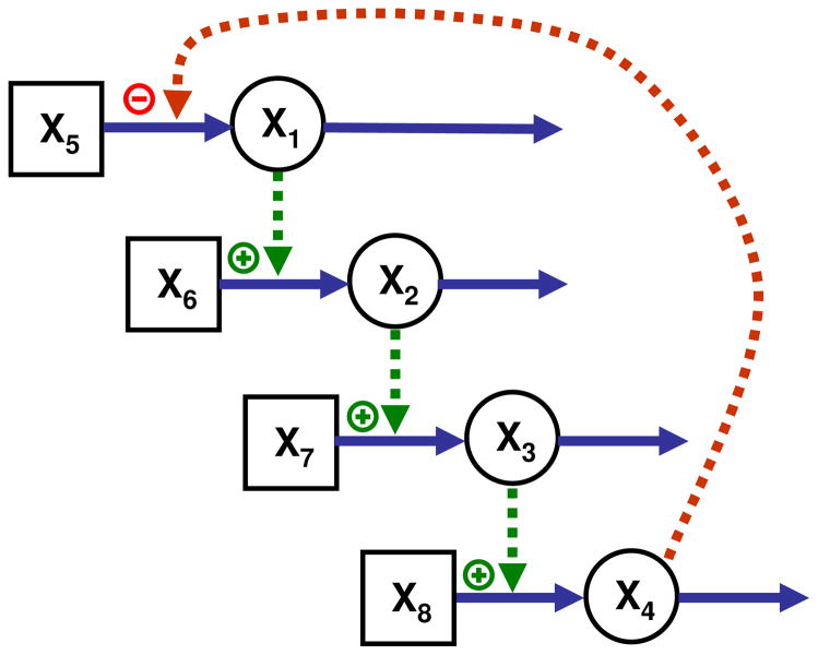
It is useful to demonstrate the theoretical results with simple didactic examples. The first representative case is a cascaded system (Fig. 1), where the numbers of precursors and state variables are the same (n = m = 4) and the system has a unique solution. The cascade could describe the expression of a formerly inactive gene X₅, which becomes activated (X₁) and is subsequently transcribed; X₆ could model nucleotides that are assembled into mRNA (X₂); X₇ could represent amino acids, which are assembled into an enzyme (X₃), which subsequently catalyzes the conversion of a metabolic substrate X₈ into a product X₄. The final product could directly or indirectly repress the expression of the gene. The generic S-system representation of the model is

Figure 1.

A cascaded system with as many dependent (circles) as independent (squares) variables. The cascade could represent, from top to bottom, gene expression, transcription into mRNA, translation into protein, and a metabolic process catalyzed by enzyme X₃.

$$\begin{array}{l}{\stackrel{.}{X}}_1={\alpha }_1{X}_4^{g_{14}}{X}_5^{g_{15}}-{\beta }_1{X}_1^{h_{11}}\\ {\stackrel{.}{X}}_2={\alpha }_2{X}_1^{g_{21}}{X}_6^{g_{26}}-{\beta }_2{X}_2^{h_{22}}\\ {\stackrel{.}{X}}_3={\alpha }_3{X}_2^{g_{32}}{X}_7^{g_{37}}-{\beta }_3{X}_3^{h_{33}}\\ {\stackrel{.}{X}}_4={\alpha }_4{X}_3^{g_{43}}{X}_8^{g_{48}}-{\beta }_4{X}_4^{h_{44}}\end{array}$$ (11)

Without loss of generality in this and the later illustration examples, all rate constants α_i and β_i are arbitrarily set to 1 and the independent variables are initially defined as 1.2. By this definition we know that y′_D = y_D because b = 0. The values of the kinetic order parameters in this and other systems are given in Table 1.

Table 1.

Numerical Values of Kinetic Parameters for All Illustration Examples^*

Cascade 1		Linear Pathway		Cascade 2		Branched Pathway
Fig. 1		Fig. 2		Fig. 4		Fig. 7
g14	−0.8	g15	0.5	g14	−0.8	α1	1.755	β1	1
g15	0.25	g21	0.2	g15	0.24	α2	1	β2	2
g21	0.4	g24	−0.25	g21	0.4	α3	1	β3	2
g26	0.3	g32	0.8	g26	0.3	α4	1	β4	1
g32	0.5	g36	0.35	g32	0.5	g13	0.05	h11	1
g37	0.3	g43	0.4	g37	0.3	g15	0.75	h16	1
g43	0.1	g47	0.1	g43	0.4	g1,11	0.125	h22	0.5
g48	0.2	h11	0.2	h11	0.2	g21	1	h27	0.5
h11	0.2	h14	−0.25	h22	1	g26	1	h29	0.5
h22	1	h22	0.8	h33	0.8	g32	0.5	h33	0.2
h33	0.4	h26	0.35	h44	0.9	g39	1	h3,10	0.25
h44	0.2	h33	0.4			g42	0.5	h3,11	0.25
		h37	0.1			g47	1	h44	0.5
		h44	0.2					h48	1
		h48	0.25

^*The rate constants for the linear and the two cascaded pathways were set equal to 1.

The second example is a simple linear pathway with feedback and an exogenous demand for product (Fig. 2). This example was chosen in contrast to the cascaded system, because it involves several precursor-product relationships, which constrain the parameters of the corresponding effluxes and influxes. While one may initially wonder what the effects of these constraints may be, we will see that these constraints have no real bearing on the characterization of a set of independent variables that moves the system to the target steady state. The enzymes for the conversions of X₂ into X₃ and X₄ are explicitly modeled, as are the input to the pathway and the demand for X₄, such that n = m = 4. The generic S-system model is

Fig. 2.

Linear pathway with feedback and an exogenous demand for product. The task of moving the system to a new steady state has a unique solution.

$$\begin{array}{l}{\stackrel{.}{X}}_1={\alpha }_1{X}_5^{g_{15}}-{\beta }_1{X}_1^{h_{11}}{X}_4^{h_{14}}\\ {\stackrel{.}{X}}_2={\beta }_1{X}_1^{h_{11}}{X}_4^{h_{14}}-{\beta }_2{X}_2^{h_{22}}{X}_6^{h_{26}}\\ {\stackrel{.}{X}}_3={\beta }_2{X}_2^{h_{22}}{X}_6^{h_{26}}-{\beta }_3{X}_3^{h_{33}}{X}_7^{h_{37}}\\ {\stackrel{.}{X}}_4={\beta }_3{X}_3^{h_{33}}{X}_7^{h_{37}}-{\beta }_4{X}_4^{h_{44}}{X}_8^{h_{48}}\end{array}$$ (12)

Again, all rate constants α_i and β_i are arbitrarily set to 1 and the independent variables to 1.2. The values of the kinetic orders are given in Table 1.

For our illustration, we start both systems arbitrarily at (1, 1, 1, 1) and let them reach their nominal steady states. While at the steady state, the environmental demand changes at time t = 60 or t = 150, respectively, and we assume that all variables in the cascade and the linear pathway must move to a new target value of 2. Because n = m = 4, the solutions are in both cases unique. They are given as ${\mathbf{X}}_I={[\begin{array}{llll}16.0\hfill & 4.0\hfill & 0.7937\hfill & 1.4142\hfill \end{array}]}^{\text{T}}$ and ${\mathbf{X}}_I={[\begin{array}{llll}0.933\hfill & 0.1857\hfill & 0.0442\hfill & 0.5\hfill \end{array}]}^{\text{T}}$, respectively. Numerical simulation demonstrates that the systems indeed respond by moving to the desired target states (Fig. 3). The vectors X_I in the inverse solutions do not convey anything about the transients.

Fig. 3.

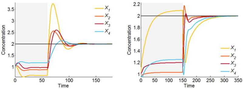
Resetting the independent variables according to the computed unique solutions moves the cascaded (left) and linear (right) pathway systems to the desired target (2, 2, 2, 2). During the initial phase (shaded light grey), the systems move from their arbitrary initial values (1, 1, 1, 1) to their nominal steady states. At time t = 60 or t = 150, respectively, the environment changes, requiring all variables to reach the target value 2.

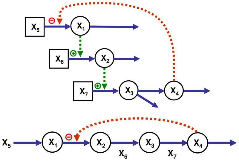
The third and fourth introductory examples are cascaded and linear pathways with fewer independent than dependent variables (Fig. 4). S-systems models were constructed according to well-documented guidelines, and the values of the kinetic orders for the cascaded system were defined as presented in Table 1. The target values were defined as 3. It could seem that theses scenarios are rather unrealistic, but they do occur in cases like the ones shown here as well as in cases of strongly connected pathways where not all genes or enzymes are accessible to manipulations. If it is infeasible or impossible to alter some of the independent variables, m is in effect decreased and may become lower than n.

Figure 4.

Over-determined cascaded and linear pathway systems with n = 4, m = 3. In the example of a linear pathway, the reaction between X₁ and X₂ may not be accessible to alterations.

This “unsolvable” situation may be addressed in different ways. First, instead of searching for an exact solution, one may solve the corresponding regression problem (see Eq. 8) and find a set of independent variables that moves the system to a steady state that is as close as possible to the target state (Fig. 5). In the numerical example here, the solution vector is ${\mathbf{X}}_I={[\begin{array}{lll}17.7905\hfill & 9\hfill & 5.4885\hfill \end{array}]}^{\text{T}}$, and we see that X₃ and X₄ are not quite on target.

Figure 5.

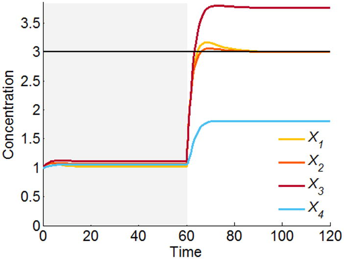
Least squares solution for the over-determined cascaded system in Figure 4.

As a variation on this theme, closeness to the target state may be defined differently for each dependent variable, through the use of appropriate weights. This strategy allows for the option that some “important” dependent variables can be selected to come as closely as possible to their target values, while others are possibly not. Finally, one may ignore some of the dependent variables, whose specific values are not considered as important as those of other variables, and restrict the optimization to a subset of important dependent variables, thereby in effect reducing n. Examples for less important variables might be intermediates in linear pathways,

To be specific, suppose it is most important that variable X₄ of the cascaded pathway attain the target value, while other variables are of secondary importance. The original task can be written as

$${\mathbf{y}}_D=\mathbf{L}{\mathbf{y}}_I\text{where}{y}_{\text{D}}=\left[\begin{array}{l}{y}_1\hfill \\ y_2\hfill \\ y_3\hfill \\ y_4\hfill \end{array}\right],\mathbf{L}=\left[\begin{array}{lll}{L}_{11}\hfill & L_{12}\hfill & L_{13}\hfill \\ L_{21}\hfill & L_{22}\hfill & L_{23}\hfill \\ L_{31}\hfill & L_{32}\hfill & L_{33}\hfill \\ L_{41}\hfill & L_{42}\hfill & L_{43}\hfill \end{array}\right],\text{and}{y}_{\text{I}}=\left[\begin{array}{l}{y}_5\hfill \\ y_6\hfill \\ y_7\hfill \end{array}\right].$$ (13)

To enforce that X₄ moves to the target, presumably at the cost of other variables, we separate the equation for X₄ in Eq. (13) from the rest, which yields

$$y_4=[\begin{array}{lll}{\text{L}}_{41}\hfill & {\text{L}}_{42}\hfill & {\text{L}}_{43}\hfill \end{array}]\left[\begin{array}{l}{y}_5\hfill \\ y_6\hfill \\ y_7\hfill \end{array}\right].$$ (14)

Using the notation ${\mathbf{L}}_{123}=\left[\begin{array}{lll}{\text{L}}_{11}\hfill & {\text{L}}_{12}\hfill & {\text{L}}_{13}\hfill \\ {\text{L}}_{21}\hfill & {\text{L}}_{22}\hfill & {\text{L}}_{23}\hfill \\ {\text{L}}_{31}\hfill & {\text{L}}_{32}\hfill & {\text{L}}_{33}\hfill \end{array}\right]$ and ${\mathbf{L}}_4=[\begin{array}{lll}{\text{L}}_{41}\hfill & {\text{L}}_{42}\hfill & {\text{L}}_{43}\hfill \end{array}]$, the particular solution of

y_I based on this separated equation is now given as

$${\mathbf{y}}_I={\mathbf{y}}_{I\_PS}+{\mathbf{B}}_4·\mathbf{\lambda },$$ (15)

where

$${\mathbf{y}}_{I\_PS}={\mathbf{L}}_4^{+}{y}_4,$$ (16)

B₄ is a 3×2 matrix where each column is a basis vector of the null space of L, and λ is any real-valued 2-dimensional vector. Having enforced that the fourth variable will reach the target value, we still have options for the remaining independent variables. Namely, the equation

$$\begin{array}{l}{[\begin{array}{lll}{y}_1\hfill & y_2\hfill & y_3\hfill \end{array}]}^T={\mathbf{L}}_{123}{\mathbf{y}}_I\\ ={\mathbf{L}}_{123}({\mathbf{y}}_{I\_PS}+{\mathbf{B}}_4·\mathbf{\lambda })\end{array}$$ (17)

allows us to define criteria such as a least-squares error for the remaining variables, which correspond to different choices for λ. For instance, we can use the pseudo-inverse to define

$$\mathbf{\lambda }={({\mathbf{L}}_{123}·{\mathbf{B}}_4)}^{+}\left({[\begin{array}{lll}{y}_1\hfill & y_2\hfill & y_3\hfill \end{array}]}^T-{\mathbf{L}}_{123}·{\mathbf{y}}_{I\_PS}\right),$$ (18)

which yields the solution as

$${\mathbf{y}}_I={\mathbf{y}}_{I\_PS}+{\mathbf{B}}_4·{({\mathbf{L}}_{123}·{\mathbf{B}}_4)}^{+}\left({[\begin{array}{lll}{y}_1\hfill & y_2\hfill & y_3\hfill \end{array}]}^T-{\mathbf{L}}_{123}·{\mathbf{y}}_{I\_PS}\right).$$ (19)

The result of this operation is shown in Fig. 6. In comparison with Fig. 5, X₄ now reaches the target value 3 exactly, while the remaining variables approach the value 3 only approximately. In particular, the improvement in X₄ is “paid for” with an inferior performance of X₃. The solution vector of independent variables in this case is ${\mathbf{X}}_I={[\begin{array}{lll}97.2759\hfill & 9.0\hfill & 116.8222\hfill \end{array}]}^{\text{T}}$. If X₃ is most important in the same system, the solution vector is ${\mathbf{X}}_I={[\begin{array}{lll}12.7188\hfill & 9.0\hfill & 3.0\hfill \end{array}]}^{\text{T}}$ and X₄ overshoots the target (plot not shown).

Figure 6.

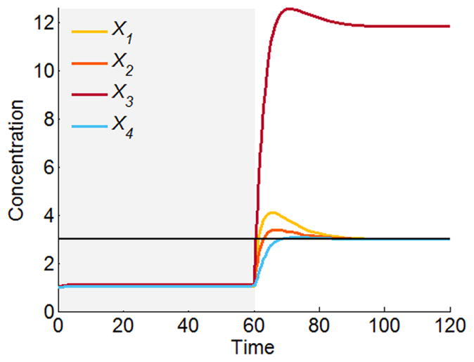
Solution for the over-determined cascaded system in Figure 4, where X₄ is forced to reach the target state 3.

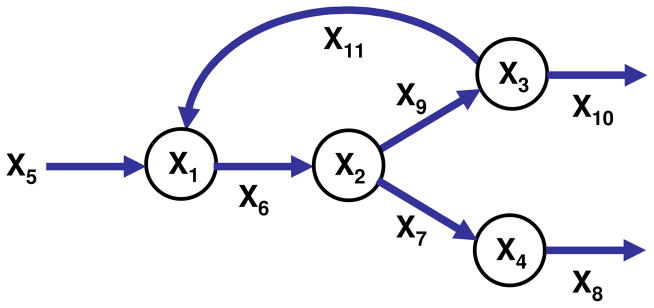
The most pertinent case is n < m. A representative example is the pathway shown in Fig. 7, which has four dependent and seven independent variables. The S-system was constructed according to usual guidelines (see Table 1 for parameter values), and as before, we set all independent variables arbitrarily set to 1.2 and solved the system from (1, 1, 1, 1) to its normal steady state. Subsequently, we assumed that the environmental demand changed by requiring all target values for the dependent variables to assume the value of 2.

Figure 7.

Branched pathway with a substrate cycle. The system contains four dependent variables (circles) and seven independent variables, which model the system input (X₅) and catalyzing enzymes (X₆, …, X₁₁). The system is representative of the most prevalent situation where n < m.

Because n < m, the solution consists of a space that can be expressed by a particular solution plus a linear span of a basis of the null space of $\mathbf{L}=-{\mathbf{A}}_D^{-1}{\mathbf{A}}_I$. The particular solution is computed as

$${\mathbf{y}}_D=\mathbf{L}{\mathbf{y}}_I$$ (20)

$${\mathbf{y}}_{I\_PS}={\mathbf{L}}^{+}{\mathbf{y}}_D$$ (21)

and any feasible solution can be characterized by the particular solution plus an arbitrary vector in the null space of L:

$${\mathbf{y}}_I=\mathbf{B}·\mathbf{\lambda }+{\mathbf{y}}_{I\_PS}.$$ (22)

where λ may be any 3-dimensional real-valued vector and B is a matrix in which each column is a basis vector of the null space of L.

Choosing any y_I inside this solution space is guaranteed to lead the system to the target steady state. Two examples of admissible solutions in Cartesian space are ${\mathbf{X}}_I={[\begin{array}{lllllll}1.9363\hfill & 1.4646\hfill & 0.7293\hfill & 0.7293\hfill & 1.4705\hfill & 0.7755\hfill & 0.8658\hfill \end{array}]}^{\text{T}}$ and ${\mathbf{X}}_I={[\begin{array}{lllllll}4.3355\hfill & 2.8505\hfill & 2.1973\hfill & 2.1973\hfill & 1.8490\hfill & 1.1861\hfill & 1.4149\hfill \end{array}]}^{\text{T}}$. The former of these solutions is the least-squares solution, while the latter is the least-squares solution plus the first basis vector of the null space. These and other solutions within the admissible space move the system to the target steady state of (2, 2, 2, 2) as expected, but the transient behaviors of these systems are different, and it is not a priori clear how to manipulate them.

Interestingly, it is possible to alter any solution to some degree in a targeted fashion by controlling the basis vectors of the three-dimensional null space of L. In the given numerical case, the basis vectors are

$$\begin{array}{l}{\mathbf{B}}_1={[\begin{array}{lllllll}0.403\hfill & 0.333\hfill & 0.5514\hfill & 0.5514\hfill & 0.1145\hfill & 0.2124\hfill & 0.2456\hfill \end{array}]}^{\text{T}},\\ {\mathbf{B}}_2={[\begin{array}{lllllll}0.0226\hfill & 0.0091\hfill & -0.1991\hfill & -0.1991\hfill & 0.2173\hfill & 0.9322\hfill & -0.063\hfill \end{array}]}^{\text{T}},\\ {\mathbf{B}}_3={[\begin{array}{lllllll}-0.1285\hfill & 0.0201\hfill & -0.1776\hfill & -0.1776\hfill & 0.2178\hfill & -0.0607\hfill & 0.9321\hfill \end{array}]}^{\text{T}}.\end{array}$$ (23)

These basis vectors can be computed directly in Matlab with the Null command, which applies singular value decomposition to obtain an orthogonal basis set. Different effects are observed when any of these basis vectors is altered. For instance, increasing B₁ by a positive factor causes all responses to speed up (Fig. 8), while increasing B₂ or B₃ causes X₁, X₂ and X₃ to accelerate but X₄ to slow down (data not shown). Thus, the transient behavior can be controlled to some degree through the basis vectors. However, the effects of such manipulations are difficult to predict, and it is more straightforward to use direct optimization methods as we will discuss them next.

Figure 8.

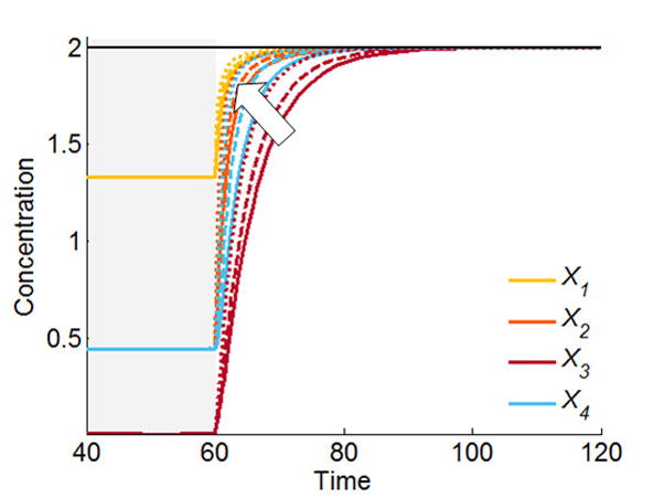
Manipulation of the basis vectors permits modest changes in transient speed. Here, increasing B₁ causes all transients to accelerate (arrow). Solid lines: no acceleration; dashed lines: acceleration by increasing B₁ twofold; dotted lines: acceleration by increasing B₁ fourfold.

Optimal Operating Strategies

The computation of the pseudo-inverse in the steady-state equations of the S-system, along with the characterization of the null space, results in the space of all possible solutions. Within this space, any computed resetting of the independent variables leads to a desired steady state in terms of the dependent variables. While it is mathematically and practically satisfying to have a concise representation of this solution space, one will wonder whether some admissible solutions within this space are “better” than others. Clearly, the answer requires optimization, which, interestingly, does not need an explicit characterization of the solution space per se. The optimization does require an objective function, which is to be selected according to the chosen criteria of functional effectiveness.

Operating principles have not yet been analyzed often enough to permit a listing of “typical” criteria of functional effectiveness, and judging by the exploration of design principles, one might expect them to change from one application to another. Among likely, generic criteria one will often establish similar metrics as for design principles, which often include local stability, modest gains and sensitivities, and tolerance of the steady state to perturbations. Also as in the case of design principles, one might prefer fast response times and bounded transients. Another typical criterion in superior designs is a minimal accumulation of intermediates. Here, this criterion is automatically satisfied when a complete target profile of steady-state values is mandated, but if no target values for intermediates are specified, it may indeed serve as a criterion.

In addition to these criteria gleaned from design principle analysis, operating strategies are distinguishable in other respects. In the work presented here, we focus primarily on two aspects that appear to be particularly pertinent: the collective deviation of independent variables from their nominal levels, and the number of independent variables that are to be changed. These criteria are important to a cell, because they are directly related to the effort that has to be expended in terms of gene expression and the dynamics of RNAs and proteins [40], and to the degree of possible side effects from such changes. Secondarily, we will look into the profiles of transients between steady states. One could presumably study a variety of additional criteria, such as a favorable dynamic sensitivity profile [41; 42].

To formalize the deviation from normal operation, we introduce a vector d that represents the change in the vector of independent variables such that the system reaches the target steady state y∼_D, which is assumed to be known. With these definitions, we can formulate the target state as

$${\stackrel{\sim }{\mathbf{y}}}_D={\mathbf{A}}_D^{-1}\mathbf{b}-{\mathbf{A}}_D^{-1}{\mathbf{A}}_I({\mathbf{y}}_I+\mathbf{d}),$$ (24)

and this expression can be rearranged as a linear constraint on d. Namely, we can write

$${\mathbf{A}}_D^{-1}{\mathbf{A}}_I\mathbf{d}={\mathbf{A}}_D^{-1}(\mathbf{b}-{\mathbf{A}}_I{\mathbf{y}}_I)-{\stackrel{\sim }{\mathbf{y}}}_D.$$ (25)

Now let

$$z_i=\{\begin{array}{ll}1\hfill & \text{if}\text{the}\text{catalytic}\text{step}\text{coded}\text{by}{d}_i\text{is}\text{induced}\text{to}\text{reach}\text{the}\text{steady}\text{state}\hfill \\ 0\hfill & \text{otherwise}\hfill \end{array}.$$ (26)

If all z_i are set to 1, the optimization task allows every independent variable to change as long as the linear constraints are satisfied, but the identification of specific solutions still depends on the dimension and rank of ${\mathbf{A}}_D^{-1}{\mathbf{A}}_I$ as well as the chosen criteria of functional effectiveness.

One of the most commonly used criteria for finding a particular solution is the total squared error E, which in this case can be written as

$$E={\Vert {\mathbf{A}}_D^{-1}(\mathbf{b}-{\mathbf{A}}_I{\mathbf{y}}_I)-{\stackrel{\sim }{\mathbf{y}}}_D-{\mathbf{A}}_D^{-1}{\mathbf{A}}_I\mathbf{d}\Vert }^2,$$ (27)

where ||•||² is the 2-norm. The solution d̂ with the lowest E corresponds to an optimal operating strategy where the first criterion, i.e., the collective deviation in independent variables from their nominal values, is minimized.

The second criterion requires finding a minimum set of independent variables whose alteration is necessary for reaching the target steady state. This task is equivalent to solving the following Mixed Integer Linear Programming (MILP) problem:

$$\begin{array}{l}min\sum _{i=1}^m{z}_i\text{subject}\text{to}\\ {\mathbf{A}}_D^{-1}{\mathbf{A}}_I\mathbf{d}={\mathbf{A}}_D^{-1}(\mathbf{b}-{\mathbf{A}}_I{\mathbf{y}}_I)-{\stackrel{\sim }{\mathbf{y}}}_D\\ d_i\ge 0\\ d_i\le z_{i}D(\text{D}\text{is}\text{an}\text{arbitrarily}\text{large}\text{positive}\text{number})\\ z_i:0/1\\ \forall i=1,\dots ,m\end{array}$$ (28)

The CPLEX solver in AMPL can be used to solve this type of MILP.

Similar to optimization tasks in the field of biotechnology, where the typical objective is the maximization of a metabolite pool or flux, it is here also possible to account for constraints on concentrations and fluxes [43; 44; 45; 46; 47] as well as more complex limitations such as metabolic burden [9] or the feasibility of parameter regions that correspond to admissible physiological states [28]. In particular, the metabolic burden, which is associated with the total mass of all protein (cf. discussion in [9]), can be an important issue of cellular protein economy because it was shown for the case of recombinant bacteria that the growth rate decreased monotonically with increasing numbers of introduced plasmid copies (e.g., [48; 49; 50]).

Moreover, one should expect that it is easier to up- or down-regulate some genes or enzyme activities than others. In fact, it might not be practically feasible to change some enzyme activities at all. If so, the corresponding independent variables in the model are off limits in the selection of any viable operating strategies. Other processes might be accessible to manipulations but limited in the degree of alteration. We will discuss some of these concepts in the following Case Study.

Case Study

As a specific case study, we consider the response of yeast cells to heat stress. The first indications of such a response are observable within minutes of the initiation of heat stress: transcription factors are mobilized and translocated [51], and numerous genes respond with strong changes in expression [52; 53; 54]. At the proteomic level, heat shock proteins emerge in high numbers [55; 56; 57]. At the metabolic level, a significantly altered profile of sphingolipids guides the expression of some key genes [58], and, most important for the following illustration, the protective disaccharide trehalose is produced in huge amounts [40; 59].

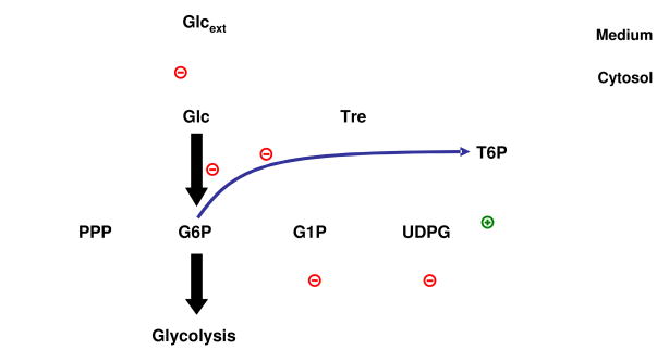
Several modeling studies have investigated the dynamics of trehalose upon heat shock in recent years [14; 26; 28; 29; 40; 60; 61], which allows us to keep the discussion of background information to a minimum. In a nutshell, material is siphoned off glycolysis at the level of glucose 6-phosphate and channeled toward the production of glucose 1-phosphate, UDPG, glycogen, trehalose 6-phospate and trehalose, with trehalose accumulating in large quantities. The enzyme trehalase splits trehalose into two glucose molecules and thereby completes the trehalose cycle (see Fig. 9). Because the present study is focused on methodological advances rather than new biological insights, we take the S-system model of the trehalose cycle in [14] at face value and analyze alternative operating strategies.

Figure 9.

The S-system equations describing the system were taken directly from [14]. They are

$$\begin{array}{l}\text{Glucose}:{\stackrel{.}{X}}_1=31.912X_0^{0.968}{X}_2^{-0.194}{X}_7^{0.00968}{X}_8^{0.968}{X}_{19}^{0.0323}-89.935X_1^{0.75}{X}_6^{-0.4}{X}_9\\ \text{G6P}:{\stackrel{.}{X}}_2=142.72X_1^{0.517}{X}_2^{-0.179}{X}_3^{0.183}{X}_6^{-0.276}{X}_9^{0.689}-X_{12r}^{0.311}-30.120X_1^{-0.00333}{X}_2^{0.575}{X}_3^{-0.17}{X}_4^{0.00333}{X}_{10}^{0.5111}{X}_{11}^{0.0667}{X}_{12f}^{0.411}{X}_{17}^{0.0111}\\ \text{G1P}:{\stackrel{.}{X}}_3=7.8819X_2^{0.394}{X}_3^{-0.392}{X}_4^{-0.010}{X}_5^{0.0128}{X}_{12f}^{0.949}{X}_{15r}^{0.0513}-76.434X_2^{-0.412}{X}_3^{0.593}{X}_{12r}^{0.718}{X}_{13}^{0.180}{X}_{15f}^{0.103}\\ \text{UDPG}:{\stackrel{.}{X}}_4=11.070X_3^{0.5}{X}_{13}-3.4556X_1^{\mathrm{-0.0429}}{X}_2^{0.214}{X}_4^{0.386}{X}_{14}^{0.857}{X}_{17}^{0.143}\\ \text{Glycogen}:{\stackrel{.}{X}}_5=11.060X_2^{0.040}{X}_3^{0.320}{X}_4^{0.160}{X}_{14}^{0.600}{X}_{15f}^{0.400}-4.9290X_2^{-0.04}{X}_4^{-0.04}{X}_5^{0.25}{X}_{15r}^{0.200}{X}_{16}^{0.800}\\ \text{T}6\text{P}:{\stackrel{.}{X}}_6=0.19424X_1^{-0.300}{X}_2^{0.300}{X}_4^{0.300}{X}_{17}-1.0939X_6^{0.200}{X}_{18}\\ \text{Trehalose}:{\stackrel{.}{X}}_7=1.0939X_6^{0.200}{X}_{18}-1.2288X_7^{0.300}{X}_{19}\end{array}$$ (29)

Of primary interest here is the response of yeast to heat stress, which affects most of the reactions steps in the pathway. According to literature studies (cited in [14]), the alterations among the dependent and independent variables under heat stress are distinctly different, with some variables and steps changing substantially and others not as much or not at all (Tables 2 and 3).

Table 2.

Dependent variables of the canonical model (Eq. 29) of the trehalose cycle. Steady-state values under optimal temperature conditions were collected from the literature [14]; heat-stress values (scaled by optimal steady-state values) computed with the S-system model upon changes in independent variables as shown in Table 4

Metabolite	Variable Name	Steady-State Concentration [mM] under Optimal Temperature Conditions (from the Literature)	Computed Fold Change in Steady-State Concentration during Heat Stress (Scaled by Normal Steady State)
Glucose	X1	0.03	1.46
Glucose 6-Phosphate	X2	1	5.54
Glucose 1-Phosphate	X3	0.1	3.99
Uridine Diphosphate Glucose	X4	0.7	2.69
Glycogen	X5	1	55.8
Trehalose 6-Phosphate	X6	0.02	4.28
Trehalose	X7	0.05	103

Table 3.

Different implementations of computed heat stress responses, which all lead to exactly the same target steady state

Catalytic or Transport Step	Variable Name	Nominal*	Least Squares	Minimum Set	Least Squares (X8, X10, $V_5^{+}$ and $V_7^{+}$ fixed)	Minimum Set (X8, X10, $V_5^{+}$ and $V_7^{+}$ fixed)
Glucose transport	X8	8	2.0096	4.6155	8 (fixed)	8 (fixed)
Hexokinase/Glucokinase	X9	8	1.9440	4.4334	8	8
Phosphofructokinase	X10	1	0.3577	1	1 (fixed)	1 (fixed)
G6P dehydrogenase	X11	6	0.8745	1	6.2371	1.6377
Phosphoglucomutase	X12	16	0.8435	1.1046	15.5916	38.0406
UDPG pyrophosphorylase	X13	16	1.1110	1.5932	14.9673	149.5541
Glycogen synthase	X14	16	1.0616	1.4620	14.8016	217.1534
Glycogen phosphorylase	X15	50	1.0512	1	56.1937	1
Glycogen use	X16	16	0.7965	1	15.5396	42.5464
α, α-T6P synthase	X17	12	1.0942	2	12	12
α, α-T6P phosphatase	X18	18	1.6413	3	18	18
Trehalase	X19	6	0.5471	1	6	6

^*Heat-induced fold-increase in activity used in the model (Eq. 29)

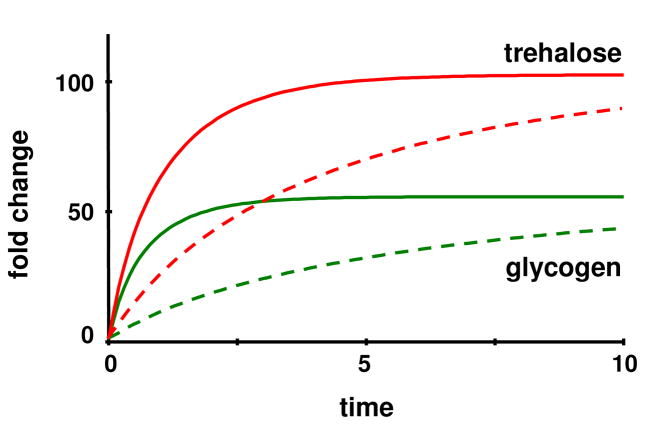
In this case, n = 7 and m = 12, which indicates quite a bit of flexibility among different solutions. Application of the pseudo-inverse method reveals the space of all admissible solutions; an example of a possible solution is ${\mathbf{X}}_I={[\begin{array}{llllllllllll}5.4169\hfill & 5.2877\hfill & 0.9723\hfill & 2.3770\hfill & 2.3004\hfill & 3.0197\hfill & 2.8855\hfill & 2.8574\hfill & 2.1650\hfill & 2.9739\hfill & 4.4620\hfill & 1.4873\hfill \end{array}]}^{\text{T}}$. X_I is computed using the pseudo-inverse of L and the original basis of the null space of L, which was obtained through singular value decomposition in MATLAB, and $\mathbf{\lambda }={[\begin{array}{lllll}1\hfill & 1\hfill & 1\hfill & 1\hfill & 1\hfill \end{array}]}^{\text{T}}$. As to be expected, this vector of independent variables moves the system to the target steady state. However, the solution is much slower than the observed solution (Fig. 10).

Figure 10.

A possible solution within the space characterized by the pseudo-inverse method (dashed), in comparison with the nominal solution discussed in [14]. While both solutions eventually reach the same steady state, the transient of the solution computed here is comparatively slow (see text for details).

The solution space obtained with the pseudo-inverse method is 5-dimensional, and a basis is

$$\begin{array}{l}{\mathbf{B}}_1={[\begin{array}{llllllllllll}0.1635\hfill & 0.1582\hfill & 0.2144\hfill & -0.1562\hfill & 0.0986\hfill & -0.1328\hfill & -0.1543\hfill & 0.9026\hfill & 0.1099\hfill & -0.0034\hfill & -0.0034\hfill & -0.0034\hfill \end{array}]}^{\text{T}}\\ {\mathbf{B}}_2={[\begin{array}{llllllllllll}-0.2260\hfill & -0.2188\hfill & -0.3985\hfill & 0.2716\hfill & 0.3480\hfill & 0.3708\hfill & 0.4330\hfill & 0.2639\hfill & 0.3907\hfill & -0.0017\hfill & -0.0017\hfill & -0.0017\hfill \end{array}]}^{\text{T}}\\ {\mathbf{B}}_3={[\begin{array}{llllllllllll}-0.2260\hfill & -0.2087\hfill & -0.1967\hfill & -0.7547\hfill & 0.0363\hfill & 0.0466\hfill & 0.0021\hfill & 0.0002\hfill & 0.0016\hfill & 0.3128\hfill & 0.3128\hfill & 0.3128\hfill \end{array}]}^{\text{T}}\\ {\mathbf{B}}_4={[\begin{array}{llllllllllll}0.3576\hfill & 0.3568\hfill & 0.4235\hfill & 0.1207\hfill & 0.1771\hfill & 0.2723\hfill & 0.2627\hfill & -0.1569\hfill & 0.1578\hfill & 0.3301\hfill & 0.3301\hfill & 0.3301\hfill \end{array}]}^{\text{T}}\\ {\mathbf{B}}_5={[\begin{array}{llllllllllll}-0.1451\hfill & -0.1291\hfill & -0.2276\hfill & 0.5556\hfill & -0.1360\hfill & -0.2193\hfill & -0.3147\hfill & 0.1558\hfill & -0.1971\hfill & 0.3527\hfill & 0.3527\hfill & 0.3527\hfill \end{array}]}^{\text{T}}\end{array}$$

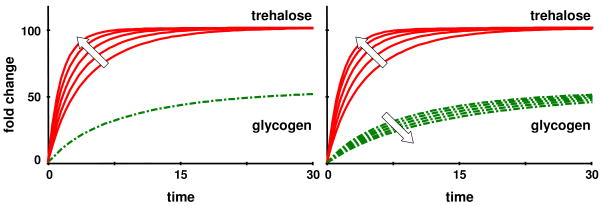
As in the illustrative example of a branched pathway, it is to some degree possible to affect the transient speed by manipulating the basis vectors. Tuning B₁ or B₂ causes the glycogen concentration to speed up but has almost no effect on trehalose or the other variables. Increasing B₃ accelerates trehalose and no other variables, increasing B₄ speeds up both trehalose and glycogen, while increasing B₅ speeds up trehalose but slows down glycogen production (Fig. 11).

Figure 11.

The solutions obtained with the pseudo-inverse method can be manipulated by modifying the basis vectors. In the left panel, basis vector B₃ was multiplied with factors 1, …, 5 (in direction of the arrow); this action did not affect the glycogen profile. In the right panel, basis vector B₅ was multiplied with factors 1, …, 5, in direction of the arrows. All solutions eventually reach the same target steady state.

In contrast to exploring the entire solution space, the direct optimization method allows us to select criteria of functional effectiveness a priori and to optimize the solution toward these criteria under the constraint that the target steady state is reached. As the first example, suppose the overriding criterion is to alter the independent variables as little as possible in magnitude. Least-squares optimization toward this criterion yields a solution that not only reaches the target steady state but also exhibits only modest variations in enzyme activities (Table 3; column 4).

As a second example, we mandate to keep the number of altered independent variables to a minimum. MILP optimization reveals that this minimum number is 7, and the steady state is reached upon quite strong alterations in this minimum set (Table 3; column 5).

There are unlimited combinations on this theme, depending on the choice of criteria of functional effectiveness. For instance, we may consider a more complex scenario, which accommodates the following criteria. First, suppose that the phosphofructokinase step (X₁₀) cannot be altered. This supposition was motivated by actual observations in yeast (cf. [26]), and rationale for this restriction was presented based on different types of analyses [28; 29]. The restriction is easy to implement by fixing X₁₀ = 1. Secondly, 20 transporters are involved in glucose uptake and fine tuned for different glucose concentrations in the medium, which may mean that the glucose transport step probably cannot be altered effectively from what is observed. Thus, we enforce X₈ = 8, which corresponds to the observed level. Third, the rates of glycogen and trehalose production ( $V_5^{+}$ and $V_7^{+}$) should be sufficiently large to achieve a timely response to elevated temperatures, which we implement by setting these flux rates to those actually observed and not permitting them to be altered. If subscript e indicates the nominal steady-state values under heat stress condition (as discussed in [14]), we obtain

$$\begin{array}{l}{V}_5^{+}=V_{5e}^{+}\\ \Rightarrow ln{\alpha }_5+0.04y_{2e}+0.32y_{3e}+0.16y_{4e}+0.6y_{14}+0.4y_{15}=ln{\alpha }_5+0.04y_{2e}+0.32y_{3e}+0.16y_{4e}+0.6y_{14e}+0.4y_{15e}\\ \Rightarrow 0.6y_{14}+0.4y_{15}=0.6y_{14e}+0.4y_{15e}\\ V_7^{+}=V_{7e}^{+}\\ \Rightarrow ln{\alpha }_7+0.2y_{6e}+y_{18}=ln{\alpha }_7+y_{6e}+y_{18e}\\ \Rightarrow y_{18}=y_{18e}\end{array}$$

These conditions impose further constraints on the system and are easily formulated in the MILP. The size of the solution space (number of free variables minus the number of linearly independent equality constraints) is now drastically reduced from 5 to 1. Within the constrained system, we can again identify the minimal set or least squares solution (Table 3, Columns 6 and 7) or could use some other criterion of function effectiveness.

Both results are interesting. First, the constrained least-squares solution turns out to be very similar to the nominal solution, which indicates a similar strategy as in the case of the diauxic shift (see introduction and [25]). Second, the minimum-set solution shows drastically different values than the nominal solution and identifies glycogen phosphorylase as the most dispensable reaction step. In an entirely different study [62], this same step was also identified as only modestly relevant for the trehalose response. The question of which strategy is superior depends on the criteria of functional effectiveness. One might say that the least-squares solution should be the preferred means of operation because all variables remain as close to their normal operating points as possible and the strategy produces glycogen faster. Yet, if the cost of gene expression and the production of transcription factors and mRNAs is a major concern, then the minimum-set solution might be superior because its sum of independent variables is smaller. In short, the superiority is context-dependent rather than universal.

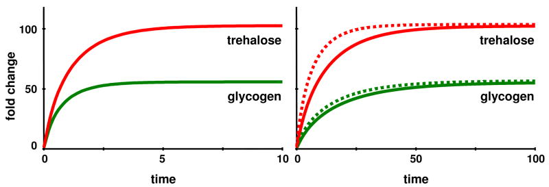
Table 3 seems to indicate that much “cheaper” solutions than the nominal solution can be found, which raises the question of why the nominal solution employs alterations in independent variables that are so much more dramatic than the least squares or minimum set solutions. At least one answer can be found in the response time: although all solutions reach exactly the same steady state, the nominal solution is more than ten times faster than the least squares and minimum-set solutions (Figure 12; note different time scales).

Figure 12.

All solutions eventually reach the exact same steady state and the transients have similar shapes, but the timing is quite different. While glycogen and trehalose in the nominal solution come close to their steady state values within about 5 time minutes (left panel), reaching the same levels takes ten or more times as long in the least-squares (right panel; solid lines) and minimum-set (right panel; dotted lines) solutions (note different time scales). Other variables respond on a time scale that is more similar to the nominal solution (not shown).

The issue of drastically different transient speeds begs the question of whether and how the least-squares and minimum-set solutions could be accelerated. The most direct way of accomplishing acceleration arises if every flux contains its own independent variable. For instance, if every flux is governed by an enzyme which enters the flux with a kinetic order of 1, then multiplication by the same factor ϕ > 1 will speed up the dynamics of the entire system by ϕ. This advance does not come for free though, because the cost of the solution with respect to the chosen criterion increases and the result may no longer be optimal. For instance, the metabolic burden, which roughly corresponds to the sum of independent variables, increases ϕ -fold. An increased metabolic burden can be a disadvantage because it puts additional stress on the cell due to higher levels of transcription and translation [48]. If minimal metabolic burden is indeed a pertinent criterion of functional effectiveness, the totality of changes in independent variables should be kept as small as possible.

If the independent variables have different kinetic orders or appear in several equations, a systemic speed-up may still be possible. Specifically, one has to solve the equations

$$\begin{array}{l}\prod _{j=n+1}^{n+m}{\stackrel{\sim }{X}}_j^{g_{ij}}=\varphi \prod _{j=n+1}^{n+m}{X}_j^{g_{ij}}\\ \prod _{j=n+1}^{n+m}{\stackrel{\sim }{X}}_j^{h_{ij}}=\varphi \prod _{j=n+1}^{n+m}{X}_j^{h_{ij}}\end{array}$$

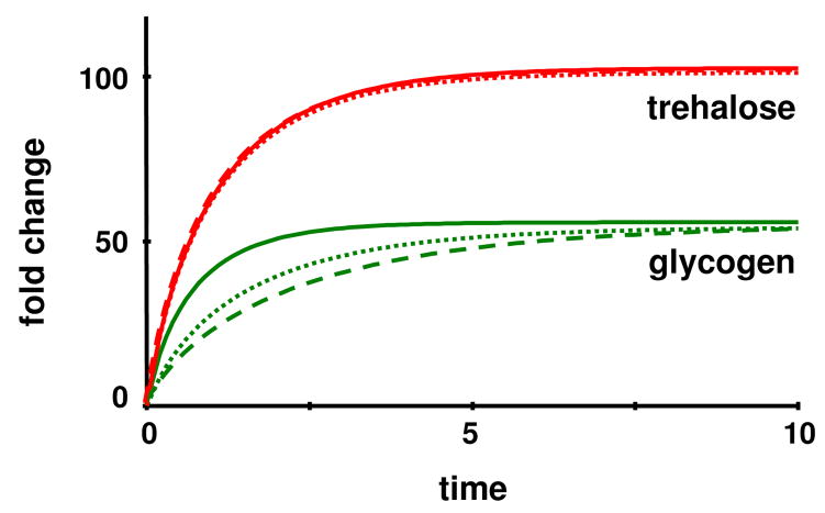
for all i = 1, …, n. In the trehalose case, these conditions result in a set of 14 linear equations with 12 unknowns, which has no algebraic solution. Nevertheless, one can obtain a solution in a least-squares sense, which indeed leads to an acceleration of the transients and approximately reaches the target steady state. The required changes in independent variables are presented in Table 4, where ϕ_LS = 11.19 and ϕ_MS = 6.29 are the acceleration factors for the least-squares and the minimum-set solutions, respectively. These factors are computed based on the settling time τ, which here is the amount of time needed for trehalose to reach and stay within 95% of its nominal heat stress value. While the resulting trehalose profiles are essentially the same as in the nominal scenario, the glycogen trends are still slower (Fig. 13). Interestingly, the steps directly associated with the dynamics of trehalose are very similar to the nominal solution, and the glycogen phosphorylase step is again much lower (Table 4).

Table 4.

Accelerated least squares and minimum set solutions for the trehalose cycle

Catalytic or Transport Step	Nominal	Least Squares (accelerated)	Minimum Set (accelerated)
Glucose transport	8	22.4731	28.8238
Hexokinase/Glucokinase	8	21.7616	27.7065
Phosphofructokinase	1	5.2507	7.9468
G6P dehydrogenase	6	1.2416	1
Phosphoglucomutase	16	9.4252	6.8941
UDPG pyrophosphorylase	16	12.4311	9.9536
Glycogen synthase	16	11.8831	9.1365
Glycogen phosphorylase	50	11.7559	6.2449
Glycogen use	16	8.9158	6.2494
α, α-T6P synthase	12	12.2458	12.4968
α, α-T6P phosphatase	18	18.3691	18.7455
Trehalase	6	6.1230	6.2485

Figure 13.

Acceleration of the least squares (dotted lines) and minimum set (dashed lines) solutions in the trehalose example leads to similar solutions as the nominal case (solid lines), but the accelerated solutions reach the target only approximately (although they come very close). The trehalose trend is now essentially indistinguishable from that in the nominal solution, while the rise in glycogen is slower. Time courses of the other variables essentially match those of the nominal case.

Distinctly different solutions to speeding up the transients could possibly be reached in two ways. First, the cell could initiate a fast transient toward a steady state with more extreme values than needed, and in a second phase relax these values toward the true target state. This strategy is expected to incur overshoots before the true target steady state is reached [35]. Second, it is possible to compute settings in independent variables that reach states that are not steady states. These computations require methods of nonlinear control theory, which were demonstrated for S-systems elsewhere [63].

Discussion

Deciphering how nature solves problems has been the dream of scientists for a long time. Consequently, enormous effort has been devoted to shining light on operating procedures n nature, dissecting systems, and identifying and characterizing processes that cells employ to solve specific problems. Given the seemingly unlimited variability and complexity of tasks that need to be addressed, a comprehensive understanding of operating procedures, let alone operating strategies or even operating principles, will not be gained in the foreseeable future. Nonetheless, the overwhelming magnitude of the challenge does not suggest that we give up, but that even small advances might be beneficial on our long journey.

Thanks to high-throughput techniques of molecular biology, the availability of large datasets has grown immensely and will continue to increase. Along with this increase will be a more and more pressing need to find means of interpretation and of comparing similar, yet structurally different solution strategies. Similar to the investigation of design principles, the study of operating principles is expected to lead to the discovery of motifs, which will provide explanations of naturally evolved systems as well as guidance regarding the design of new systems within the field of synthetic biology.

We have shown in this article that a small sub-class of cellular tasks can be addressed quite efficiently with mathematical and computational tools. Namely, we propose methods for investigating the situation where a biological system is forced to move to a new steady state, which we assume to be known. For example, in the heat stress scenario discussed here, the cell must accumulate sufficient amounts of trehalose and possibly glycogen, while internal glucose and trehalose 6-phosphate need to be carefully controlled, because they cause adverse effects in high concentrations [59; 64; 65]. Thus, some pools in a pathway need to be altered substantially, while others must remain more or less at their nominal level. We show here that such tasks can be formulated rigorously in the language of linear algebra and constrained optimization.

The analysis yields two main results. First, it defines the entire solution space of the problem, and second, it allows a direct system optimization toward given criteria of functional effectiveness. The elegance of these solutions is primarily due to the special structure of S-system models, whose steady states are characterized by systems of linear equations. With the exception of Lotka-Volterra [66; 67; 68] and lin-log models [69; 70], whose steady states are also governed by linear equations, it seems very difficult to obtain similarly general results with ad hoc models, such as pathway systems that are represented with Michaelis-Menten rate laws and their generalizations.

Interestingly, Generalized Mass Action (GMA) representations within BST [10; 71], as well as other model structures, may permit numerical solutions under favorable conditions, although these solutions are not as general as in the case of S-systems. Namely, consider the important special case where each flux representation contains at most one independent variable, which enters the flux in a linear fashion, as it is typical for most enzymes. If all parameter values and the target steady state are known, all terms in the steady-state equations either become linear functions of one independent variable, or they do not contain an independent variable at all. Furthermore, outside the independent variables, all other components of each term combine to a single numerical value, so that the entire system of steady-state equations is linear in the independent variables. As in the cases shown here, this system may have a unique solution or be over- or underdetermined, and it can be analyzed in each case with methods of linear algebra and optimization. The condition of linearity with respect to independent variables can actually be further relaxed, for instance, to the requirement that the same independent variable, if it appears in different terms, always has the same kinetic order.

The tasks and solutions proposed here are reminiscent of optimization problems that have been analyzed in the field for two decades [9; 28; 43; 44; 45; 46]. However, the two lines of investigation represent different aspects of targeted alterations in pathways. In the typical optimization tasks in biotechnology or metabolic engineering, a metabolite pool or flux is to be maximized, while other features of the steady state profile are rather irrelevant as long as they remain within general physiological constraints. As a consequence, the task typically has a clearly defined, single optimal solution, although in some cases alternative optima with the same value of the objective function occur, and it is furthermore possible to investigate multi-objective optimization tasks [9; 72]. In the analysis here, the primary requirement is that the system must reach a specified steady-state profile. This task often admits an entire solution space, within which the system must operate. Within this space, questions of superiority of one solution over another with respect to selected criteria can be explored. Functional effectiveness is not usually considered in biotechnological optimization, but in the case analyzed here provides the metric for comparing alternative strategies and declaring one solution superior to another.

An unresolved issue is the definition of criteria for functional effectiveness, which are not necessarily known a priori. Is it advantageous to up-regulate just a few genes substantially, or is it better to up-regulate many genes by a small amount? We do not yet have answers to such questions, but we have taken a first step by asking these questions and by suggesting that it might be advisable to observe how nature solves tasks in order for us to develop ideas for what types of operating strategies might be candidates for optimality. Moreover, the work presented here suggests tools for comparing different solutions with objectivity and for declaring superiority of different alternatives once criteria are established.

References

- 1.Savageau MA. Advanced Book Program. Addison-Wesley Pub. Co; Reading, Mass: 1976. Biochemical systems analysis : a study of function and design in molecular biology. [Google Scholar]
- 2.Savageau MA. A theory of alternative designs for biochemical control systems. Biomed Biochim Acta. 1985;44:875–880. [PubMed] [Google Scholar]
- 3.Alon U. An Introduction to Systems Biology: Design Principles of Biological Circuits. Chapman & Hall/CRC; Boca Raton, FL: 2006. [Google Scholar]
- 4.Barabási A-L, Oltvai ZN. Network biology: understanding the cell’s functional organization. Nature Reviews Genetics. 2004;5:101–113. doi: 10.1038/nrg1272. [DOI] [PubMed] [Google Scholar]
- 5.Lipshtat A, Purushothaman SP, Iyengar R, Ma’ayan A. Functions of bifans in context of multiple regulatory motifs in signaling networks. Biophys J. 2008;94:2566–2579. doi: 10.1529/biophysj.107.116673. [DOI] [PMC free article] [PubMed] [Google Scholar]
- 6.Ma’ayan A, Cecchi GA, Wagner J, Rao AR, Iyengar R, Stolovitzky G. Ordered cyclic motifs contribute to dynamic stability in biological and engineered networks. Proc Natl Acad Sci USA. 2008;105:19235–19249. doi: 10.1073/pnas.0805344105. [DOI] [PMC free article] [PubMed] [Google Scholar]
- 7.Erdős P, Rényi A. On random graphs. Publicationes Mathematicae. 1959;6:290–297. [Google Scholar]
- 8.Savageau MA. Biochemical systems analysis. I. Some mathematical properties of the rate law for the component enzymatic reactions. J Theor Biol. 1969;25:365–369. doi: 10.1016/s0022-5193(69)80026-3. [DOI] [PubMed] [Google Scholar]
- 9.Torres NV, Voit EO. Pathway Analysis and Optimization in Metabolic Engineering. Cambridge University Press; New York: 2002. [Google Scholar]
- 10.Voit EO. A Practical Guide for Biochemists and Molecular Biologists. Cambridge University Press; Cambridge, UK: 2000. Computational Analysis of Biochemical Systems. [Google Scholar]
- 11.Irvine DH. The method of controlled mathematical comparison. In: Voit EO, editor. Canonical Nonlinear Modeling. Van Nostrand Reinhold; New York: 1991. pp. 90–109. [Google Scholar]
- 12.Irvine DH, Savageau MA. Network regulation of the immune response: Alternative control points for suppressor modulation of effector lymphocytes. J Immunol. 1985;134:2100–2116. [PubMed] [Google Scholar]
- 13.Alves R, Savageau MA. Effect of overall feedback inhibition in unbranched biosynthetic pathways. Biophys J. 2000;79:2290–2304. doi: 10.1016/S0006-3495(00)76475-7. [DOI] [PMC free article] [PubMed] [Google Scholar]
- 14.Voit EO. Biochemical and genomic regulation of the trehalose cycle in yeast: review of observations and canonical model analysis. J Theor Biol. 2003;223:55–78. doi: 10.1016/s0022-5193(03)00072-9. [DOI] [PubMed] [Google Scholar]
- 15.Schwacke JH, Voit EO. Improved methods for the mathematically controlled comparison of biochemical systems. Theor Biol Med Model. 2004;1:1. doi: 10.1186/1742-4682-1-1. [DOI] [PMC free article] [PubMed] [Google Scholar]
- 16.Savageau MA, Coelho PM, Fasani RA, Tolla DA, Salvador A. Phenotypes and tolerances in the design space of biochemical systems. Proc Natl Acad Sci U S A. 2009;106:6435–40. doi: 10.1073/pnas.0809869106. [DOI] [PMC free article] [PubMed] [Google Scholar]
- 17.Hlavacek WS, Savageau MA. Rules for coupled expression of regulator and effector genes in inducible circuits. J Mol Biol. 1996;255:121–39. doi: 10.1006/jmbi.1996.0011. [DOI] [PubMed] [Google Scholar]
- 18.Savageau MA. Demand theory of gene regulation. I. Quantitative development of the theory. Genetics. 1998;149:1665–1676. doi: 10.1093/genetics/149.4.1665. [DOI] [PMC free article] [PubMed] [Google Scholar]
- 19.Savageau MA. Design principles for elementary gene circuits: Elements, methods and examples. Chaos. 2001;11:142–159. doi: 10.1063/1.1349892. [DOI] [PubMed] [Google Scholar]
- 20.Igoshin OA, Alves R, Savageau MA. Hysteretic and graded responses in bacterial two-component signal transduction. Mol Microbiol. 2008;68 doi: 10.1111/j.1365-2958.2008.06221.x. [DOI] [PMC free article] [PubMed] [Google Scholar]
- 21.Beisel CL, Smolke CD. Design principles for riboswitch function. PLoS Comput Biol. 2009;5:e1000363. doi: 10.1371/journal.pcbi.1000363. [DOI] [PMC free article] [PubMed] [Google Scholar]
- 22.Voit EO. Design principles and operating principles: the yin and yang of optimal functioning. Math Biosci. 2003;182:81–92. doi: 10.1016/s0025-5564(02)00162-1. [DOI] [PubMed] [Google Scholar]
- 23.Voit EO. Design and operation: Keys to understanding biological systems. In: Deutsch A, Howard J, Falcke M, Zimmermann W, editors. Function and Regulation of Cellular Systems: Experiments and Models. Birkhäuser-Verlag; Bael: 2004. [Google Scholar]
- 24.Voit EO. The dawn of a new era of metabolic systems analysis. Drug Discovery Today BioSilico. 2004;2:182–189. [Google Scholar]
- 25.Alvarez-Vasquez F, Sims KJ, Voit EO, Hannun YA. Coordination of the dynamics of yeast sphingolipid metabolism during the diauxic shift. Theor Biol Med Model. 2007;4:42. doi: 10.1186/1742-4682-4-42. [DOI] [PMC free article] [PubMed] [Google Scholar]
- 26.Voit EO, Radivoyevitch T. Biochemical systems analysis of genome-wide expression data. Bioinformatics. 2000;16:1023–1037. doi: 10.1093/bioinformatics/16.11.1023. [DOI] [PubMed] [Google Scholar]
- 27.Alves R, Vilaprinyo E, Hernández-Bermejo B, Sorribas A. Mathematical formalisms based on approximated kinetic representations for modeling genetic and metabolic pathways. Biotechnology and Genetic Engineering Reviews. 2008;25:1–40. doi: 10.5661/bger-25-1. [DOI] [PubMed] [Google Scholar]
- 28.Guillén-Gosálbez G, Sorribas A. Identifying quantitative operation principles in metabolic pathways: a systematic method for searching feasible enzyme activity patterns leading to cellular adaptive responses. BMC Bioinformatics. 2009;10 doi: 10.1186/1471-2105-10-386. [DOI] [PMC free article] [PubMed] [Google Scholar]
- 29.Vilaprinyo E, Alves R, Sorribas A. Use of physiological constraints to identify quantitative design principles for gene expression in yeast adaptation to heat shock. BMC Bioinformatics. 2006;7:184. doi: 10.1186/1471-2105-7-184. [DOI] [PMC free article] [PubMed] [Google Scholar]
- 30.Voit EO, Neves AR, Santos H. The intricate side of systems biology. PNAS USA. 2006;103:9452–9457. doi: 10.1073/pnas.0603337103. [DOI] [PMC free article] [PubMed] [Google Scholar]
- 31.Voit EO, Almeida JS, Marino S, Lall R, Goel G, Neves AR, Santos H. Regulation of glycolysis in Lactococcus lactis: An unfinished systems biological case study. IEE Proc Systems Biol. 2006;153:286–298. doi: 10.1049/ip-syb:20050087. [DOI] [PubMed] [Google Scholar]
- 32.Navarro E, Montagud A, Fernández de Córdoba P, Urchueguía JF. Metabolic flux analysis of the hydrogen production potential in Synechocystis sp. PCC6803. Int J Hydrogren Energy. 2009;34:8828–8838. [Google Scholar]
- 33.Lee Y, Chen F, Dixon RA, Voit EO. Constraint-based analysis of transgenic alfalfa (Medicago sativa L.) suggests new postulates for monolignol biosynthesis. 2010 doi: 10.1371/journal.pcbi.1002047. Submitted. [DOI] [PMC free article] [PubMed] [Google Scholar]
- 34.Lee Y, Voit EO. Mathematical modeling of monolignol biosynthesis in Populus. Math Biosc. 2010;228:78–89. doi: 10.1016/j.mbs.2010.08.009. [DOI] [PubMed] [Google Scholar]
- 35.Voit EO, Alvarez-Vasquez F, Hannun YA. Computational Analysis of Sphingolipid Pathway Systems. In: Chalfant C, Del Poeta M, editors. Sphingolipids as Signaling and Regulatory Molecules. Landes Bioscience; Austin, TX: 2009. [Google Scholar]
- 36.Savageau MA. Biochemical systems analysis. II. The steady-state solutions for an n-pool system using a power-law approximation. J Theor Biol. 1969;25:370–9. doi: 10.1016/s0022-5193(69)80027-5. [DOI] [PubMed] [Google Scholar]
- 37.Savageau MA. The behavior of intact biochemical control systems. Curr Topics Cell Regulation. 1972;6:63–129. [Google Scholar]
- 38.Voit EO. A systems-theoretical framework for health and disease: inflammation and preconditioning from an abstract modeling point of view. Math Biosci. 2009;217:11–8. doi: 10.1016/j.mbs.2008.09.005. [DOI] [PMC free article] [PubMed] [Google Scholar]
- 39.Penrose R. A generalized inverse for matrices. Proceedings of the Cambridge Philosophical Society. 1955;51:406–413. [Google Scholar]
- 40.Fonseca LL, Sánchez C, Santos H, Voit EO. Complex coordination of multi-scale cellular responses to environmental stress. Mol BioSyst. 2011;7:731 –741. doi: 10.1039/c0mb00102c. [DOI] [PubMed] [Google Scholar]
- 41.Shiraishi F, Hatoh Y, Irie T. An efficient method for calculation of dynamic logarithmic gains in biochemical systems theory. J Theor Biol. 2005;234:79–85. doi: 10.1016/j.jtbi.2004.11.015. [DOI] [PubMed] [Google Scholar]
- 42.Schwacke JH, Voit EO. Computation and analysis of time-dependent sensitivities in Generalized Mass Action systems. J Theor Biol. 2005;236:21–38. doi: 10.1016/j.jtbi.2005.02.013. [DOI] [PubMed] [Google Scholar]
- 43.Hatzimanikatis V, Floudas CA, Bailey JE. Analysis and design of metabolic reaction networks via mixed-integer linear optimization. AIChE Journal. 1996;42:1277–1292. [Google Scholar]
- 44.Polisetty PK, Gatzke EP, Voit EO. Yield optimization of regulated metabolic systems using deterministic branch-and-reduce methods. Biotechnol Bioeng. 2008;99:1154–69. doi: 10.1002/bit.21679. [DOI] [PubMed] [Google Scholar]
- 45.Torres NV, Voit EO, Glez-Alcón C, Rodríguez F. An indirect optimization method for biochemical systems. Description of method and application to ethanol, glycerol and carbohydrate production in Saccharomyces cerevisiae. Biotechn Bioeng. 1997;55:758–772. doi: 10.1002/(SICI)1097-0290(19970905)55:5<758::AID-BIT6>3.0.CO;2-A. [DOI] [PubMed] [Google Scholar]
- 46.Voit EO. Optimization in integrated biochemical systems. Biotech Bioeng. 1992;40:572–582. doi: 10.1002/bit.260400504. [DOI] [PubMed] [Google Scholar]
- 47.Sands PJ, Voit EO. Flux-based estimation of parameters in S-systems. Ecol Modeling. 1996;93:75–88. [Google Scholar]
- 48.Bentley WE, Mirjalili N, Andersen DC, Davis RH, Kompala DS. Plasmid-encoded protein: The principal factor in the “metabolic burden” associated with recombinant bacteria. Biotech Bioeng. 1990;35:668–681. doi: 10.1002/bit.260350704. [DOI] [PubMed] [Google Scholar]
- 49.Snoep JL, Yomano LP, Westerhoff HV, Ingram LO. Protein burden in Zymomonas mobilis: negative flux and growth control due to overproduction of glycolytic enzymes. Microbiology. 1995;141:2329–2337. [Google Scholar]
- 50.Smits HP, Hauf J, Müller S, HT J, Zimmermann FK, Hahn-Hägerdal B, Nielsen J, Olsson L. Simultaneous overepression of enzymes of the lower part of glycolysis can enhance the fermentative capacity of Saccharomyces cerevisiae. Yeast. 2000;16:1325–1334. doi: 10.1002/1097-0061(200010)16:14<1325::AID-YEA627>3.0.CO;2-E. [DOI] [PubMed] [Google Scholar]
- 51.Görner W, Durchschlag E, Martinez-Pastor MT, Estruch F, Ammerer G, Hamilton B, Ruis H, Schüller C. Nuclear localization of the C2H2 zinc finger protein Msn2p is regulated by stress and protein kinase A activity. Genes Dev. 1998;12:586–597. doi: 10.1101/gad.12.4.586. [DOI] [PMC free article] [PubMed] [Google Scholar]
- 52.Gasch AP, Spellman PT, Kao CM, Carmel-Harel O, Eisen MB, Storz G, Botstein D, Brown PO. Genomic expression programs in the response of yeast cells to environmental changes. Mol Biol Cell. 2000;11:4241–57. doi: 10.1091/mbc.11.12.4241. [DOI] [PMC free article] [PubMed] [Google Scholar]
- 53.Postmus J, Canelas AB, Bouwman J, Bakker BM, van Gulik W, de Mattos MJ, Brul S, Smits GJ. Quantitative analysis of the high temperature-induced glycolytic flux increase in Saccharomyces cerevisiae reveals dominant metabolic regulation. J Biol Chem. 2008;283:23524–32. doi: 10.1074/jbc.M802908200. [DOI] [PMC free article] [PubMed] [Google Scholar]
- 54.Ye Y, Zhu Y, Pan L, Li L, Wang X, Lin Y. Gaining insight into the response logic of Saccharomyces cerevisiae to heat shock by combining expression profiles with metabolic pathways. Biochem Biophys Res Commun. 2009;385:357–62. doi: 10.1016/j.bbrc.2009.05.071. [DOI] [PubMed] [Google Scholar]
- 55.Sanchez Y, Taulien J, Borkovich KA, Lindquist S. Hsp104 is required for tolerance to many forms of stress. EMBO J. 1992;11:2357–2364. doi: 10.1002/j.1460-2075.1992.tb05295.x. [DOI] [PMC free article] [PubMed] [Google Scholar]
- 56.Davidson JF, Whyte B, Bissinger PH, Schiestl RH. Oxidative stress is involved in heat-induced cell death in Saccharomyces cerevisiae. PNAS. 1996;93:5116–5121. doi: 10.1073/pnas.93.10.5116. [DOI] [PMC free article] [PubMed] [Google Scholar]
- 57.Estruch F. Stress-controlled transcription factors, stress-induced genes and stress tolerance in budding yeast. FEMS Microbiol Rev. 2000;24:469–486. doi: 10.1111/j.1574-6976.2000.tb00551.x. [DOI] [PubMed] [Google Scholar]
- 58.Cowart LA, Shotwell M, Worley ML, Richards AJ, Montefusco DJ, Hannun YA, Lu X. Revealing a signaling role of phytosphingosine-1-phosphate in yeast. Mol Syst Biol. 2010;6:349. doi: 10.1038/msb.2010.3. [DOI] [PMC free article] [PubMed] [Google Scholar]
- 59.Hottiger T, Schmutz P, Wiemken A. Heat-induced accumulation and futile cycling of trehalose in Saccharomyces cerevisiae. J Bacteriol. 1987;169:5518–5522. doi: 10.1128/jb.169.12.5518-5522.1987. [DOI] [PMC free article] [PubMed] [Google Scholar]
- 60.Vilaprinyo E, Alves R, Sorribas A. Minimization of biosynthetic costs in adaptive gene expression responses of yeast to environmental changes. PLoS Comput Biol. 2010;6:e1000674. doi: 10.1371/journal.pcbi.1000674. [DOI] [PMC free article] [PubMed] [Google Scholar]
- 61.Aranda JS, Salgado E, Taillandier P. Trehalose accumulation in Saccharomyces cerevisiae cells: experimental data and structured modeling. Biochemical Engineering Journal. 2004;17:119–140. [Google Scholar]
- 62.Fonseca LL, Sánchez C, Santos H, Voit EO. Complex coordination of multi-scale cellular responses to environmental stress. Mol Biosyst. 2010 doi: 10.1039/c0mb00102c. In press. [DOI] [PubMed] [Google Scholar]
- 63.Ervadi-Radhakrishnan A, Voit EO. Controllability of non-linear biochemical systems. Math Biosci. 2005;196:99–123. doi: 10.1016/j.mbs.2005.03.012. [DOI] [PubMed] [Google Scholar]
- 64.Entian KD, Fröhlich KU, Mecke D. Regulation of enzymes and isoenzymes of carbohydrate metabolism in the yeast Saccharomyces cerevisiae. Biochim Biophys Acta. 1984;799:181–186. doi: 10.1016/0304-4165(84)90293-9. [DOI] [PubMed] [Google Scholar]
- 65.Thevelein JM, Hohmann S. Trehalose synthase: guard to the gate of glycolysis in yeast? Trends Biochem Sci. 1995;20:3–10. doi: 10.1016/s0968-0004(00)88938-0. [DOI] [PubMed] [Google Scholar]
- 66.Lotka A. Elements of Physical Biology, Williams and Wilkins; reprinted as ‘Elements of Mathematical Biology’ Dover, New York, 1956. Baltimore: 1924. [Google Scholar]
- 67.Peschel M, Mende W. The Predator-Prey Model: Do we Live in a Volterra World? Akademie-Verlag; Berlin: 1986. [Google Scholar]
- 68.Volterra V. Variazioni e fluttuazioni del numero d’individui in specie animali conviventi. Mem R Accad dei Lincei. 1926;2:31–113. [Google Scholar]
- 69.Hatzimanikatis V, Bailey JE. MCA has more to say. J Theor Biol. 1996;182:233–242. doi: 10.1006/jtbi.1996.0160. [DOI] [PubMed] [Google Scholar]
- 70.Wu L, Wang W, van Winden WA, van Gulik WM, Heijnen JJ. A new framework for the estimation of control parameters in metabolic pathways using lin-log kinetics. Eur J Biochem. 2004;271:3348–3359. doi: 10.1111/j.0014-2956.2004.04269.x. [DOI] [PubMed] [Google Scholar]
- 71.Shiraishi F, Savageau MA. The tricarboxylic-acid cycle in Dictyostelium discoideum. 1. Formulation of alternative kinetic representations. J Biol Chem. 1992;267:22912–22918. [PubMed] [Google Scholar]
- 72.Vera J, de Atauri P, Cascante M, Torres NV. Multicriteria optimization of biochemical systems by linear programming: application to production of ethanol by Saccharomyces cerevisiae. Biotechnol Bioeng. 2003;83:335–43. doi: 10.1002/bit.10676. [DOI] [PubMed] [Google Scholar]