Efficient algorithms for tandem copy number variation reconstruction in repeat-rich regions

Abstract

Motivation: Structural variations and in particular copy number variations (CNVs) have dramatic effects of disease and traits. Technologies for identifying CNVs have been an active area of research for over 10 years. The current generation of high-throughput sequencing techniques presents new opportunities for identification of CNVs. Methods that utilize these technologies map sequencing reads to a reference genome and look for signatures which might indicate the presence of a CNV. These methods work well when CNVs lie within unique genomic regions. However, the problem of CNV identification and reconstruction becomes much more challenging when CNVs are in repeat-rich regions, due to the multiple mapping positions of the reads.

Results: In this study, we propose an efficient algorithm to handle these multi-mapping reads such that the CNVs can be reconstructed with high accuracy even for repeat-rich regions. To our knowledge, this is the first attempt to both identify and reconstruct CNVs in repeat-rich regions. Our experiments show that our method is not only computationally efficient but also accurate.

Contact: eeskin@cs.ucla.edu

1 INTRODUCTION

Structural variations and in particular copy number variations (CNVs), in which certain regions of the genome appear in multiple copies in different individuals, have been shown to affect gene expression, cause disease and alter an organisms phenotype (Aitman et al., 2006; Gonzalez et al., 2005; Sebat et al., 2007). In order to detect CNVs, a genome of interest (donor genome) is compared with a known reference genome. Many methods based on microarray technologies and comparative genomic hybridization (CGH) (Chen et al., 2008; Daruwala et al., 2004; Lai et al., 2005; Lucito et al., 2003) have been proposed, in which a donor genome along with a reference genome is hybridized to a tiling array. The ratio of intensities (donor/reference) is used to determine the presence of structural variation which may be a CNV. When a donor genome has higher intensity at a particular array location, it implies that a CNV may be present. Although able to accurately estimate the number of copies for a given region, these array-based methods are unable to identify the boundaries of CNVs with high resolution and furthermore are not at all able to identify the boundaries of junctions between CNV copies.

High-throughput sequencing (HTS) technology presents new opportunities to detect CNVs using paired-end sequencing. The idea behind these methods is that two reads are generated from a donor sequence which are known to occur a certain distance apart. If the two sequences have a different distance when mapped to the reference, this indicates the presence of a CNV. A few recent studies have proposed methods to detect CNVs using datasets generated by HTS technologies (Alkan et al., 2009; Chiang et al., 2009; He et al., 2010; Medvedev et al., 2009, 2010; Simpson et al., 2010). Alkan et al. (2009) divided the genome into 1 kb windows and counted the number of reads mapped to each window (depth of coverage). Furthermore, they used a set of fixed regions which are unique among all primates as control windows and calculated the average depth of coverage for those regions. Then they scaled the results to predict the copy number of other windows. Simpson et al. (2010), using sequence data generated with inbred mouse strains, attempted to predict occurrences of CNVs by using a Hidden Markov Model. Their method breaks the genome into a series of windows and determines the copy number state at each window. Adjacent windows that have the same copy number state are combined to determine the full region of the CNV. Unfortunately, the boundary resolution for this method is limited by the size of the window, which is typically at least 1 kb. Chiang et al. (2009) used a sliding window approach in order to identify genomic regions that are suspected to contain CNVs and to estimate the location of their breakpoints. This method is able to predict the breakpoints with greater resolution, because it is not limited by the choice of window size. Both of these methods have successfully identified true CNVs. However, their focus has been primarily on predicting the genomic sequence that exist in variable copies.

More recent methods (He et al., 2010; Medvedev et al., 2009, 2010) are based on the discordant paired-end reads, which are the reads mapped to the reference genome in an unexpected way. Discordant reads may indicate the occurrence of CNVs. Medvedev et al. (2009) proposed a method to use discordant paired-end reads to identify structural variations. In this work, they identify discordant reads, which indicate different types of structural variations, for example, insertion, deletion or translocation. These discordant reads are clustered to provide high confidence for the occurrence of a structural variation. Medvedev et al. (2010) proposed an elegant method to detect copy number variations using paired-end reads. Similar to the work in Medvedev et al. (2009), they first cluster discordant paired-end reads to identify CNV boundaries. Next they build a ‘donor graph’, in which the genome is represented as a set of sequence blocks connected with a set of edges. The donor graph can be used to reconstruct both the reference and donor genomes by walking along the edges of the graph. Finally, a maximal flow algorithm is applied to estimate the most likely copy-counts. They show their method is reliable to predict CNVs as small as 1 kb. However, their method aims to solve the general CNV detection problem, where the CNVs can have very complex structure. For example, there might be multiple copies of CNVs in the reference sequence. The CNVs might be deleted in the donor sequence. The copies of CNVs may also be far away from each other. Due to this complexity, it is hard to reconstruct the exact CNV copies. Therefore, in this work, we focus on the CNV detection and reconstruction problem for tandemly organized de novo CNVs, which are roughly 89% of all CNVs with size ≥10 kb found in the mouse genomes (She et al., 2008). These tandem CNVs have the properties that there are no gaps or very short gaps between the copies and that there is only one copy in the reference CNV. This structure allows us to efficiently reconstruct the exact CNV copies. Another limit of the method in (Medvedev et al., 2010) is it only targets CNV detection in regions which are not repeat rich, namely in regions whose sequences are relatively unique. This may greatly reduce the applicability of the method given the existence of many repeat-rich regions in the genomes.

In this study, we propose an efficient algorithm to handle the problem of tandem CNV reconstruction in repeat-rich regions. We first identify the left-most and the right-most boundaries of the CNV region in the reference sequence from a set of candidate mapping positions by an efficient pruning strategy. Then, we propose a branch and bound algorithm which can efficiently select the mapping positions for the internal junctions of the CNV copies from a set of candidate positions. To our knowledge, this is the first attempt to both identify and reconstruct CNVs in repeat-rich regions. Our experiments show that our method is not only computationally efficient but also accurate.

2 METHODS

A tandem CNV occurring in the region [b, e] of a reference genome is denoted as [b₁, e₁|b₂, e₂|b₃, e₃|…|b_f, e_f], where ‘|’ denotes a ‘concatenation’ of two copies, b_i denotes the starting position of the i-th copy, e_i denotes the ending position of the i−th copy, ‘e_i|b_i+1’ denotes an internal junction between the i-th copy and the i+1-th copy, ‘f’ denotes copy-counts, or the number of copies, b=min(b_i), e=max(e_i) for 1≤i≤f. We call the CNV in the reference genome the reference CNV and the region [b₁, e₁] the reference CNV region. Thus, the region of a CNV is defined as a pair of start and end positions of the CNV. We call the CNV in the donor genome, or the genome of interest, the donor CNV and the region [b₁, e₁|b₂, e₂|b₃, e₃|…|b_f, e_f] the donor CNV region. b_i and e_i correspond to the start and end positions for the i-th copy and therefore different copies can have different prefixes and suffixes from the reference CNV. Since the b and e can be any of the b_i's and e_i's, and the order of the copies of the donor CNV can vary, for simplicity, we assume b₁=b and e_f=e. For example, assume the reference sequence is ‘ACTGCGAT’, the donor sequence is ‘ACT GCGA GCG CGA T’ (for illustration purpose, we insert a space between adjacent copies), then the reference CNV region is [4, 7] (the index of the symbol starts from 1), the donor CNV region is [4, 7|4, 6|5, 7] and the copy-counts is 3.

Notice there is no gap between copies of tandem CNVs. However, since we allow different copies to have different prefixes and suffixes from the reference CNV, this is equivalent to allowing insertions and deletions between copies. b is the left-most boundary and e is the right-most boundary of the reference CNV. We also assume the copies have similar length. If they are too different, we consider them as insertions or deletions instead of tandem CNVs. The problem of CNV reconstruction is to reconstruct the donor CNV region [b₁, e₁|b₂, e₂|b₃, e₃|…|b_f, e_f] given only the set of paired-end reads generated from the whole donor genome and the reference genome.

To reconstruct the CNV copies in the donor sequence, we first need to identify the reference CNV region [b₁, e₁]. We first apply a similar strategy as Medvedev et al. (2009) proposed, which uses clusters of discordant reads crossing the same junction to identify positions b₁ and e₁, which are the left most boundary and the right most boundary of the reference CNV, respectively. An example of discordant reads is shown in Figure 1. Discordant reads are identified as those in which the insert length of the two segments are very different from the expected insert length and the mapping position of the backward read (the right segment of the paired-end read) is smaller than that of the forward read (the left segment of the paired-end read). Discordant reads are clustered based on the fact that the individual reads sampled from the same side of the same junction can be no more than a certain distance apart. In this case, this distance is the maximum insert length. Once we obtain the reference region, we can estimate the copy-counts using the formula (Medvedev et al., 2009), where l=e₁−b₁ denotes the length of the reference CNV region, f denotes the copy-counts, , r denotes the total number of reads mapped to the reference CNV, c is the read coverage and length(read) returns the total length of both paired-end reads. This formula models the likelihood of having copy-counts f in the donor CNV. This formulation assumes that the number of reads generated from a region follows a Poisson distribution. Therefore, we can determine the copy-counts value that maximizes this likelihood. The copy-counts can be accurately estimated when the true number of reads sequenced from the region is similar to the number of reads mapped to the region. Once we estimate the copy-counts, we need to further identify the internal junctions of the donor CNV.

Fig. 1.

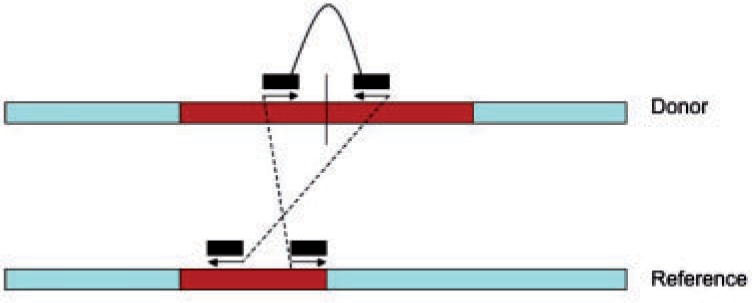
A discordant pair can imply the presence of a CNV.

2.1 Estimate copy-counts of repeat-rich regions

The formula to estimate copy-counts no longer works for repeat-rich regions. This is because the total number of reads mapped to the region is usually very different from the number of reads sequenced from the region. Since the region contains repeats which also occur elsewhere in the genome, the reads sequenced from all these repeats may be also mapped to the region and the reads sequenced from the region may be mapped to the repeats elsewhere. Without an accurate number of reads mapped to the region, the formula cannot estimate the copy-counts correctly.

To address the problem, we first identify the forward clusters of the forward reads {fo₁, fo₂,…,fo_m} and the backward clusters of the backward reads {ba₁, ba₂,…,ba_n}, where fo_i is the right most mapping position of the i-th forward cluster and ba_j is the left most position of the j-th backward cluster. Next we check all the candidate regions of [ba_j, fo_i] for all 1≤i≤m, 1≤j≤n, ba_j < fo_i. For each region, we obtain the total number of reads mapped to the region. As stated before, we cannot estimate the copy-counts directly using this number. Instead, for a region [ba_j, fo_i], we check all the mapping positions for each read sequenced from the genome, and count how many reads have mapping positions in the region. We denote the number of reads having mapping positions in the region as d. Then assume the read length is g, for every length g-mer in the region, we check all of its mapping positions in the genome that are not in the region. We sum the number of such mapping positions for all the length g-mers in the region and we denote the number as o. Therefore, there will be totally fl+o possible reads that may map to the region, where l=fo_i−ba_j. Given the coverage c, the number of reads that are expected to be sequenced from the donor CNV as well as the corresponding repeats is . All these reads will have mapping positions in the region [ba_j, fo_i]. Therefore, . Assume the copy-counts is f, then the Poisson likelihood function needs to be modified as where l=fo_i−ba_j. As we can see, fl approximates the length of the corresponding donor CNV for region [ba_j, fo_i], o approximates the sum of the length of all the corresponding repeats in the genome which are not contained but have occurrences in the region and d approximates the number of reads sequenced from the region as well as from all the corresponding repeats. Therefore, this modified formula is a natural extension of the original Poisson formula when the same mapping algorithm is used to map the reads to the reference and is able to estimate the copy-counts f correctly. To our knowledge, this is the first method that is able to estimate the copy-counts of CNVs in repeat-rich regions.

For illustration purpose, we show a simple example: assume the reference sequence contains three identical copies of a repeat of length 135 bp. For simplicity, we consider l=100 since any read sequenced from the last 35 bp of the repeat would not map to the repeat. One of the repeats is a candidate CNV region [ba_j, fo_i]. The repeat is copied one more time in the donor sequence, thus f=2. Let us simply assume the sequencer generates reads for each 36mer of the repeat, where each repeat generates hundred 36mers, thus c=36. Therefore, there can be totally 400 reads mapped to the reference CNV region, where the true number of reads sequenced from the donor CNV should be only 200 bp. Thus, the number of reads mapped to the reference CNV region may be very different from the number of reads sequenced from the donor CNV. However, if we use the above strategy to count the number of reads that have mapping positions in the reference CNV region, the number d is 400. Then next for each 36mer in the reference CNV region, we check all of its mapping positions in the genome that are not in the region. And we know each 36mer in the reference CNV has two mapping positions that are not in the region since the repeat has three identical copies. Therefore o, the sum of the number of such mapping positions for all 36mer in the region is 200. As we know, the Poisson likelihood function works when the number of reads mapped to a region is indeed the same as or similar to the number of reads sequenced from the region. Since we have only when f=2, the new Poisson likelihood function is able to accurately estimate the copy-counts.

2.2 Categorize occurrences of CNVs in repeat-rich regions

The repeats in the reference genome can also introduce significant confusions in identification of the internal junctions. For example, assume the reference sequence is ‘ACTGCAACTGCA’, the donor sequence is ‘ACTGCA GCA CTGCA ACTGCA’, the reference CNV ‘ACTGCA’ is copied three times in the donor sequence as ‘ACTGCA’, ‘GCA’ and ‘CTGCA’, respectively. If we have a paired-end read ‘CTG - - GCA’ spanning the first and the second copies (for illustration purpose, we assume each segment of the paired-end reads is of length 3 and the insert length, or the length of ‘-’, is also 2), when we map the read back to the reference sequence, since the two segments of the paired-end reads are mapped individually, we may end up with multiple mapping positions since ‘GCA’ can be mapped to both positions 4 and 10 and ‘CTG’ can be mapped to both positions 2 and 8. How do we determine which positions are the true mapping positions that can generate this read?

To answer the above question, we first categorize the occurrence of a CNV into one of the following three categories:

1. The reference CNV is in a non-repeat region such that the internal junctions as well as the left most and the right most boundaries can be identified uniquely using the clustered discordant paired-end reads.

2. Middle area of the reference CNV is in the repeat-rich region. More specifically, the left-most and the right-most boundaries of the CNV region can be identified uniquely. However, due to repeats in the middle of the CNV region, some or all of the internal junctions cannot be identified uniquely and there may be multiple mapping positions for the internal junctions. In this case, we need to identify the correct mapping positions for the internal junctions. For example, the reference sequence is ‘ACTGAGACTCTAT’, the donor sequence is ‘AC TGAGACTCTA TGAGA CTCTA T’, the reference CNV is ‘TGAGACTCTA’ and it contains repeats ‘GAGA’ and ‘CTCT’.

3. The whole reference CNV is in the repeat region such that at least one of the left and the right most boundaries and some or all of the internal junctions cannot be identified uniquely. For example, the reference sequence is ‘ACTGTGAGACTCTATAT’, the donor sequence is ‘ACTG TGAGACTCTA TGAGA CTCTA TAT’, the reference CNV is ‘TGAGACTCTA’ and it contains repeats ‘GAGA’ and ‘CTCT’. What is more, the length 2 substrings ‘TG’ and ‘TA’ at the left most boundary and right most boundary, respectively, also have duplicates in the reference sequence (in ‘ACTG’ and ‘TAT’, respectively).

2.3 Algorithms for CNV reconstruction in repeat-rich regions

We next develop different algorithms to handle each category according to their unique properties.

2.3.1 The reference CNV is in non-repeat region

In this case, all the donor CNV junctions are mapped uniquely to the reference CNV, which can be uniquely identified and we do not have any false positive mapping positions. So we can identify these positions and reconstruct the donor CNV easily.

2.3.2 Middle area of the reference CNV is in the repeat region

In this case, we assume that the left most and the right most boundaries of the reference CNV are not in the repeat region and can be identified uniquely. However, repeats within the reference CNV lead to possible multiple mapping positions for the remaining donor CNV junctions, namely the two segments of a discordant paired-end reads can be mapped to multiple places in the reference CNV due to repeats. In order to reconstruct the CNV, we need to identify the correct mapping positions of the junctions. This cannot be achieved alone by clustering discordant paired-end reads, since there will be multiple clusters at different positions for the same junction.

We solve the problem by estimating the length of the donor CNV first and then select one mapping position for each junction such that the reconstructed donor CNV has length closest to the estimated length. We estimate the length of the donor CNV using the number of reads that have mapping positions in the reference CNV. Since the left most and the right most boundaries of the reference CNV can be identified uniquely, we can find out the total number of reads having mapping positions in this region. As we showed before, the reads are generated with a Poisson distribution with respect to the length of the region l and the coverage ratio c. Given the total number of reads d having mapping positions in the reference CNV region, we have shown where f is the copy-counts, o is the sum of the number of mapping positions out of the reference CNV region for all length(read)-mer in the reference CNV region. Therefore, we can consequently estimate the length of the donor CNV region as 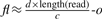. We can also estimate the copy-counts according to the process we described in the previous section using the formula . The number of mapping positions needs to be selected are then determined by the copy-counts. The problem of selecting the correct mapping positions is formalized with the following:

Problem 1. —

Given an estimate length l of the donor CNV, the position of the left most boundary b and the position of the right most boundary e, the copy-counts f, a set of n candidate junctions J=[e₁|b₁, e₂|b₂,…,e_n|b_n], select f−1 junctions F=[e_i1|b_i1, e_i2|b_i2,…,e_if−1|b_if−1] from the set J such that ‖Length(F, b, e)−l‖ is minimized, where Length(F, b, e)=(e_i1−b)+(e_i2−b_i1)+…+(e_if−1−b_if−2) + (e−b_if−1)=(e_i1−b)+∑_j=2^f−1(e_ij−b_ij−1)+(e−b_if−1).

A naive algorithm requires full enumeration of all the possible f−1 junctions from the set J, whose complexity is . Given n is usually as big as a few hundred to thousand, this complexity becomes too expensive to reconstruct a single CNV even for small f. Therefore, we design the following branch and bound algorithm to alleviate the expensive computation for solving the above problem.

We consider the junctions as nodes in a search tree. We randomly select a junction and then select one more junction at each step in a depth-first search manner. For any set of selected junctions, we derive an upper bound as well as a lower bound for Length(F, b, e) which we show are not dependent on the order of the junctions. The two bounds are updated at each step of the search process. Based on these two bounds, a lower bound for the function ‖Length(F, b, e)−l‖ is derived. A standard branch and bound algorithm is then applied to efficiently select the optimal set of junctions. Once a set of f−1 junctions are selected, or we reach a leaf node of the search tree, the upper bound of search tree is updated as the value of ‖Length(F, b, e)−l‖ which is then used to prune branches of the search tree. The upper bound is updated once a new leaf node is reached and a lower value of ‖Length(F, b, e)−l‖ is obtained. The algorithm stops till there is no more branch to be explored. We next prove a set of lemmas used to design the branch and bound algorithm.

Given a set F=[e_i1|b_i1, e_i2|b_i2,…, e_if−1|b_if−1], an order of junctions in F is [e_j1|b_j1, e_j2|b_j2,…,e_jf−1|b_jf−1] such that there is an one-to-one mapping from j_h to i_t for h, t ∈ {1,…,f−1} and j_h, i_t can be different. We call j_h an order index for the corresponding junction. The order of the junctions indicates the order of the copies of donor CNV and there are totally (f−1)! different orders. We first show an important property of the function Length(F, b, e) with respect to the order of the junctions.

Lemma 1. —

The order of junctions in F does not affect Length(F, b, e).

Proof. —

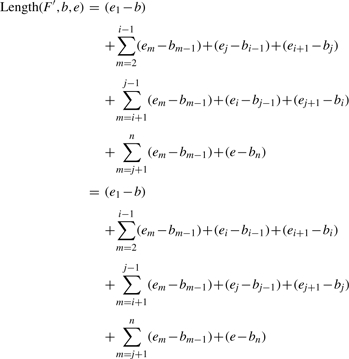
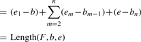
Since one order of junctions can be converted to any other different orders by continuously swapping the order index of two junctions each time, we just need to show this swapping operation does not change Length(F, b, e). Assume we have one order F=[…, e_i|b_i,…,e_j|b_j,…] and another order F′=[…, e_j|b_j,…,e_i|b_i, …], where the only difference between F and F′ is that the order index of e_i|b_i and e_j|b_j is swapped. Then assume F contains totally n junctions:

Therefore, the order of junctions in F does not affect Length(F, b, e).

We next show that we can derive an upper bound as well as a lower bound for Length(F, b, e) given any subset junctions of F.

Lemma 2. —

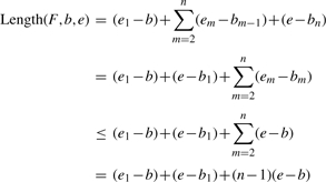
The upper bound of Length(F,b,e) is (e₁−b)+∑_m=2^k(e_m−b_m−1)+(e−b_k)+(n−k)(e−b) given the size of F is n, a subset of selected junctions as F′=[e₁|b₁, e₂|b₂,…,e_k|b_k], where k ≤ n.

Proof. —

We prove this lemma by induction. When the subset is of size 1, assume F′=[e₁|b₁], then we need to select n−1 more junctions.

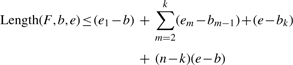
Similarly, when the subset is of size k, assume F′=[e₁|b₁, e₂|b₂,…,e_k|b_k], we have

 ▪

The same idea can be applied to derive the lower bound of Length(F,b,e).

Lemma 3. —

The lower bound of Length(F,b,e) is (e₁−b)+∑_m=2^k(e_m−b_m−1)+(e−b_k) given the size of F is n, and a subset of selected junctions as F′=[e₁|b₁, e₂|b₂,…,e_k|b_k], where k≤n.

Proof. —

The proof is done by induction and is similar to that of Lemma 2. We omit the proof here.

Similarly, when the subset is of size k, assume F′=[e₁|b₁,e₂|b₂,…,e_k|b_k], we have

 ▪

Given the upper bound up and the lower bound lo of Length(F, b, e), we can compute a lower bound δ′ for δ=‖Length(F, b, e)−l‖ as the following: (i) if lo ≤l≤up, δ′=0. (ii) If l≤lo, δ′=lo−l. (iii) If l≥up, δ′=l−up. Therefore, we can apply the standard branch and bound algorithm to select the set of junctions which minimize δ. Our experiments show later that this branch and bound algorithm is much more efficient than the naive algorithm.

The above algorithm is able to select an optimal set of junctions to minimize the objective function ‖Length(F,b,e)−l‖. However, this does not guarantee the selected junctions are the true junctions. This is because the estimated length is very close but usually not exactly the same as the true CNV length, since the estimated length is based on a limited amount of reads generated from the reference CNV region. Also the false positive positions of the donor junctions maybe selected by the above process, if some combination of them leads to the minimum difference between the estimated length and the reconstructed CNV length. Our experiments on simulated data show that on general the above process works pretty well even with these two limitations.

In Problem 1, Length(F,b,e) is the length of the donor CNV based on our assumption b₁=b and e_f=e. Without this assumption, we can use discordant reads to identify the mapping positions for the left most junction containing b₁ and the right most junction containing e_f between the donor CNV and the genome. Then we can include these mapping positions in the candidate junction set J. All of the above lemmas and algorithms can be easily adapted to handle this more general problem. Due to space limit, we do not show the generalization of the above algorithm.

2.3.3 The whole reference CNV is in the repeat region

When the left most boundary and the right most boundary of the reference CNV also have multiple mapping positions in the reference genome, the algorithm discussed in the previous section cannot be applied directly. This is because we cannot estimate the length of the donor CNV without knowing the true boundaries of the region. Therefore, we need to first identify the true boundaries of the reference CNV.

Unfortunately, we are not able to uniquely identify the true boundaries since they are mapped to multiple places in the reference genome. Therefore, the best we can do is to find a pair of mapping positions for the left most and right most boundaries and a copy-count value such that the reconstructed CNV has length closest to the estimated length, which is again . Assuming the left most boundary is mapped to n positions in the reference genome, while the right most boundary is mapped to m positions in the reference genome, the problem can be formalized with the following:

Problem 2. —

Given the set of mapping positions for the left most boundary B={b₁,b₂,…,b_n}, where b₁<b₂<…<b_n, and the set of mapping positions for the right most boundary E={e₁,e₂,…,e_m}, where e₁<e₂<…<e_m, select a pair (b_i,e_j) and a copy-counts f such that Dist(B,E,f,L,b_i,e_j)=‖(f−1)×(e_j−b_i)+(e_m−b₁)−L‖ is minimized for all 1≤i≤n, 1≤j≤m and f≥2, where L is the estimated length of the donor CNV.

We need to check all O(n×m) pairs to find the pair (b_i,e_j) minimizing Dist(B,E,f,L,b_i,e_j). A naive method requires checking all O(n×m) pairs and testing many u≥2 for each pair until the best copy-counts is found. But in reality, most of these searches can be pruned.

We next design a more efficient algorithm. We try to select the length of the CNV, determined by the two boundaries, as well as the copy-counts at the same time. The selection process can be terminated a lot faster, based on our observation that to minimize Dist(B,E,f,L,b_i,e_j), the copy-counts needs to remain the same or decrease when the length of the CNV increases. Therefore, we start our search from short CNV to long CNV, and decrease the copy-counts continuously until the copy-counts is less than 2, which is the stop criterion of the search process.

The algorithm works with the following lemma:

Lemma 4. —

Given a pair (b_i, e_j), f=argmin_fDist(B,E,f,L,b_i,e_j) and a pair (b_i^′,e_j^′), f′=argmin_fDist(B,E,f,L,b_i^′,e_j^′) and e_j-b_i≤e_j^′−b_i^′, Dist(B,E,f′,L,b_i^′,e_j^′)≤Dist(B,E,f,L,b_i,e_j), we must have f′≤f.

Proof. —

We prove the lemma by contradiction. For the pair (b_i, e_j) and f=argmin_fDist(B,E,f,L,b_i,e_j), there are two cases:

1. f is the minimum copy-counts such that (f−1)×(e_j−b_i)+(e_m−b₁)≥L. Then Dist(B,E,f,L,b_i,e_j)=(f−1)×(e_j−b_i)+(e_m−b₁)−L. Now assume f′>f, given e_j−b_i≤e_j^′−b_i^′, we have Dist(B,E,f′,L,b_i^′,e_j^′)=(f′−1)×(e_j^′−b_i^′)+(e_m−b₁)−L > (f−1)×(e_j−b_i)+(e_m−b₁)−L=Dist(B,E,f,L,b_i,e_j), which is contradicted with Dist(B,E,f,L,b_i^′,e_j^′)≤Dist(B,E,f,L,b_i,e_j). Therefore, we can only have f′≤f.

2. f is the maximal copy-counts such that (f−1)×(e_j−b_i)+(e_m−b₁)≤L. Then we must have f×(e_j−b_i)+(e_m−b₁)>L. Since f=argmin_fDist(B,E,f,L,b_i,e_j), we must also have Dist(B,E,f,L,b_i,e_j)≤Dist(B,E,f+1,L,b_i,e_j). Given e_j−b_i≤e_j^′−b_i^′, we have f×(e_j^′−b_i^′)+(e_m−b₁)≥f×(e_j−b_i)+(e_m−b₁)≥L. Therefore, Dist(B,E,f+1,L,b_i^′,e_j^′)≥Dist(B,E,f+1,L,b_i,e_j)≥Dist(B,E,f,L,b_i,e_j). Now assume f′>f, namely f′≥f+1, we have Dist(B,E,f′,L,b_i^′,e_j^′)≥Dist(B,E,f+1,L,b_i^′,e_j^′)≥Dist(B,E,f,L,b_i,e_j) which is contradicted with Dist(B,E,f′,L,b_i^′,e_j^′)≤Dist(B,E,f,L,b_i,e_j). Therefore, we can only have f′≤f.

The above lemma suggests that we can first identify a minimum overlapping region, which is the region that does not contain any subregion. For example, for b₁<e₁<b₂<e₂, the minimum overlapping regions are [b₁,e₁] and [b₂,e₂]. [b₁,e₂] is not a minimum overlapping region since it contains a subregion [b₁,e₁]. Since the region is actually a 1D interval, this can be done easily by finding the biggest b_i for each e_j such that b_i<e_j and the minimum overlapping regions are all such (b_i,e_j)'s for each e_j. Then we can expand the regions in both directions to bigger regions. During the expansion process, the best copy-counts for each region can only remain the same or decrease. Once the copy-counts drop to below 2, we can stop the expansion. Since there are multiple minimum overlapping regions, we can start with the shortest one and we repeat the expansion process from each minimum overlapping region until we have checked all O(n×m) regions.

Once we find a pair (b_i,e_j) and a copy-count f such that Dist(B,E,f,L,b_i,e_j) is minimized, we can apply the branch and bound algorithm discussed in the previous section to identify all the internal junctions.

2.4 Reconstruction of CNVs

As shown in Lemma 1, the order of junctions does not affect the length of the donor CNV. Therefore, for a given set of junctions minimizing Length(F,b,e), we cannot determine their true orders in the donor CNV since all these orders are equally likely given the reads generated from the donor CNV. To reconstruct the donor CNV, we can simply select a random order of these junctions which leads to a corresponding reconstructed donor CNV.

3 EXPERIMENTAL RESULTS

3.1 Experiments on mouse genome

In this part of the article, we will illustrate the power of our method on real data. We used the data published by Sudbery et al. (2008) where they sequenced the chromosome 17 of A/J mouse strain (95 Mb), using the Illumina technology (Sudbery et al., 2008). Chromosome 17 is biologically interesting for two main reasons. First, mouse major compatibility complex (MHC) resides on this chromosome (Ohtsuka et al., 2008). Second, murine t-complex also resides in chromosome 17 which in some wild-derived strains is responsible for transmission ration disorder (Bauer et al., 2005). There are totally 56 019 759 paired-end reads sequenced and each segment of the paired-end read is 36 bp long which makes the data has 22× coverage. The average insert length of the paired-end reads is around 120 bp. Due to the fact, we need all possible mapping locations [as indicated in previous studies (Alkan et al., 2009; Hormozdiari et al., 2009; Lee et al., 2009; Medvedev et al., 2009, 2010) for detecting CNV and SV, it is essential to use all the possible mapping positions] for each read, we map the reads using mrFAST (Alkan et al., 2009; Hach et al., 2010). In the mapping, we used the C57BL/6J (NCBI m37) as the reference to map the reads. The threshold of read mapping was set to e≤2 edit distance (allowing reads mapped with up to two mismatches and indels) in which reads will map to locations with sequence similarity higher than 94% (in all previous studies dealing with 36 bp Illumina short reads, threshold of two mismatches is used). Lots of reads have multiple mapping positions and there are totally more than 8 billion mapping positions for these reads.

By using the discordant reads, we identify candidate regions for CNVs of category two and three. In this work, for simplicity, we limit the length of the region within the range of (1–10 kb). When we cluster the discordant reads, we require two adjacent reads in the same cluster overlap with each other. We also require the insert length for a paired-end read after being mapped to the reference sequence be greater than 500 bp to be considered as discordant such that each copy is long enough. We only use clusters of reads with size greater than 7 to identify the candidate CNV regions. There 381 candidate regions for CNVs of category two, where the left most and the right most boundaries are determined by clusters of reads with unique mapping positions. We estimate the copy-counts of these regions using the modified Poisson likelihood function and we identify a total of five regions with copy-counts not less than 2. One of these regions overlaps with the CNV regions reported by Sudbery et al. (2008), and four of them are new regions.

To further validate the four new regions, we apply our algorithm to reconstruct the CNVs. To our knowledge, there is no annotation of existing CNVs in repeat-rich regions, and we are not able to evaluate the accuracy of the reconstruction directly from any known literature. Therefore, we validate our reconstruction using unmapped reads, which are reads that do not map to the reference sequence, mainly due to two reasons: (i) the reads contain sequencing errors; (ii) the reads span the breakpoints of some structural variations. We say an unmapped read supports a breakpoint if it spans the breakpoint. To check if an unmapped read spans a breakpoint, similar to the work in He et al. (2010), we split the unmapped read into two substrings, and map both substrings to the two sides of the breakpoints. If both substrings match the corresponding side of the breakpoint, we say the unmapped read supports the breakpoint. However, the reconstructed breakpoints may be a little bit off from the true breakpoint due to the effects of reads mapping, clustering of the discordant reads, etc. Therefore, we also check a 200 bp neighborhood of the breakpoints. If the two split substrings of an unmapped read maps to the neighborhood, we still consider the read supports the breakpoint. Then for each reconstructed breakpoint, we check the number of unmapped reads supporting it. Given the coverage as 22 times, the expected number of reads spanning any position in the genome, including breakpoints, is 22. In Figure 2, we show the averaged number of unmapped reads supporting the breakpoints in each of the five regions and their corresponding copy-counts. As we can see, for most of the regions, the number of unmapped reads supporting the breakpoints is very close to the expected number 22, indicating that these regions and breakpoints are highly possible to be true. To further evaluate the performance of our reconstruction algorithms, we next conducted experiments on simulated sequences.

Fig. 2.

Averaged number of unmapped reads supporting the breakpoints in each of the five regions and their corresponding copy-counts.

3.2 Experiments on simulated sequences

As mentioned earlier, to our knowledge, there is no annotation of exact internal junctions of existing CNVs in repeat-rich regions, so to illustrate the performance of the algorithms we proposed, we also test our methods on simulated genome sequences. We conduct a set of experiments for each of the three cases with respect to different parameter. We first randomly generate a genome sequence which does not contain any long repeats. Then we insert CNVs at random positions in the simulated sequence. For case one, the reference CNV regions, prefixes and suffixes of the donor CNV copies as well as copy-counts are randomly generated. For case two, where the middle area of the reference CNV region contains repeats, we first randomly select the reference CNV region. Next, we randomly sample pre-masked repeat sequences from the RepeatMasker web site (RepeatMasker, 2010) and insert these repeat sequences multiple times into the reference CNV region, avoiding the left most and right most boundaries. Finally, the prefixes and suffixes of the donor CNV copies are randomly generated. This process guarantees that the left most and right most boundaries of the reference CNV can be identified uniquely, while the internal junctions may fall within the repeat region. For case three, the simulation process is almost identical to the one for case two, with the only difference being that we insert repeats first and then randomly generate CNVs within repeat regions. For all experiments, we set the coverage ratio to 40 times, read length to 36 bp and insert length within the range of 90–100 bp. We do not compare our method with any other existing CNV detection methods using HTS technologies since none of them is able to handle CNVs in repeat-rich regions and also none of them is publicly available.

Since for category one, we are always able to identify the internal junctions uniquely, we do not show the experimental results here.

3.2.1 Middle area of the reference CNV is in the repeat region

For the category two experiments, we construct repeat-rich regions by duplicating a repeat sequence, which is randomly sampled from RepeatMasker, eight times, which is able to introduce enough complexes on the repeat structures. We set the copy-counts to 4 so that the number of mapping positions for each internal junction will be large. The above parameters are chosen just to make sure the problem is hard enough to show the advantage of our algorithm over the naive algorithm. Then we evaluate the performance of our branch and bound algorithm with respect to the length of the reference CNV region. The longer the reference CNV is, the more mapping positions the CNV is expected to have and the harder the reconstruction problem is. We vary the length of the reference CNV region as 10 000, 5000 and 2500 bp. The experimental results are shown in Figures 3 and 4. For each reference CNV length, we show the averaged results of our algorithm on 10 experiments.

Fig. 3.

The efficiency evaluation of the branch and bound algorithm (BB) versus the full enumeration of all possible orders for reference CNV of different length. All the results are averaged on 10 experiments.

Fig. 4.

The accuracy evaluation of the branch and bound algorithm for reference CNV of different length. All the results are averaged on 10 experiments.

In Figure 3, we illustrate the efficiency of our branch and bound algorithm. We first show the total number of mapping positions for the internal junctions. As we can see, as the size of the reference CNV increases, the number of mapping positions increases and the Problem 1 becomes more difficult. We also show the number of orders searched by our branch and bound algorithm and by the full enumeration and their ratio. The branch and bound algorithm has significant advantages over the full enumeration, especially for the length 10 000 bp case, where our branch and bound algorithm only searches 0.019% of the orders of the full enumeration. Given this dramatic advantage, our algorithm has very short run times for all cases, while the run times of full enumeration are too long so we do not show them here.

In Figure 4, we show our algorithm is not only efficient but also accurate. We compare the estimated internal junctions with the true internal junctions. If the difference is <100 bp, which is the maximal insert length we use in our experiments, we consider the estimation as accurate. As we can see, with relatively short reference CNVs, our estimations are very accurate, especially for reference CNVs of size 2500 bp. This is because the number of mapping positions is small for short reference CNV regions, as shown in Figure 3, and for short reference CNV regions, the mapping positions tend to be close to each other. For cases where our algorithm makes incorrect estimations, we show that these estimations are still much better than random guesses. To illustrate this, we show the averaged distances between our estimated internal junctions and the true internal junctions, and the averaged distances between all possible mapping positions and the true internal junctions, which can be considered as the distance of random sampled positions. We measure the distance between the starting positions and the ending position separately and these distances are rounded into integers. As illustrated in Figure 4, the distances of our estimated junctions are only 1% of the distances of the random samples. Therefore, even though our algorithm may fail to estimate the true internal junctions, the estimations are still very close to the true junctions.

We also test our algorithm for other parameter settings, such as different copy-counts, different repeat sequence duplication times, etc., and we obtain similar results. Due to space limit, we do not show the results for other parameter settings.

3.2.2 The whole reference CNV is in the repeat region

For the experiments on category three, we evaluate the performance of our pruning strategy with respect to the similar parameters as those for case two. In this experiment, we set the reference CNV length as 10 000 bp, the copy-counts as 4, and we vary the times we duplicate the repeat sequence sampled from RepeatMasker to create different levels of repeat-richness. We vary the repeat sequence duplication time as 1, 5, 10, 20, 30. The more times the sequence is duplicated, the more mapping positions the CNV is expected to have and thus the harder the problem is. In order to avoid noise, we only search for CNV regions above certain length threshold. This is because if we allow searching for short CNV regions, the short CNV regions tend to dominate the search since they are more likely to minimize the function defined in Problem 2. The most extreme case is when a CNV region is of length 1, the function will always be minimized by this CNV. Therefore, we use a relatively large threshold 8000 bp. This indicates that if we roughly know the length of the CNVs, our algorithm has better chance to identify them. Also we only insert one CNV for each repeat-rich region, which contains all duplications for the same repeat sequence. The experimental results are shown in Figure 5. All the results are averaged on 10 experiments.

Fig. 5.

The performance evaluation of the pruning algorithm for reference CNV of length 10 000 bp, copy-counts 4 and the repeat sequence duplication time as 1, 5, 10, 20, 30. All the results are averaged on 10 experiments. The numbers are all rounded.

We compare the number of searches by the pruning and non-pruning algorithm. As we can see, as the repeat-richness increases, the advantage of the pruning algorithm over the non-pruning algorithm becomes more significant. When we duplicate the repeat sequence 20 and 30 times, the pruning algorithm only makes <0.5% of the searches made by the non-pruning algorithm. As a consequence, the run time of the pruning algorithm is always <0.5 s while the run time of the non-pruning algorithm increases sharply as the repeat-richness increases. Again, to evaluate the accuracy of our method, we compare the distance between the estimated pair of boundaries to the true pair of boundaries. We compare this distance with the average distance of all pairs of positions satisfying the length threshold, which can be considered as the distance of randomly sampled pairs of boundaries. Our estimation is not very accurate, compared to the internal junction estimation for category two. But it is still a lot better than randomly sampled boundaries. Also our method is able to estimate the copy-counts always correctly while the copy-counts estimation from the randomly sampled pairs is almost always wrong.

4 DISCUSSION AND FUTURE WORK

In this study, we proposed an efficient branch and bound algorithm as well as a pruning strategy to identify and reconstruct tandem CNVs in repeat-rich regions. To our knowledge, our method is the first attempt to recover CNVs in repeat-rich regions. Our experiments show that our method is not only efficient but also accurate. However, there is still lots of room to improve, for example, when there are multiple CNVs in the same repeat-rich region, the estimation of the CNV length becomes much more complicated, especially when CNVs overlap with each other. It is not clear that whether the CNVs can be identified and reconstructed for these more complicated cases. But our article proposed a framework that shed light on the possible solutions for the more complicated cases.

Funding: D.H., F.H., N.F. and E.E. are supported by National Science Foundation grants 0513612, 0731455, 0729049 and 0916676, and NIH grants K25-HL080079 and U01-DA024417. N.F. is supported by NIH training grant T32-HG002536. This research was supported in part by the University of California, Los Angeles subcontract of contract N01-ES-45530 from the National Toxicology Program and National Institute of Environmental Health Sciences to Perlegen Sciences.

Conflict of Interest: none declared.

REFERENCES

- Aitman T., et al. Copy number polymorphism in Fcgr3 predisposes to glomerulonephritis in rats and humans. Nature. 2006;439:851–855. doi: 10.1038/nature04489. [DOI] [PubMed] [Google Scholar]
- Alkan C., et al. Personalized copy number and segmental duplication maps using next-generation sequencing. Nat. Genet. 2009;41:1061–1067. doi: 10.1038/ng.437. [DOI] [PMC free article] [PubMed] [Google Scholar]
- Bauer H., et al. The t complex-encoded GTPase-activating protein Tagap1 acts as a transmission ratio distorter in mice. Nat. Genet. 2005;37:969–973. doi: 10.1038/ng1617. [DOI] [PubMed] [Google Scholar]
- Chen P., et al. CNVDetector: locating copy number variations using array CGH data. Bioinformatics. 2008;24:2773. doi: 10.1093/bioinformatics/btn517. [DOI] [PubMed] [Google Scholar]
- Chiang D., et al. High-resolution mapping of copy-number alterations with massively parallel sequencing. Nat. Methods. 2009;6:99. doi: 10.1038/nmeth.1276. [DOI] [PMC free article] [PubMed] [Google Scholar]
- Daruwala R., et al. A versatile statistical analysis algorithm to detect genome copy number variation. Proc. Natl Acad. Sci. USA. 2004;101:16292. doi: 10.1073/pnas.0407247101. [DOI] [PMC free article] [PubMed] [Google Scholar]
- Gonzalez E., et al. The influence of CCL3L1 gene-containing segmental duplications on HIV-1/AIDS susceptibility. Science. 2005;307:1434. doi: 10.1126/science.1101160. [DOI] [PubMed] [Google Scholar]
- Hach F., et al. mrsFAST a cache-oblivious algorithm for short-read mapping. Nat. Methods. 2010;7:576–577. doi: 10.1038/nmeth0810-576. [DOI] [PMC free article] [PubMed] [Google Scholar]
- He D., et al. Detection and reconstruction of tandemly organized de novo copy number variations. BMC Bioinformatics. 2010;11(Suppl. 11):S12. doi: 10.1186/1471-2105-11-S11-S12. [DOI] [PMC free article] [PubMed] [Google Scholar]
- Hormozdiari F., et al. Combinatorial algorithms for structural variation detection in high throughput sequenced genomes. Genome Res. 2009;19:1270–1278. doi: 10.1101/gr.088633.108. [DOI] [PMC free article] [PubMed] [Google Scholar]
- Lai W., et al. Comparative analysis of algorithms for identifying amplifications and deletions in array CGH data. Bioinformatics. 2005;21:3763. doi: 10.1093/bioinformatics/bti611. [DOI] [PMC free article] [PubMed] [Google Scholar]
- Lee S., et al. MoDIL: detecting small indels from clone-end sequencing with mixtures of distributions. Nat. Methods. 2009;6:473–474. doi: 10.1038/nmeth.f.256. [DOI] [PubMed] [Google Scholar]
- Lucito R., et al. Representational oligonucleotide microarray analysis: a high-resolution method to detect genome copy number variation. Genome Res. 2003;13:2291. doi: 10.1101/gr.1349003. [DOI] [PMC free article] [PubMed] [Google Scholar]
- Medvedev P., et al. Computational methods for discovering structural variation with next-generation sequencing. Nat. Methods. 2009;6:S13–S20. doi: 10.1038/nmeth.1374. [DOI] [PubMed] [Google Scholar]
- Medvedev P., et al. Detecting copy number variation with mated short reads. Genome Res. 2010;20:1613–1622. doi: 10.1101/gr.106344.110. [DOI] [PMC free article] [PubMed] [Google Scholar]
- Ohtsuka M., et al. Major histocompatibility complex (mhc) class ib gene duplications, organization and expression patterns in mouse strain c57bl/6. BMC Genomics. 2008;9:178. doi: 10.1186/1471-2164-9-178. [DOI] [PMC free article] [PubMed] [Google Scholar]
- RepeatMasker (2010) RepeatMasker. Available at http://www.repeatmasker.org/(last accessed date April 16, 2011).
- Sebat J., et al. Strong association of de novo copy number mutations with autism. Science. 2007;316:445. doi: 10.1126/science.1138659. [DOI] [PMC free article] [PubMed] [Google Scholar]
- She X., et al. Mouse segmental duplication and copy-number variation. Nat. Genet. 2008;40:909. doi: 10.1038/ng.172. [DOI] [PMC free article] [PubMed] [Google Scholar]
- Simpson J.T., et al. Copy number variant detection in inbred strains from short read sequence data. Bioinformatics. 2010;26:565–567. doi: 10.1093/bioinformatics/btp693. [DOI] [PMC free article] [PubMed] [Google Scholar]
- Sudbery I., et al. Deep short-read sequencing of chromosome 17 from the mouse strains a/j and cast/ei identifies significant germline variation and candidate genes that regulate liver triglyceride levels. Genome Biol. 2008;10:R112. doi: 10.1186/gb-2009-10-10-r112. [DOI] [PMC free article] [PubMed] [Google Scholar]