Sparse Regulatory Networks

Abstract

In many organisms the expression levels of each gene are controlled by the activation levels of known “Transcription Factors” (TF). A problem of considerable interest is that of estimating the “Transcription Regulation Networks” (TRN) relating the TFs and genes. While the expression levels of genes can be observed, the activation levels of the corresponding TFs are usually unknown, greatly increasing the difficulty of the problem. Based on previous experimental work, it is often the case that partial information about the TRN is available. For example, certain TFs may be known to regulate a given gene or in other cases a connection may be predicted with a certain probability. In general, the biology of the problem indicates there will be very few connections between TFs and genes. Several methods have been proposed for estimating TRNs. However, they all suffer from problems such as unrealistic assumptions about prior knowledge of the network structure or computational limitations. We propose a new approach that can directly utilize prior information about the network structure in conjunction with observed gene expression data to estimate the TRN. Our approach uses L₁ penalties on the network to ensure a sparse structure. This has the advantage of being computationally efficient as well as making many fewer assumptions about the network structure. We use our methodology to construct the TRN for E. coli and show that the estimate is biologically sensible and compares favorably with previous estimates.

1. Introduction

Recent progress in genomic technology allows scientists to gather vast and detailed information on DNA sequences, their variability, the timing and modality of their translation into proteins, and their abundance and interacting partners. The fields of system and computational biology have been redefined by the scale and resolution of these data sets and the necessity to interpret this data deluge. One theme that has clearly emerged is the importance of discovering, modeling and exploiting interactions among different biological molecules. In some cases, these interactions can be measured directly, in others they can be inferred from data on the interacting partners. In this context, reconstructing networks, analyzing their behavior and modeling their characteristics have become fundamental problems in computational biology.

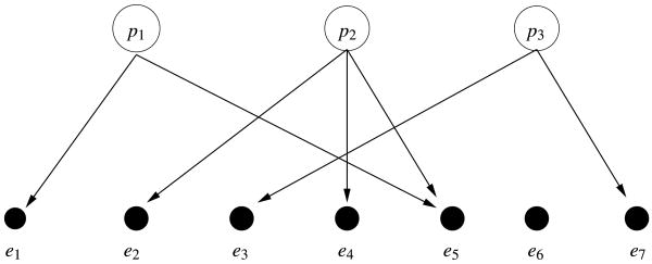
Depending on the type of biological process considered, and the type of data available, different network structures and graph properties are relevant. In this work we focus on one type of bipartite network that has been used to model transcription regulation, among other processes, and is illustrated in Figure 1. One distinguishes input nodes (p₁, p₂, p₃ in Figure 1) and output nodes (e₁, …, e₇ in Figure 1); directed edges connect input nodes to one or more output nodes and indicate control. Furthermore, we can associate a numerical value with each edge, which indicates the nature and strength of the control.

Fig. 1.

A general network with L = 3 transcription factors and n = 7 genes.

Bipartite networks such as the one illustrated in Figure 1 have been successfully used to describe and analyze transcription regulation [see, e.g., Liao et al. (2003)]. Transcription is the initial step of the process whereby the information stored in genes is used by the cell to assemble proteins. To adapt to different cell functions and different environmental conditions, only a small number of the genes in the DNA are transcribed at any given time. Understanding this selective process is the first step toward understanding how the information statically coded in DNA dynamically governs all the cell life. One critical role in the regulation of this process is played by transcription factors. These molecules bind in the promoter region of the genes, facilitating or making it impossible for the transcription machinery to access the relevant portion of the DNA. To respond to different environments, transcription factors have multiple chemical configurations, typically existing both in “active” and “inactive” forms. Their binding affinity to the DNA regulatory regions varies depending on the particular chemical configuration, allowing for a dynamic regulation of transcription. Depending on the complexity of the organism at hand, the total number of Transcription Factors (TF) varies, as well as the number of TF participating in the regulation of each gene. In bipartite networks such as the one in Figure 1, input nodes can be taken to represent the variable concentrations in active form of transcription factors, and output nodes as the transcript amounts of different genes. An edge connecting a TF to a gene indicates that the TF participates in the control of the gene transcription. As usual, mathematical stylization only captures a simplified version of reality. Bipartite graphs overlook some specific mechanisms of transcription regulation, such as self-regulation of TF expression or feed-back loops connecting genes to transcription factors. Despite these limitations, networks such as the one in Figure 1 provide a useful representation of a substantial share of the biological process.

Researchers interested in reconstructing transcription regulation have at their disposal a variety of measurement types, which in turn motivate diverse estimation strategies. The data set that motivated the development of our methodology consisted of measurements of gene transcription levels for E. coli, obtained from a collection of 35 gene expression arrays. These experiments, relatively cheap and fairly common, allow one to quantify transcription amounts for all the genes in the E. coli genome, under diverse cell conditions. While our data consists of measurements on the output nodes, that is, the gene expression levels, we also have access to some information on the topology of the network: DNA sequence analysis or ChIP–chip experiments can be used to evaluate the likelihood of each possible edge. However, we have no direct measurements of the input nodes, that is, the concentrations of active form of the TFs. While, in theory, it is possible to obtain these measurements, they are extremely expensive and are typically unavailable. Changes in transcription of TF are measured with gene expression arrays, but mRNA levels of transcription factors seldom correlate with changes in the concentration of their active form. The latter, in fact, are most often driven by changes in TF expression level only in response to the cell inner clock (i.e., in development, or in different phases of the cell cycle). We are interested in studying the cellular response to external stimuli and this is most frequently mediated by post-translational modifications of the TF. For these reasons, we are going to consider the concentrations of active forms of the TF as unobserved.

Our E. coli data consist of spotted array experiments with two dyes, which measure the changes in expression from a baseline level for the queried genes (taking the logarithm of the ratio of intensities, typically reported as raw data). These percentage changes can be related linearly to variations in the concentrations of active form of transcription factors, as documented in Liao et al. (2003). Coupling this linearity assumption, with the bipartite network structure, we model the log-transformed expressions of gene i in experiment t, e_it, as

$$e_{it}=\sum _{j=1}^L{a}_{ij}{p}_{jt}+{\varepsilon }_{it},i=1,\dots ,n,t=1,\dots ,T,$$

where n, L and T respectively denote the number of genes, TFs and experiments, a_ij represents the control strength of transcription factor j on gene i, p_jt the concentration of the active form of transcription factor j in experiment t, and ε_it captures i.i.d. measurement errors and biological variability. A value of a_ij = 0 indicates that there is no network connection or, equivalently, no relationship, between gene i and TF j, while nonzero values imply that changes in the TF affect the gene's expression level. It is convenient to formulate the model in matrix notation,

$$E=AP+\varepsilon ,$$ (1)

where E is an n × T matrix of e_it's, A is an n × L matrix of a_ij's and P is an L × T matrix of p_jt's. A and P are both unknown quantities.

Model (1), derived from the bipartite regulatory network and linearity assumption, is a very familiar one to statisticians and a number of its variants have been applied to the study of gene expression and other data. The first attempts utilized dimension reduction techniques such as principal component analysis (PCA) or singular value decomposition [Alter, Brown and Botstein (2000)]. Using this approach, a unique solution to simultaneously estimate the p_j 's and the strength of the network connections is obtained by assuming orthogonality of the p_j's—an assumption that does not have biological motivations. Some variants of PCA, that aim to produce more interpretable results, have also been studied. For example, Lee and Seung (1999, 2001) developed nonnegative matrix factorization (NNMF) where the elements of A and P are all constrained to be positive. However, for our data we would expect both positive and negative control strengths, so it does not seem reasonable to enforce the elements of A to be positive. An interesting development is the use of Independent Component Analysis [Lee and Batzoglou (2003)], where the orthogonality assumption is substituted by stochastic independence. These models can be quite effective in providing a dimensionality reduction, but the resulting p's often lack interpretability.

West (2003) treats (1) as a factor model and uses a Bayesian approach to reduce the dimension of expression data, paying particular attention to the development of sparse models, in order to achieve a biologically realistic representation. When the gene expression data refers to a series of experiments in a meaningful order (temporal, by degree of exposure, etc.), model (1) can be considered as the emission component of a state space model, where hidden states can be meaningfully connected to transcription factors [Beal et al. (2005), Li et al. (2006), Sanguinetti et al. (2006)]. Depending on the amount of knowledge assumed on the A matrix, state space models can deal with networks of different size and complexity.

Values of the factors, P, that are clearly interpretable as changes in concentration of the active form of transcription factors together with the identifiability of model (1) can be achieved by imposing restrictions on A that reflect available knowledge on the topology of the network. Liao et al. (2003) assumes the entire network structure known a priori and gives conditions for identifiability of A and P based on the pattern of zeros in A, reflecting the natural sparsity of the system. A simple iterative least squares procedure is proposed for estimation, and the bootstrap used to asses variability. This approach has two substantial limitations. First, it assumes that the entire network structure is known, while, in practice, it is most common for only parts of the structure to have been thoroughly studied. Second, not all known transcription networks satisfy the identifiability conditions. A number of subsequent contributions have addressed some of these limitations. Tran et al. (2005) introduces other, more general, identifiability conditions; Yu and Li (2005) proposes an alternative estimation procedure for the factor model; Brynildsen, Tran and Liao (2006) explores the effect of inaccurate specification of the network structure; Chang et al. (2008) proposes a faster algorithm. Pournara and Wernisch (2007) provides an informed review of the use of factor models for regulatory networks, surveying both different identifiability strategies and computational approaches.

Particularly relevant to the present paper is the work of Sabatti and James (2006), which removes both limitations of the Liao et al. (2003) method by using a Bayesian approach. The authors obtain a prior probability on the network structure using sequence analysis, and then use a Gibbs sampler to produce posterior estimates of the TRN. In theory, this approach can be applied to any network structure, even when only part of the structure is known. However, a significant limitation is that the computational effort required to implement the Gibbs sampler grows exponentially with the number of potential connections between a particular gene and the transcription factors. As a result, one is forced to choose a prior on the network where the probability of most edges is set to zero, thereby fixing a priori a large portion of the topology. While sparsity in the connections is biologically reasonable, it would obviously be more desirable to allow the gene expression data to directly identify the connections.

To overcome these limitations, in this paper we take a somewhat different approach that builds in the same advantages as the Bayesian method in terms of utilizing partial network information and working for any structure. However, our approach is more computationally efficient, which allows increased flexibility in determining the final network topology. We treat the estimation of both the connection strengths, A, and the transcription factors concentrations, P, as a variable selection problem. In this context, our data has an extremely large number of variables, that is, potential connections, but is sparse in terms of the number of “true” variables, that is, connections that actually exist. There have recently been important methodological innovations for this type of variable selection problem. A number of these methods involve the use of an L₁ penalty on the regression coefficients which has the effect of performing automatic variable selection. A few examples include the Lasso [Tibshirani (1996)], SCAD [Fan and Li (2001)], the Elastic Net [Zou and Hastie (2005)], the adaptive Lasso [Zou (2006)], the Dantzig selector [Candes and Tao (2007)], the Relaxed Lasso [Meinshausen (2007)], VISA [Radchenko and James (2008)] and the Double Dantzig [James and Radchenko (2009)]. The most well known of these approaches is the Lasso, which performs variable selection by imposing an L₁ penalty on the regression coefficients. In analogy with the Lasso, our method also utilizes L₁ penalties on the connection strengths, A, as well as the transcription factor concentrations, P. This allows us to automatically produce a sparse network structure, which incorporates the prior information. We show that, given the same prior network, our approach produces similar results to the Bayesian formulation, but is considerably more computationally efficient. This in turn allows us to reconstruct regulatory networks using less precise prior information.

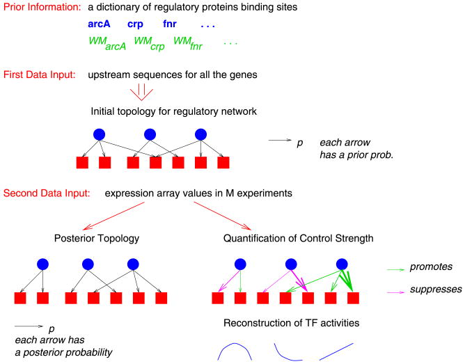
Figure 2 gives a schematic illustration of our approach. First, we identify a group of transcription factors that are believed to regulate the gene expression levels. Second, we compute an initial topology for the network using both documented experimental evidence, as well as an analysis of the DNA sequence upstream of a given gene. Finally, we use the initial topology, as well as the gene expression levels from multiple experiments, as inputs to our L₁ penalized regression approach to produce an updated final network topology, a quantification of the connection strengths and an estimation of the transcription factor levels.

Fig. 2.

Transcription network reconstruction integrating DNA sequence and gene expression information. Blue circles represent regulatory proteins and red squares genes. An arrow connecting a circle to a square indicates that the transcription factor controls the expression of the gene. When different colors are used in depicting these arrows, they signify a different qualitative effect of the TF on genes (repressor or enhancer). Finally, varying arrow thickness signifies different control strengths.

The paper is structured as follows. In Section 2 we provide a detailed description of the data that we are analyzing and the available prior information. Section 3 develops the methodological approach we use to fit the transcription regulation network. Our analysis of the E. coli data is presented in Section 4. We also include a comparison with the results using the Bayesian approach in Sabatti and James (2006). A simulation study where we compare our approach with two other possible methods is provided in Section 5, followed by a discussion in Section 6.

2. Data and prior information on network structure

The data set that motivated the development of our methodology included 35 microarray experiments of Escherichia coli that were either publicly available or were carried out in the laboratory of Professor James C. Liao at UCLA. The experiments consisted of Tryptophan timecourse data (1–12) [Khodursky et al. (2000)], glucose acetate transition data (13–19) [Oh and Liao (2000b), Oh, Rohlin and Liao (2002)], UV exposure data (20–24) [Courcelle et al. (2001)] and a protein overexpression timecourse data set (25–35) [Oh and Liao (2000a)]. In all cases, gene expression arrays allow us to monitor the cellular response to external stimuli: as noted in the introduction, this is mediated by changes in concentration of active forms of the transcription factors. Current knowledge alerts us that the TrpR regulon should be activated in the Tryptophan timecourse data, the LexA regulon should be activated in the UV experiments, and the RpoH regulon in the protein overexpression data. To provide the reader with a clearer picture of the underlying biology, we detail the case of Tryptophan starvation and UV exposure. The Trp operon encodes enzymes necessary for synthesis of the amino acid tryptophan; it is suppressed by TrpR, which can bind to the DNA only in the presence of Tryptophan. When Tryptophan is depleted, TrpR stops acting as a suppressor, and the Trp operon is transcribed. Treating Escherichia coli with radiation produces some damage, which, in turn, induces a number of cellular responses, aiming at counteracting it. One well-known response is called SOS and is controlled by the RecA and LexA proteins. Typically, LexA represses SOS genes. When single-stranded DNA, produced as a result of radiation damage, is present in the cell, it binds to the RecA protein, activating its protease function; the activated RecA cuts the LexA protein, which can no longer act as a repressor, and the SOS genes are induced. Note that both TrpR and LexA auto-regulate, but post-translational modifications play a dominant role in changing their concentration of active form in response to external stimuli.

To reduce spurious effects due to the inhomogeneity of the data collection, we standardized the values of each experiment, so that the mean across all genes in each experiment was zero and the variance one. Merging these different data sets resulted in expression measurements on 1433 genes across 35 experiments.

We also were able to identify partial information about the network structure connecting the transcription factors and genes. We first identified a set of transcription factors that previous literature suggested were important in this system: this resulted in 37 transcription factors. Our bipartite network structure can be represented using the n × L matrix A of control strengths where n = 1433 is the number of genes under consideration and L = 37 is the number of transcription factors. Note that the fact that we consider more transcription factors (37) than experiments (35) makes it impossible to analyze this network structure using the NCA framework presented by Liao et al. (2003).

The element a_ij is nonzero if TF j regulates gene i, and zero otherwise. For a number of well-studied TF, experimental data is available that clearly indicates their binding in the upstream region of regulated genes (in other words, a_ij ≠ 0). However, for many of the elements of A, only partial information is available. To summarize the prior evidence on the network structure, we introduce π_ij = P(a_ij ≠ 0). If there is documented experimental evidence of a binding site for transcription factor j in the promoter region of gene i, we set π_ij = 1. We assign values to the remaining elements of π using an analysis of the DNA sequence upstream of the studied genes. We use available information on the characteristics of the DNA sequence motif recognized by the TF to inform the sequence analysis, carried out with Vocabulon [Sabatti and Lange (2002)]. Vocabulon produces an estimated probability that TF j controls gene i which we used as an initial value for π_ij. This algorithm is particularly well suited for this genomewide investigation, but other methodologies could also be applied. We hence identify all the putative binding sites for these transcription factors in the portion of the genome sequence that is likely to have a regulatory function.

Two qualifications are in order. First, resorting to Vocabulon and sequence analysis is only but one venue to gather knowledge on the network structure. In particular, it is worth noting that results from ChIP–Chip experiments are an important source of information that could be used for this purpose (see Boulesteix and Strimmer (2005) and Sun, Carroll and Zhao (2006) for a detailed study of these data). Second, the degree of sparsity of the initial network can be substantially varied, as documented in Section 4.3. Indeed, one can use different thresholds to decide when a binding site is detected; moreover, putative sites may have a varying degree of certainty that could be reflected in the choice of π_ij. However, we have found that the most important issue is assuring that π does not play an excessive part in the fitting procedure so that the expression data can make a significant contribution to the final estimated TRN. In Section 3.3 we discuss a shrinkage approach that ensures the prior is not overly informative.

3. Methodology

3.1. A preliminary approach

A natural way to extend the Lasso procedure to fit our model (1) is to minimize, over A and P, the penalized squared loss function:

$${\Vert E-AP\Vert }_2^2+{\lambda }_1{\Vert A\Vert }_1+{\lambda }_2{\Vert P\Vert }_1,$$ (2)

where λ₁ and λ₂ are two tuning parameters and ‖·‖₁ is the sum of the absolute values of the given matrix. Note that ${\Vert \cdot \Vert }_2^2$ corresponds to the sum of squares of all components of the corresponding matrix with any missing values ignored. While this objective function appears to require the selection of two tuning parameters, (2) can be reformulated as

$${\Vert E-A\ast P\ast \Vert }_2^2+{\lambda }_1{\lambda }_2{\Vert A\ast \Vert }_1+{\Vert P\ast \Vert }_1,$$

where A* = A/λ₂ and P* = λ₂P. Hence, it is clear that a single tuning parameter suffices and A and P can be computed as the minimizers of

$${\Vert E-AP\Vert }_2^2+\lambda {\Vert A\Vert }_1+{\Vert P\Vert }_1.$$ (3)

Optimizing (3) for different values of λ controls the level of sparsity of the estimates for A and P.

A simple iterative algorithm can be used to solve (3), namely:

• Step 1: Choose initial values for A and P denoted by A⁽⁰⁾ and P⁽⁰⁾. Let k = 1.

• Step2: Fix A = A^(k−1), find the P = P^(k) minimizing ${\Vert E-A^{(k-1)}P\Vert }_2^2+{\Vert P\Vert }_1$.

• Step 3: Fix P = P^(k), find the A = A^(k) minimizing ${\Vert E-A{P}^{(k)}\Vert }_2^2+\lambda {\Vert A\Vert }_1$.

• Step 4: If ‖ P^(k) − P^(k−1) ‖ or ‖ A^(k) − A^(k−1) ‖ are large, let k ← k + 1 and return to Step 2.

Steps 2 and 3 in this algorithm can be easily achieved using a standard application of the LARS algorithm [Efron et al. (2004)] used for fitting the Lasso.

3.2. Incorporating the prior information

The fitting procedure outlined in the previous section is simple to implement and often quite effective. It can be utilized in situations where no prior information is available about the network structure because minimizing (3) is, a priori, equally likely to cause any particular element of A to be zero, or not to be zero.

However, in practice, for our data, we know that many elements of A must be zero, that is, where π_ij = 0, and others cannot be zero, that is, where π_ij = 1. Of the remaining elements, some are highly likely to be zero, while others are most likely nonzero, depending on their π_ij. Hence, it is important that our fitting procedure directly takes the prior information into account. This limitation is removed by minimizing (4),

$${\Vert E-AP\Vert }_2^2-{\lambda }_1\sum _{ij}log({\pi }_{ij})\left|a_{ij}\right|+{\lambda }_2{\Vert A\Vert }_2^2+{\Vert P\Vert }_1.$$ (4)

The key changes between (3) and (4) are the addition of − log(π_ij) and a square of L₂ norm penalty on A. The incorporation of the prior information has several effects on the fit. First, a_ij is automatically set to zero if π_ij = 0. Second, a_ij cannot be set to zero if π_ij = 1. Finally, a_ij 's for which the corresponding π_ij is small are likely to be set to zero, while those for which π_ij is large are unlikely to be set to zero. Optimizing (4) is achieved using a similar iterative approach to that used for (3):

• Step 1: Choose initial values for A and P denoted by A⁽⁰⁾ and P⁽⁰⁾. Let k = 1.

• Step2: Fix A = A^(k−1), find the P = P^(k) minimizing ${\Vert E-A^{(k-1)}P\Vert }_2^2+{\Vert P\Vert }_1$.

• Step 3: Fix P = P^(k), find the A = A^(k) minimizing ${\Vert E-A{P}^{(k)}\Vert }_2^2-{\lambda }_1{\sum }_{ij}log({\pi }_{ij})\left|a_{ij}\right|+{\lambda }_2{\Vert A\Vert }_2$.

• Step 4: If ‖ P^(k) − P^(k−1) ‖ or ‖ A^(k) − A^(k−1)‖ are large, let k ← k + 1 and return to Step 2.

Step 2 can be again be implemented using the LARS algorithm. Step 3 utilizes the shooting algorithm [Fu (1998), Friedman et al. (2007)].

Equation (4) treats all elements of P equally. However, in practice, there is often a grouping structure in the experiments or, correspondingly, the columns of P. For example, in the E. coli data columns 1 through 12 of P correspond to the Tryptophan timecourse experiments, while columns 13 through 19 represent the glucose acetate transition experiments. To examine any possible advantages from modeling these natural groupings, we implemented a second fitting procedure. Let [G]_k be the index of the experiments in the kth group assuming all the experiments are divided into K groups. Then our second approach involved minimizing,

$${\Vert E-AP\Vert }_2^2-{\lambda }_1\sum _{ij}log({\pi }_{ij})\left|a_{ij}\right|+{\lambda }_2{\Vert A\Vert }_2^2+{\Vert P\Vert }_2,$$ (5)

where ${\Vert P\Vert }_2={\sum }_{j=1}^L{\sum }_{k=1}^K\sqrt{{\sum }_{t\in G_k}{p}_{jt}^2}$. Replacing ‖P‖₁ with ‖P‖₂ has the effect of forcing the p_jt 's within the same group to either all be zero or all nonzero. In other words, either all of the experiments or none of the experiments within a group are selected. Minimizing (5) uses the same algorithm as for (4) except that in Step 2 the shooting algorithm is used rather than LARS. We show results from both methods. To differentiate between the two approaches, we call (4) the “ungrouped” method and (5) the “grouped” approach.

Both equations (4) and (5) bare some resemblance to the penalized matrix decomposition (PMD) approach [Witten, Tibshirani and Hastie (2009)]. PMD is a general method for decomposing a matrix, E, into matrices, A and P. As with our method, PMD imposes various penalties on the components of A and P to ensure a sparse, and hence more interpretable, structure. However, the decomposition it produces is more similar to standard PCA because it does not attempt to incorporate any prior information, instead imposing orthogonality constraints on A and P.

Our methodology does not make any explicit assumptions about the distribution of the error terms, ε_it. However, it is worth noting that if we model the error terms as i.i.d. Gaussian random variables, then, with the variance term fixed, the likelihood function associated with this model is inversely proportional to ${\Vert E-AP\Vert }_2^2$. Hence, equations (3), (4) and (5) can all be viewed as approaches to maximize the penalized likelihood; the only difference between methods being in the form of the penalty function.

3.3. Adjusting the prior

The grouped and ungrouped methods both assume a known prior, π_ij. In reality, the prior must itself be estimated. In some situations this can be done with a reasonable level of accuracy. However, in other instances the estimated prior may suggest a much higher level of certainty than it is reasonable to assume. For instance, sequence analysis algorithms, such as Vocabulon, tend to produce many probability estimates that are very close to either 0 or 1. In reality, a sequence analysis can usually only provide an indication as to whether a connection exists between a particular TF and gene, so a probability closer to 0.5 may be more appropriate.

To account for this potential bias in the prior estimates, we adjust the initial prior using the following equation:

$${\stackrel{\sim }{\pi }}_{ij}=\{\begin{array}{ll}0,\hfill & {\pi }_{ij}=0,\hfill \\ (1-\alpha )\times {\pi }_{ij}+\alpha \times 0.5,\hfill & 0<{\pi }_{ij}<1,\hfill \\ 1,\hfill & {\pi }_{ij}=1,\hfill \end{array}$$ (6)

where π̃_ij represents the adjusted prior. The shrinkage parameter, α, represents the level of confidence in the initial prior. A value of α = 0 corresponds to a high level of confidence in the estimated prior. In this situation no shrinkage is performed and the prior is left unchanged. However, values of α close to 1 indicate much lower confidence. Here the estimated probabilities that are strictly between 0 and 1 are shrunk toward 0.5, corresponding to an uninformative prior. As documented in Section 4, we experimented with various different values for α.

3.4. Normalizing the estimators

The use of penalties on A and P will generally allow us to produce unique estimates for the parameters up to an indeterminacy in the signs of A and P, that is, one can obtain identical results by flipping the sign on the jth column of A and the jth row of P. There are a number of potential approaches to deal with the sign. Sabatti and James (2006) defined two new quantities that are independent from rescaling and changes of signs and have interesting biological interpretations:

$${\stackrel{\sim }{p}}_{jt}=\frac{{\sum }_i{a}_{ij}{p}_{jt}}{{\sum }_{i}1(a_{ij}\ne 0)}\text{and}{\stackrel{\sim }{a}}_{ij}=\frac{{\sum }_t{a}_{ij}{p}_{jt}}{T}.$$

p̃_jt is the average effect of each transcription factor on the genes it regulates (regulon expression), and ã_ij is the average control strength over all experiments. These quantities are directly related to the expression values of genes in a regulon. We have opted to use p̃_jt and ã_ij to report our results. This also has the advantage of allowing easy comparison with the analysis of Sabatti and James (2006).

Providing general conditions on the prior for identifiability is complex and beyond the scope of this paper. In general, the more zero, or close to zero, elements there are in π, the more likely the model is to be identifiable. Alternatively, it is easy to show that as minπ_ij → 1 the model will become unidentifiable. The results in Liao et al. (2003) and Tran et al. (2005) can be used to provide sufficient conditions for identifiability when the prior has enough elements close to zero. These conditions, which we provide in the Appendix, are similar to those given in Anderson (1984) for identifiability of factor models. The Appendix also contains details of an empirical study we conducted using multiple randomized starting points for our algorithm. The results suggested that there were no identifiability problems for the E. coli data.

4. Case study

In this section we give a detailed examination of the results from applying the grouped and ungrouped methods to the E. coli data. Section 4.1 outlines the construction of our initial network structure, while Section 4.2 discusses our procedure for choosing the tuning parameters. The main results are provided in Section 4.3. Finally, Section 4.4 gives the results from a sensitivity analysis performed by adjusting the sparsity level on the initial network structure. All the results reported in Section 4 represent the optimal fit, in terms of the final objective values, based on ten randomized initial values of A and P.

4.1. The initial network structure

The first step in constructing the transcription regulation network is to develop an initial guess for π, that is, the probability distribution of the network structure. As discussed in Section 2, π was computed using various sources. Where there was experimental evidence of a link between transcription factor j and gene i we set π_ij = 1. For the remaining elements we used the Vocabulon [Sabatti and Lange (2002)] algorithm to estimate π_ij. We then adjusted the prior estimates using the shrinkage approach, Equation (6), which required selecting a value for the shrinkage parameter, α. We experimented with four different values for α; 0, 0.3, 0.65 and 1. In most instances it did not have a significant effect on the final results, suggesting our method is robust to changes in the nonzero values of the prior. For our final analysis we opted to use α = 1 because this produced the weakest prior which gave the gene expression data the best opportunity to determine the final network structure. Note, our initial prior estimates contained a number of values corresponding to exactly 0 or 1, so even after performing the shrinkage step our new prior still contained enough information to ensure an identifiable solution. In addition, this approach produced similar priors to those used in Sabatti and James (2006) which allowed us to directly compare the two sets of results. With the Bayesian approach of Sabatti and James (2006), this high level of sparsity in the network structure was necessary for computational reasons. However, using our Lasso based methodology, this level of sparsity is not required. Hence, in Section 4.4 we examine how our results change as we reduce the level of sparsity in the initial structure.

By merging the potential binding sites with the known sites from the literature, and with the expression data, we obtained a set of 1433 genes, potentially regulated by at least one of 37 transcription factors and on which expression measurements were available (missing values in the array data were allowed). Our estimate for π suggested a great deal of sparsity with only 2073 nonzero entries, 291 of which corresponded to π_ij = 1 and the remaining 1782 to π_ij = 0 5. In addition, 14 of the transcription factors were expected to regulate 20 or fewer genes and 34 of the 37 TFs were expected to regulate at most 120 genes. The notable exception was CRP, which potentially regulated over 500 genes. It is worth noting that without adopting our penalized regression framework, we would not be able to study this transcription network, simply because the number of experiments (35) is smaller than the number of TF considered (37): the use of penalty terms regularizes the problem.

4.2. Selecting the tuning parameters

The first step in estimating A and P requires the selection of the tuning parameters, λ₁ and λ₂. These could be chosen subjectively but we experimented with several more objective automated approaches. We first attempted to select the tuning parameters corresponding to the lowest values of BIC or AIC. However, BIC produced models that were biologically too sparse, that is, the number of zero entries in A was too large. It appears that the log(n) factor used by BIC is too large if one uses the number of nonmissing values in the E matrix as “n” (n = 40,000) because they are not really independent. Conversely, AIC resulted in networks being selected that had too many connections.

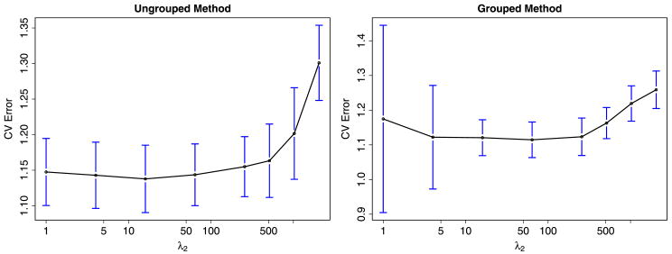
Instead we opted to use a two stage approach. We first computed the “relaxed” cross validated error over a grid of λ₁'s and λ₂'s and selected the tuning parameters corresponding to the minimum. It is well known that cross validation can perform poorly on model selection problems involving L₁ penalties [Meinshausen and Buehlmann (2008)]. This is mainly a result of shrinkage in the coefficient estimates. A common approach to reduce the shrinkage problem in the Lasso involves replacing the nonzero coefficients with their corresponding least squares estimates. Our relaxed cross validation approach works in a similar way. For each combination of λ₁ and λ₂, we first use equations (4) and (5) to identify initial estimates for A and P. We then fix P and the zero elements of A and use “least squares” to estimate the nonzero elements of A. The cross validated errors are then computed based on these “un-shrunk” estimates for A. We have found that this approach allows us to select sparser network structures than those from using standard cross validation. Figure 3 shows the cross validated error rates for different values of λ₂ with λ₁ = 64. For the grouped method the minimum was achieved with λ₁ = λ₂ = 64, while the ungrouped minimum was achieved with λ₁ = 64 and λ₂ = 16.

Fig. 3.

Cross validated error rates as a function of λ₂ for the ungrouped and grouped methods. The blue vertical lines indicate variability in the cross validated error.

Second, we used a parametric bootstrap analysis to determine whether there was significant evidence that an element in A was nonzero. We ran our method on 100 bootstrap samples, each created by first computing the residuals ê = E − Â P̂, resampling ê, and then generating the bootstrap sample E^(b) = Â P̂ + ê^(b). For each element of A, we computed a corresponding p-value based on the 100 bootstrap results, thus, we had approximately 2000 p-values. Since this constituted a significant multiple testing problem, we used False Discovery Rate (FDR) methods to set a cutoff such that the FDR was no more than 0.05. Elements in A with p-values smaller than the cutoff were left as is while the remainder were set to zero. All the results that follow are based on this bootstrap analysis.

4.3. Results

The results from our analysis of the 35 experiments suggested that a significant portion of the potential binding sites should be discarded. Now 18 TFs were expected to regulate 20 or fewer genes and 26 of the 37 TFs were expected to regulate at most 50 genes. Even CRP went from over 500 potential binding sites in the prior to fewer than 500 in the posterior. The posterior estimate for A contained 1766 nonzero entries, approximately a 15% reduction in the number of connections compared to our prior guess for the network. Figure 4 provides graphical representations for the prior and posterior networks. Notice that in the posterior estimate there are many fewer connections and, as a result, there are numerous genes and one TF that are no longer connected to the rest of the network, suggesting there is no evidence that these particular genes are regulated by any of the 37 TFs we examined. The fact that one of the TFs is not connected to the network is likely due to it not being activated in any of the experiments considered, so that there is no detectable correlation in expression among the group of genes that it regulates.

Fig. 4.

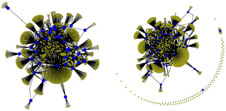
Prior network (left) and posterior estimate produced using the ungrouped method (right). The large blue circles correspond to the 37 transcription factors while the yellow circles represent the 1433 genes. The lines joining blue and yellow circles indicate network connections.

Sabatti and James (2006) discuss several possible reasons for the changes between the initial and final network structure. In brief, Vocabulon works entirely using the sequence information. Hence, it is quite possible for a portion of the E. coli genome sequence to look just like a binding site for a TF, resulting in a high probability as estimated by Vocabulon, when in reality it is not used by the protein in question. In addition, Vocabulon searches for binding sites in the regulatory region of each gene by inspecting 600 base pairs upstream of the start codon which often causes Vocabulon to investigate the same region for multiple genes. If a binding site is located in such a sequence portion, it will be recorded for all of the genes whose “transcription region” covers it.

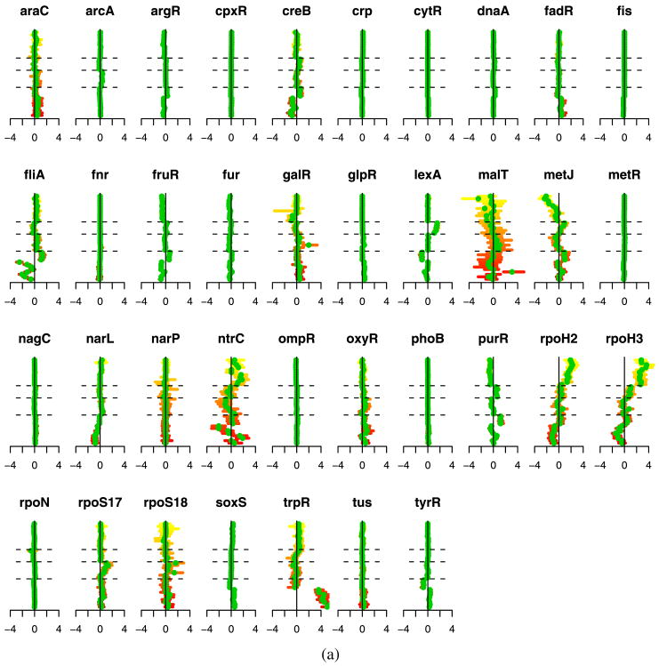
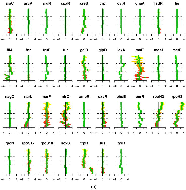
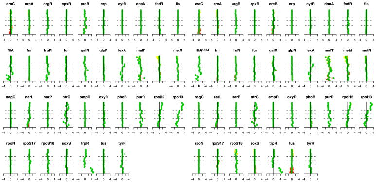
Figure 5 illustrates the estimated transcription factor activation levels using both the ungrouped and grouped methods. We have several ways to validate these results. First, we note that the estimated activation levels show very strong similarities to the results of Sabatti and James (2006). Both their results and ours show the following characteristics. First, there are a number of transcription factors that are not activated in any of the experiments. Focusing on the regulons that are activated in some of the experiments, we note that our method produces results that correspond to the underlying biology. For example, the first 8 experiments [Khodursky et al. (2000)]—represented in the lower portion of the displays from bottom up— are two 4-point time courses of tryptophan starvation. The absence of tryptophan induces the de-repression of the genes regulated by trpR. Correspondingly, our results indicate a clear increase in expression for trpR. In arrays 9–12, the cells were provided with extra tryptophan. Hence, for these experiments we would expect lowered expression. Our results show a negative effect, though the magnitude is small. Additionally, the argR and fliA regulons can be seen to move in the opposite direction to trpR, which corresponds to what has been documented in the literature [Khodursky et al. (2000)].

Fig. 5.

(a) Ungrouped and (b) grouped methods. Each plot corresponds to the experiments for one transcription factor. Experiments are organized along the vertical axis, from bottom to top, with dashed lines separating the experiment groups. Green dots indicate the estimates for p̃_jt and the horizontal bars provide bootstrap confidence intervals.

Experiments 20–24, which correspond to the results between the second and third horizontal dashed lines, are a comparison of wild type E. coli cells with cells that were irradiated with ultraviolet light, which results in DNA damage. Notice that lexA appears to be activated in these experiments, as one would predict since many of the DNA damaged-genes are known to be regularly repressed by lexA [Courcelle et al. (2001)]. Finally, ntrC, purR, rpoH2 and rpoH3 all show activations in the protein overexpression data, the final 11 experiments. In particular, notice that rpoH2 and rpoH3 present the same profile across all experiments. This provides further validation of our procedure since these two really represent the same protein, and are listed separately because they correspond to two different types of binding sites of the TF. Overall, these results conform to the known biology, but also suggest some additional areas for exploration.

The main differences between our results and those of Sabatti and James (2006) are that our penalties on P tend to generate more exact zero estimates than the Bayesian approach, providing somewhat easier interpretation. The grouped and ungrouped results are also similar, but the grouped method tends to produce slightly more sparsity in P, for example, in metJ and rpoS18.

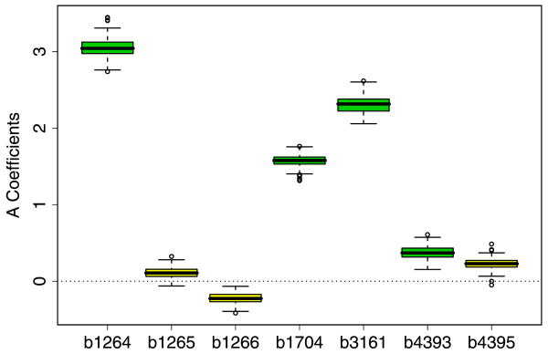
Next, we examine the estimates for A. Since a number of TF's showed no activation in these experiments, we would not expect to be able to accurately estimate their control strengths on the genes. Hence, we will concentrate our analysis here on trpR because this was the most strongly activated TF. Figure 6 presents our estimates of ã for seven genes associated with the trpR. Each boxplot illustrates the 100 bootstrap estimates of ã for a particular gene. The first three boxplots correspond to genes b1264, b1265, b1266. The b-numbers, that identify the genes, roughly correspond to their genomic location, so it is clear that the genes are adjacent to each other. Gene b1264 is known to be regulated by trpR, so it's π_ij was set to 1. The other two genes were chosen by Vocabulon as potential candidates because the binding site for b1264 was also in the search regions for b1265 and b1266, that is, these were cases of the overlapping regulatory regions described previously. While Vocabulon was unable to determine whether a connection existed between b1265, b1266 and trpR, using our approach, we can see that, while ã for b1264 is large, the estimates for b1265 and b1266 are essentially zero. These results show that the expression levels of b1264 correlate well with those of the other genes, but those for b1265 and b1266 do not. Thus, it is possible to use our model to rule out the regulation of two genes by trpR that are within a reasonable distance from a trpR real binding site. Among the remaining four genes, b1704, b3161 and b4393 are all known to be regulated by trpR. Correspondingly, they all have moderate to large estimated activation strengths. b4395 again has an overlapping regulatory region to b4393. The results suggest this is not regulated by trpR.

Fig. 6.

Boxplots of the bootstrap estimates for ã for seven different genes.

4.4. Relaxing zero coefficients

The results from Section 4.3 use the same relatively sparse initial network structure as that of Sabatti and James (2006). Recall the structure we have assumed so far contained only three possible values for π, that is, π_ij = 0, π_ij = 0.5 or π_ij = 1. All connections with π_ij = 0 are forced to remain at zero whatever the gene expression data may suggest. However, as discussed previously, our methodology is able to handle far less sparse structures. Hence, we next investigated the sensitivity of our results to the initial structure by randomly adjusting certain TF-gene connections. In particular, we randomly selected 200 of the connections where π_ij = 0 and reset them to π_ij = 0.5. We also reset all connections where π_ij = 1 to π_ij = 0.5 so that all connections were treated equivalently. We then reran the ungrouped and grouped methods using the new values for π.

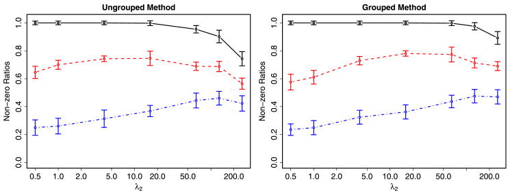
Figure 7 provides plots of the resulting fractions of nonzero estimates for ã_ij, as a function of λ₂ with λ₁ set to 64. A clear pattern emerges with the fraction of nonzeros where there was documented evidence very high (black solid line). Somewhat lower is the fraction of nonzeros for the connections suggested by Vocabulon (red dashed line). Finally, the lowest level of nonzeros is exhibited where there was no significant evidence of a connection (blue dash–dot line). These results are comforting because they suggest that our methodology is able to differentiate between the clear, possible and unlikely connections even when π_ij is equal for all three groups. In addition, there appears to be evidence that the Vocabulon algorithm is doing a good job of separating potential from unlikely connections. Finally, these results illustrate that, unlike the Bayesian approach, it is quite computationally feasible for our methodology to work on relatively dense initial network structures.

Fig. 7.

Fraction of nonzero ã_ij 's as a function of λ₂ for the ungrouped and grouped methods. The black solid line corresponds to those connections where there was documented evidence of a relationship, the red dashed line to where the Vocabulon algorithm suggested there was a relationship and the blue dash–dot line to where there was no evidence of a relationship.

5. Simulation study

After fitting the E. coli data we conducted a simulation study to assess how well our methodology could be expected to reconstruct transcription regulation networks with characteristics similar to those for our data set. We compared our method with two other possible approaches: the penalized matrix decomposition (PMD) method of Witten, Tibshirani and Hastie (2009) and the Bayesian factor analysis model (BFM) of West (2003).

The estimated matrices,  and P̂, and the prior probability estimates, π_ij, from Section 4 were used as the starting point for generating the gene expression levels. In particular, we first let à =  + ε_A, P̃ = P̂ + ε_P, where ε_Aij ∼ S_A ×N(0, σ² (Â)) and ε_Pij ∼ S_P × N (0, σ²(P̂_i)) are noise terms. Depending on the simulation run, S_A was set to either 0.2 or 0.4, while S_P was set to either 0.1 or 0.3. Next, all elements of à corresponding to π_ij = 0 were set to zero. In addition, among elements where π_ij = 0.5, we randomly set ρ of the Ã's to zero where ρ was set to either 60% or 80%. The expression levels were then generated using

$$E=\stackrel{\sim }{A}\stackrel{\sim }{P}+S_N\times \stackrel{\sim }{\Gamma },$$

where Γ̃ is a matrix of error terms with Γ̃_ij ∼ N(0,1) and S_N was set to either 0.2 or 0.4. We produced one simulation run for each combination of S_A, S_P, ρ, and S_N, resulting in a total of 16 simulations.

For each simulation run we generated a new data set, implemented the grouped and ungrouped methods, as well as the PMD method, using different possible tuning parameters to estimate A and P, and computed the corresponding False Positive Rates (FPR) and the True Positive Rates (TPR). The FPR is defined as the fraction of estimated nonzero coefficients, a_ij, among all elements of à where ã_ij = 0 and π_ij = 0.5. The TPR is defined as the fraction of estimated nonzero coefficients, a_ij, among all elements of à where ã_ij ≠ 0 and π_ij = 0.5. The BFM approach turned out to run extremely slowly, taking many hours for just a single tuning parameter. Hence, it was only feasible to implement this method for one set of tuning parameters. For our method, since we have prior information, we can match the columns of the estimated A with the true A in order to compute the sensitivity and specificity etc., but for both PMD and BFM, there is no automatic alignment. In order to ensure a fair comparison, we used a sequential alignment approach to match the columns of the estimated and true A. We first matched each column of the estimated A with each column of the true A and linked the pair that matched best. Then we removed the pair and repeated the process until all columns were aligned.

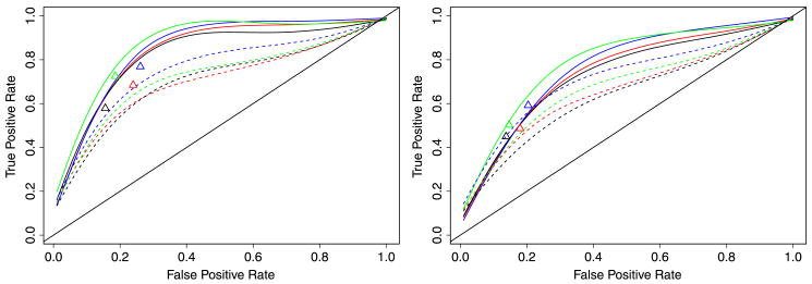
Figure 8 provides a summary of the results from running the ungrouped, PMD and BFM approaches on the eight simulations corresponding to S_P = 0.1. The results from the grouped method and for S_P = 0.3 were similar and hence are not repeated here. Each curve corresponds to the FPR vs TPR for one simulation run using different tuning parameters. The results suggest that our method achieves a reasonable level of accuracy for this data. For example, with S_N = 0.2 we produce an 80% TPR at the expense of a 20% FPR. To lower the FPR to 10% decreases the TPR to approximately 60%. Even with S_N = 0.4, a relatively high noise level, we can achieve a 60% TPR at the expense of a 20% FPR. The PMD method performs relatively worse, for example, producing only a 60% TPR at the expense of a 20% FPR with S_N = 0.2. Assessing BFM is more difficult, given that we were only able to observe its performance at a few points. It appears to outperform PMD and produce results close to our ungrouped method. However, BFM does not seem to be practical on large data sets like our E. coli data given the time required to produce a single fit, without even attempting to select tuning parameters. These results show that indeed there is an advantage to including prior information when available.

Fig. 8.

Simulation results. Solid lines correspond to the ungrouped approach, dashed lines to PMD and triangles to BFM. Red: ρ = 0.6, S_A = 0.2. Black: ρ = 0.8, S_A = 0.2. Blue: ρ = 0.6, S_A = 0.4. Green: ρ = 0.8, S_A = 0.4. Left plot: low noise scenario, S_N = 0.2. Right plot: high noise scenario, S_N = 0.4.

6. Discussion

We have introduced a new methodology for estimating the parameters of model (1) associated with a bipartite network, as illustrated in Figure 1. Our approach is based on introducing L₁ penalties to the regression framework, and using prior information about the network structure.

We have focused on the application of this model to reconstruction of the E. coli transcription network, as this allows easy comparison with previously proposed models. Our approach has the advantage, over the work of Liao et al. (2003) and Sabatti and James (2006), that it does not require assuming prior knowledge of a large fraction of the network. When we utilize the same prior structure as used in Sabatti and James (2006), we get similar, and biologically sensible, results. However, by relaxing the prior assumptions on the sparsity of the network structure, we gain additional insights such as independent validation, both of the experimentally derived network connections and also the connections suggested by the Vocabulon algorithm.

While we tested our methodology on the E. coli data, our approach is potentially applicable to many other organisms, allowing researchers to start to explore many other transcription networks such as those of humans. In particular, there are many organisms for which far less of the TRN structure is known a priori, making it impossible to use the algorithms in Liao et al. (2003) and Sabatti and James (2006). In these cases our L₁ -penalization approach could still be applied provided an “adequate” prior could be generated. For example, in the case of human data, one would probably rely on ChIP chip experiments to provide the back-bone prior data on the possible location of binding sites. Finally, it is worth recalling that, while we describe how to set the π values with specific reference to TRN, the L₁ -penalized regression approach can be used to estimate parameters of bipartite networks arising in other scientific contexts.

Appendix: Identifiability

Liao et al. (2003) provide the following sufficient conditions for identifiability of the transcription regulation network model (1):

1. The connectivity matrix, A, must have full-column rank.

2. When a node in the regulatory layer is removed along with all of the output nodes connected to it, the resulting network must be characterized by a connectivity matrix that still has full-column rank. This condition implies that each column of A must have at least L − 1 zeros.

3. P must have full row rank. In other words, each regulatory signal cannot be expressed as a linear combination of the other regulatory signals.

In our case these conditions were not satisfied because L > T so P was not of full rank. However, the prior was very sparse with many zero elements and relatively few values close to one, so it seemed reasonable to assume that the model was identifiable. To ensure this was correct, we ran our fitting procedure 200 times on the E. coli data, using randomized starting values, and examined the resulting estimates for P. Figure A.1 plots the best 20 (left) and worst 20 results (right), in terms of the final objective values. There are some minor differences in the estimates, but overall the results are encouragingly similar. This experiment provided two useful pieces of information. First, it strongly suggested that, at least for our prior, there were no identifiability problems. Second, it also implied that the fitting algorithm was not getting stuck in any local minima's and was reaching a global optimum.

Fig. A.1.

Left: Best 20 runs. Right: Worst 20 runs.

References

- Alter O, Brown P, Botstein D. Singular value decomposition for genome-wide expression data processing and modeling. Proc Natl Acad Sci. 2000;97:10101–10106. doi: 10.1073/pnas.97.18.10101. [DOI] [PMC free article] [PubMed] [Google Scholar]
- Anderson T. An Introduction to Multivariate Statistical Analysis. Wiley; New York: 1984. MR0771294. [Google Scholar]
- Beal M, Falciani F, Ghahramani Z, Rangel C, Wild D. A Bayesian approach to reconstructing genetic regulatory networks with hidden factors. Bioinformatics. 2005;21:349–356. doi: 10.1093/bioinformatics/bti014. [DOI] [PubMed] [Google Scholar]
- Boulesteix A, Strimmer K. Predicting transcription factor activities from combined analysis of microarray and chip data: A partial least squares approach. Theor Biol Med Model. 2005;2:23. doi: 10.1186/1742-4682-2-23. [DOI] [PMC free article] [PubMed] [Google Scholar]
- Brynildsen M, Tran L, Liao J. A Gibbs sampler for the identification of gene expression and network connectivity consistency. Bioinformatics. 2006;22:3040–3046. doi: 10.1093/bioinformatics/btl541. [DOI] [PubMed] [Google Scholar]
- Candes E, Tao T. The Dantzig selector: Statistical estimation when p is much larger than n (with discussion) Ann Statist. 2007;35:2313–2351. MR2382644. [Google Scholar]
- Chang C, Ding Z, Hung Y, Fung P. Fast network component analysis (fastNCA) for gene regulatory network reconstruction from microarray data. Bioinformatics. 2008;24:1349–1358. doi: 10.1093/bioinformatics/btn131. [DOI] [PubMed] [Google Scholar]
- Courcelle J, Khodursky A, Peter B, Brown PO, Hanawalt PC. Comparative gene expression profiles following UV exposure in wild-type and SOS-deficient Escherichia coli. Genetics. 2001;158:41–64. doi: 10.1093/genetics/158.1.41. [DOI] [PMC free article] [PubMed] [Google Scholar]
- Efron B, Hastie T, Johnston I, Tibshirani R. Least angle regression (with discussion) Ann Statist. 2004;32:407–451. MR2060166. [Google Scholar]
- Fan J, Li R. Variable selection via nonconcave penalized likelihood and its oracle properties. J Amer Statist Assoc. 2001;96:1348–1360. MR1946581. [Google Scholar]
- Friedman J, Hastie T, Hofling H, Tibshirani R. Pathwise coordinate optimization. Ann Appl Statist. 2007;1:302–332. MR2415737. [Google Scholar]
- Fu W. Penalized regressions: The Bridge versus the Lasso. J Comput Graph Statist. 1998;7:397–416. MR1646710. [Google Scholar]
- James GM, Radchenko P. A generalized Dantzig selector with shrinkage tuning. Biometrika. 2009;96:323–337. [Google Scholar]
- Khodursky AB, Peter BJ, Cozzarelli NR, Botstein D, Brown PO, Yanofsky C. DNA microarray analysis of gene expression in response to physiological and genetic changes that affect tryptophan metabolism in Escherichia coli. Proc Natl Acad Sci USA. 2000;97:12170–12175. doi: 10.1073/pnas.220414297. [DOI] [PMC free article] [PubMed] [Google Scholar]
- Lee DD, Seung HS. Learning the parts of objects by non-negative matrix factorization. Nature. 1999;401:788–793. doi: 10.1038/44565. [DOI] [PubMed] [Google Scholar]
- Lee DD, Seung HS. Algorithms for non-negative matrix factorization. Advances in Neural Information Processing Systems. 2001;13:556–562. [Google Scholar]
- Lee S, Batzoglou S. Application of independent component analysis to microarrays. Genome Biol. 2003;4:76. doi: 10.1186/gb-2003-4-11-r76. [DOI] [PMC free article] [PubMed] [Google Scholar]
- Li Z, Shaw S, Yedwabnick M, Chan C. Using a state-space model with hidden variables to infer transcription factor activities. Bioinformatics. 2006;22:747–754. doi: 10.1093/bioinformatics/btk034. [DOI] [PubMed] [Google Scholar]
- Liao JC, Boscolo R, Yang Y, Tran L, Sabatti C, Roychowdhury V. Network component analysis: Reconstruction of regulatory signals in biological systems. Proc Natl Acad Sci. 2003;100:15522–15527. doi: 10.1073/pnas.2136632100. [DOI] [PMC free article] [PubMed] [Google Scholar]
- Meinshausen N. Relaxed Lasso. Comput Statist Data Anal. 2007;52:374–393. MR2409990. [Google Scholar]
- Meinshausen N, Buehlmann P. Stability selection. J Roy Stat Soc Ser B. 2008 To appear. Available at arXiv:0809.2932v1.
- Oh MK, Liao JC. DNA microarray detection of metabolic responses to protein overproduction in Escherichia coli. Metabolic Engineering. 2000a;2:201–209. doi: 10.1006/mben.2000.0149. [DOI] [PubMed] [Google Scholar]
- Oh MK, Liao JC. Gene expression profiling by dna microarrays and metabolic fluxes in Escherichia coli. Biotechnol Prog. 2000b;16:278–286. doi: 10.1021/bp000002n. [DOI] [PubMed] [Google Scholar]
- Oh MK, Rohlin L, Liao JC. Global expression profiling of acetate-grown Escherichia coli. J Biol Chem. 2002;277:13175–13183. doi: 10.1074/jbc.M110809200. [DOI] [PubMed] [Google Scholar]
- Pournara I, Wernisch L. Factor analysis for gene regulatory networks and transcription factor activity profiles. BMC Bioinformatics. 2007;8 doi: 10.1186/1471-2105-8-61. [DOI] [PMC free article] [PubMed] [Google Scholar]
- Radchenko P, James GM. Variable inclusion and shrinkage algorithms. J Amer Statist Assoc. 2008;103:1304–1315. MR2462899. [Google Scholar]
- Sabatti C, James GM. Bayesian sparse hidden components analysis for transcription regulation networks. Bioinformatics. 2006;22:737–744. doi: 10.1093/bioinformatics/btk017. [DOI] [PubMed] [Google Scholar]
- Sabatti C, Lange K. Genomewise motif identification using a dictionary model. IEEE Proceedings. 2002;90:1803–1810. [Google Scholar]
- Sanguinetti G, Lawrence N, Rattray M. Probabilistic inference of transcription factor concentrations and gene-specific regulatory activities. Bioinformatics. 2006;22:2775–2781. doi: 10.1093/bioinformatics/btl473. [DOI] [PubMed] [Google Scholar]
- Sun N, Carroll R, Zhao H. Bayesian error analysis model for reconstructing transcriptional regulatory networks. Proc Natl Acad Sci. 2006;103:7988–7993. doi: 10.1073/pnas.0600164103. [DOI] [PMC free article] [PubMed] [Google Scholar]
- Tibshirani R. Regression shrinkage and selection via the Lasso. J Roy Statist Soc Ser B. 1996;58:267–288. MR1379242. [Google Scholar]
- Tran L, Brynildsen M, Kao K, Suen J, Liao J. gNCA: A framework for determining transcription factor activity based on transcriptome: Identifiability and numerical implementation. Metab Eng. 2005;7:128–141. doi: 10.1016/j.ymben.2004.12.001. [DOI] [PubMed] [Google Scholar]
- West M. Bayesian factor regression models in the “large p, n” paradigm. Bayesian Statist. 2003;7:733–742. MR2003537. [Google Scholar]
- Witten DM, Tibshirani R, Hastie T. A penalized matrix decomposition, with applications to sparse principal components and canonical correlation analysis. Biostatistics. 2009;10:515–534. doi: 10.1093/biostatistics/kxp008. [DOI] [PMC free article] [PubMed] [Google Scholar]
- Yu T, Li K. Inference of transcriptional regulatory network by two-stage constrained space factor analysis. Bioinformatics. 2005;21:4033–4038. doi: 10.1093/bioinformatics/bti656. [DOI] [PubMed] [Google Scholar]
- Zou H. The adaptive Lasso and its oracle properties. J Amer Statist Assoc. 2006;101:1418–1429. MR2279469. [Google Scholar]
- Zou H, Hastie T. Regularization and variable selection via the elastic net. J Roy Statist Soc Ser B. 2005;67:301–320. MR2137327. [Google Scholar]