Image Atlas Construction via Intrinsic Averaging on the Manifold of Images

Abstract

In this paper, we propose a novel algorithm for computing an atlas from a collection of images. In the literature, atlases have almost always been computed as some types of means such as the straightforward Euclidean means or the more general Karcher means on Riemannian manifolds. In the context of images, the paper’s main contribution is a geometric framework for computing image atlases through a two-step process: the localization of mean and the realization of it as an image. In the localization step, a few nearest neighbors of the mean among the input images are determined, and the realization step then proceeds to reconstruct the atlas image using these neighbors. Decoupling the localization step from the realization step provides the flexibility that allows us to formulate a general algorithm for computing image atlas. More specifically, we assume the input images belong to some smooth manifold M modulo image rotations. We use a graph structure to represent the manifold, and for the localization step, we formulate a convex optimization problem in ℝ^k (k the number of input images) to determine the crucial neighbors that are used in the realization step to form the atlas image. The algorithm is both unbiased and rotation-invariant. We have evaluated the algorithm using synthetic and real images. In particular, experimental results demonstrate that the atlases computed using the proposed algorithm preserve important image features and generally enjoy better image quality in comparison with atlases computed using existing methods.

1. Introduction

Computing an atlas from a collection of images is a fundamental problem in medical imaging and computer vision. (e.g., [10, 7, 6, 21]). Since the atlas is supposed to be an informative representative of the given set of images, in most existing approaches, the atlas construction problem is often formulated as some kind of mean estimation problem. For example, one of the popular existing methods for computing an atlas is the unbiased diffeomorphic atlas construction algorithm proposed in [7]. If {I₁, · · ·, I_k} denote the input images, [7] solves the atlas construction problem using a variational approach based on the large deformation diffeomorphism framework described in [12, 3, 13]. The image atlas I is given as:

$$\mathbf{I}\equiv \underset{\stackrel{\sim }{\mathbf{I}}\in \mathcal{I}}{\text{argmin}}\sum _{i=1}^k{\mathbf{d}}_{\mathcal{I}}^2({\mathbf{I}}_i,\stackrel{\sim }{\mathbf{I}}),$$ (1)

where is a metric on the space of images. Geometrically, Equation 1 can be interpreted as computing the mean of the collection of points (images) {I₁, · · ·, I_k} in the metric space (, ).

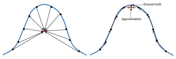
Figure 1 shows the result of applying the above method to a collection of 2D images. The result is clearly unsatisfactory in that the atlas image is blurry and many important details are missing or are corrupted. A geometric explanation for this result is offered in Figure 2: The smooth variation of the images allows us to assume that these images belong to some smooth submanifold M in . [7] computes the mean of the images in the ambient space , and as the figure shows, there is no guarantee that the result will be on M. Clearly, the correct mean in this case should be the mean of the images considered as the points on M. Based on the seminal paper of Karcher [9], numerical computation of means on Riemannian manifolds has received considerable attention in the past few years (e.g., [20, 14]), and there is already a body of recent works that applies these techniques to vision problems (e.g., [5, 22]). Unfortunately, all of these methods require the precise knowledge of the Riemannian metric, and this limits the current techniques to mostly symmetric Riemannian manifolds, examples of which include the Grassmanians and the symmetric positive-definite matrices, etc.. In our case, the manifold M and its metric are both unknown. Therefore, we need a method that can estimate the mean on M without using the metric on M, a requirement that seems contradictory at first. However, Figure 2 also reveals one thing that is often valid in that the mean on M can be approximated well by, for example, averaging a few of its neighbors. The challenge here is, of course, to identify these neighbors in M without knowing explicitly the Riemannian structure of M. In particular, this also suggests that in the context of working with images, computing image atlases should be a two-step process: localize the mean first by determining these neighbors and realize this abstract mean as the atlas image using these neighbors. The two steps are qualitatively different in that the localization step utilizes the entire set of input images. It uses the global geometry to determine these crucial neighbors among the input images, and the realization step that follows uses only these neighbors for constructing the image.

Figure 1.

Left: Images of an object. Center: The atlas computed using [7]. Right: The atlas computed using the proposed algorithm.

Figure 2.

Ten points on an one-dimensional manifold. Left Mean for the ten points computed using the metric of the ambient space. Right Mean computed using the metric of the submanifold M. Note that the mean can be approximated by using just two points on M, the two points that are closest to the mean on M.

In many applications, it is reasonable to demand rotation invariance for the atlas, and Figure 3 shows one example. More specifically, suppose I is the atlas for {I₁, · · ·, I_k} and if k different rotations g_i are applied to these images to form a new collection {g₁(I₁), · · ·, g_k(I_k)}, then the atlas Ĩ for the latter collection should be related to I by some rotation. This requirement is desirable because the image contents of I_i and g_i(I_i) are essentially the same, and modulo the rotations, these two image collections are completely equivalent. Therefore, it is reasonable to require that their atlases are also equivalent modulo rotations, i.e., Ĩ = g(I) for some rotation g. However, this requirement means that we can no longer assume that the input images belong to some submanifold M in . Instead, the correct assumption should be that modulo rotations, the images belong to a submanifold M in the quotient space Q of [17, 16].

Figure 3.

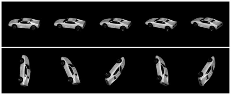
Top Row Images of a car. The smooth variation of the images allows the assumption that these images belong to a smooth submanifold M in . Bottom Row Rotations are applied to the images in the row above. The appearance variation in this collection is erratic, and it is difficult to assume that they belong to a smooth submanifold in .

In this paper, we propose a novel approach to the atlas construction problem that incorporates the ideas discussed above. Starting with a rotation-invariant metric on , it induces a metric d_Q on the quotient space Q. The proposed algorithm computes the atlas as an approximation of the mean m of the images considered as points on M. In general, the metric on M is unknown; however, the pairwise geodesic distances m_ij = d_M(I_i, I_j) between images can be estimated using the metric in Q [8]. An important element in the proposed algorithm is to estimate the geodesic distances d_M(m, I_i) between the mean m and images I_i using the pairwise geodesic distances m_ij as the inputs. We formulate this as a convex optimization problem in IR^k, and the solution to this optimization problem will provide an approximations to d_M(m, I_i). This will allow us to locate the mean m on the manifold M and identify images that are neighbors of m (belonging to a neighborhood of m). These neighbors (images) are used, together with their geodesic distances d_M(m, I_i) to the mean, to form the image for m, which, before this point, is simply an abstract point in M. It is straightforward to show that the proposed algorithm is both unbiased and rotation-invariant. Preliminary experimental results have shown that, with greater preservation of important image features and details, the image atlases produced by the proposed algorithm enjoy better image quality when compared with atlases obtained using exiting methods.

The rest of this paper is organized as follows: in Section 2, we describe the theoretical framework for image atlas construction. Experimental results for synthetic and real image data are presented in Section 3. Finally, we conclude in section 4.

2. A Theoretical Framework for Atlas Construction

In the following discussion, will denote the space of images. Images in are defined formally as L²-functions on a finite domain Ω ⊂ IRⁿ, where Ω is the underlying coordinate system for the images in (n = 2 for 2D images and n = 3 for 3D images). Let ≡ {I₁, · · ·, I_k} denote a collection of k images and g(I)(x) = I(g⁻¹(x)) for g ∈ SO(n) and x ∈ Ω. In this section, we will define the image atlas I for the image collection and outline an algorithm for computing I. We require the algorithm to satisfy the following two properties:

1. Unbiasedness: The algorithm output should not depend on the particular ordering of the images in the collection .

2. Rotation Invariance: If ${\mathcal{C}}^{\prime }\equiv \{{\mathbf{I}}_1^{\prime },\cdots ,{\mathbf{I}}_k^{\prime }\}$ are images obtained by applying k rotations to images in : ${\mathbf{I}}_i^{\prime }=g_i({\mathbf{I}}_i)$ for g_i ∈ SO(n), 1 ≤ i ≤ k, then the atlas I′ for the image collection is related to I by a rotation g ∈ SO(n): I′ = g(I).

2.1. Geometry of the Quotient Space Q

The demand for rotation invariance requires us to work not in but in Q, the quotient space of by the rotation SO(n) (see [17, 16] for details). Basically, Q is a space that parameterizes the SO(n)-orbits in and in this paper, we will assume that Q has a manifold structure induced from the manifold structure of . Let π : → Q denote the canonical projection map that sends each image I ∈ to the unique SO(n)-orbit [I] ∈ Q containing I: π(I) = [I]. The points {[I₁], · · ·, [I_k]} are assumed to belong to a smooth submanifold M in Q. As a submanifold of Q, M is equipped with the natural induced Riemannian metric and we let d_M([I_i], [I_j]) denote the geodesic distance function on M. Let m denote the mean of {[I₁], · · ·, [I_k]} with respect to d_M, and the atlas [I] computed by our algorithm will be a suitable approximation of m.

SO(n)-invariant metric is defined as

$${\mathbf{d}}_{\mathcal{I}}({\mathbf{I}}_1,{\mathbf{I}}_2)={\mathbf{d}}_{\mathcal{I}}(g({\mathbf{I}}_1),g({\mathbf{I}}_2)),$$

for any two images I₁, I₂ ∈ and g ∈ SO(n). Many metrics can be easily shown to be SO(n)-invariant, such as L²-metric and the following metric defined in [2]:

$${\mathbf{d}}_{\mathcal{I}}({\mathbf{I}}_1,{\mathbf{I}}_2)=\underset{h_i}{min}{\left({\int }_{\mathrm{\Omega }}{\mid {\mathbf{I}}_1(h_i(x))-{\mathbf{I}}_2\mid }^{2}dx+{\int }_0^1{\int }_{\mathrm{\Omega }}{\left|\right|{Lv}_i\left|\right|}^2\mathit{dxds}\right)}^{1/2}$$ (2)

where v_i is the time-dependent vector field that defines the diffeomorphic flow from the identity to the diffeomorphism h_i, and L is a second-order elliptic operator. Any SO(n)-invariant metric on induces a metric d_Q in Q using the formula [16]

$${\mathbf{d}}_{\mathbf{Q}}([x],[y])=\underset{s\in [x],t\in [y]}{min}{\mathbf{d}}_{\mathcal{I}}(s,t)$$ (3)

for any two points [x], [y] ∈ Q¹. The two related metrics , d_Q allows us to go between and Q. For example, computing the mean in Q minimizes the following function,

$$[\mathbf{I}]=\underset{[{\mathbf{I}}^{\prime }]\in \mathbf{Q}}{\text{argmin}}\sum _{i=1}^k{\mathbf{d}}_{\mathbf{Q}}^2([{\mathbf{I}}_i],[{\mathbf{I}}^{\prime }]).$$

The corresponding function to minimize in would be (using Equation 3)

$$\mathbf{I}=\underset{{\mathbf{I}}^{\prime }\in \mathcal{I},s_1,\cdots ,s_k\in \mathbf{SO}(n)}{\text{argmin}}\sum _{i=1}^k{\mathbf{d}}_{\mathcal{I}}^2(s_i({\mathbf{I}}_i),{\mathbf{I}}^{\prime }).$$

In particular, we have ρ(I) = [I] and I ∈ π⁻¹([I]). Following the similar approach in Isomap [8], we could compute pair-wise geodesic distance d_M([I_i], [I_j]) using the induced metric d_Q.

2.2. Estimating Mean from Pairwise Geodesic Distances

Suppose {x₁, · · ·, x_k} are points on a manifold M with d_M denoting the Riemannian geodesic distance. One possible way to determine the mean m of x_i on M is the following. Let a_i = d_M(x_i, m), 1 ≤ i ≤ k. Determining a_i is of course equivalent to locating m on M, and a_i can be determined as the solution to an optimization problem given by:

$$\begin{array}{l}min{a}_1^2+a_2^2+\cdots +a_k^2\\ \text{constraints}{a}_i\ge 0,i=1,\cdots k\\ a_i+a_j\ge m_{ij},\\ a_i+m_{ij}\ge a_j,\\ a_j+m_{ij}\ge a_i,i,j=1,\cdots k\\ {\text{HDC}}_{\mathbf{M}}(a_i,m_{ij}),\end{array}$$ (4)

where m_ij = d_M(x_i, x_j) and HDC_M(a_i, m_ij) denote the remaining higher-degree constraints among a_i, m_ij. The collection of constraints in HDC_M depends on M as a metric space and in general, for two different manifolds, their corresponding HDC will be different. The linear inequality constraints between a_i and m_ij are imposed because d_M satisfies the triangle inequality.

For our problem, the manifold M and its metric d_M are unknown, and consequently, the constraints in HDC_M cannot be known. However, as an approximation, we can try to solve the following optimization problem in IR^k and use the solution a₁, · · ·, a_k as an approximation to the solution of the above problem:

$$\begin{array}{l}min{a}_1^2+a_2^2+\cdots +a_k^2\\ \text{constraints}{a}_i\ge 0,i=1,\cdots k\\ a_i+a_j\ge m_{ij},\\ a_i+m_{ij}\ge a_j,\\ a_j+m_{ij}\ge a_i,i,j=1,\cdots k\end{array}$$ (5)

The optimization problem is clearly convex since the objective function is strictly convex (the Hessian is positive-definite everywhere) and the domain, which is the intersection of half-spaces, is also convex. This particular type of optimization problem (with quadratic cost function and linear inequality constraints) can be solved efficiently even with a large number of variables and constraints. And because the object function is strictly convex, the solution is unique [1]. Furthermore, the solution is stable with respect to the input parameters m_ij in the sense that small perturbations of m_ij will not significantly change the solution a₁, · · ·, a_k [1]. For computing robust L¹-median [4] instead of mean, we simply need to change the cost function to a₁ + a₂ + · · · + a_k.

2.3. Computing the Image Atlas I

The non-negative number a_i provides an estimate on the geodesic distance d_M(m, [I_i]). The last step is to use a_i to determine a small number of points in {[I₁], · · ·, [I_k]} that are close to m as measured by d_M, and m is then approximated from these points with respect to the metric d_Q in Q. In practice, a positive integer K is specified and K points [I_i1], · · ·, [I_iK] with shortest distances to m are chosen. We require that K ≥ 1+ dimension of the manifold.

We could approximate m with a weighted mean of the K points [I_ij], with weights w_j, 1 ≤ j ≤ K:

$$[\mathbf{I}]=\underset{[{\mathbf{I}}^{\prime }]\in \mathbf{Q}}{\text{argmin}}\sum _{j=1}^K{w}_j{\mathbf{d}}_{\mathbf{Q}}^2([{\mathbf{I}}_{i_j}],[{\mathbf{I}}^{\prime }])$$

Since a point closer to m contributes more in atlas realization, the weights w_j can be constructed from the estimated geodesic distances a_ij:

$$w_j=b_j/\left(\sum _{k=1}^K{b}_k\right)$$

where $b_j=exp(-a_{i_j}^2/{\sigma }^2)$, 1 ≤ j ≤ K, for some σ > 0. Using the metric defined by Equation 2, the corresponding atlas I is computed by solving the variational problem

$$\underset{\stackrel{\sim }{\mathbf{I}},h_j,s_j}{min}\sum _{j=1}^K{w}_j{\int }_{\mathrm{\Omega }}{\mid {\mathbf{I}}_{i_j}(h_j{s}_j(x))-\stackrel{\sim }{\mathbf{I}}\mid }^{2}dx+{\int }_0^1{\int }_{\mathrm{\Omega }}{\left|\right|{Lv}_j\left|\right|}^2\mathit{dxds}$$ (6)

3. Experiments

In this section, we present three sets of experimental results that evaluate the proposed atlas construction algorithm. In these experiments, we will use both synthetic and real image data, and comparisons will be made with atlases computed using existing methods [4, 7, 21] that are based on non-rigid group-wise registrations.

3.1. Experimental Results Using COIL-20

In the first set of experiments, we compute the image atlas using images from the Columbia Object Image Library dataset (COIL-20) [18]. COIL-20 contains twenty objects, and images for each object are obtained by placing the object on a turntable and rotating it in five-degree increments in front of a fixed camera. This gives 72 images for each object. As the viewpoint varies on a circle, the appearance variation of the images can be modelled using an one-dimensional submanifold M in the image space. In particular, the dataset has been used frequently to evaluate recognition and manifold learning algorithms (e.g., [19]). In this experiment, the number of nearest neighbors K is set to four, and the image atlases for five objects in COIL-20 are shown in Figure 4.

Figure 4.

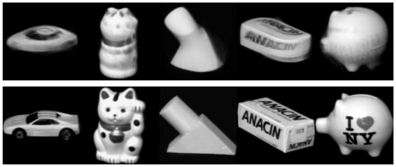
Image atlases for five objects from COIL-20. The images in the first row are the atlases computed using [7]. Our results are shown in the second row.

We validate the algorithm using a known ground truth. Taking the ‘duck’ object in COIL-20, we choose 36 images with pose (viewing angle) ranging from 5° to 90° and −5° to −90°. Several sample images are shown in Figure 5. As the viewpoint varies from −90° to 90°, the manifold M underlies the 36 images has the topology of a semi-circle, and the mean in M can be taken to be the image with 0-degree pose.

Figure 5.

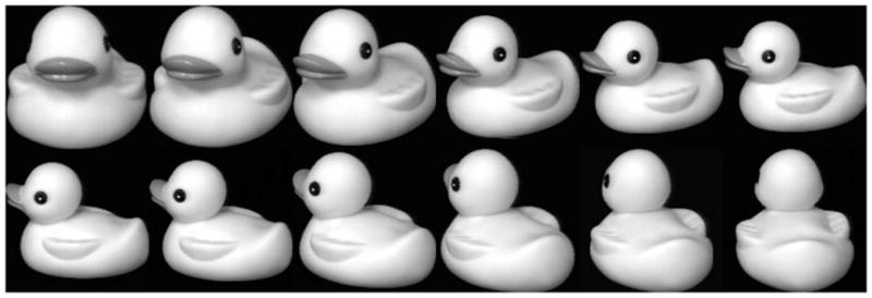
Samples of input duck images.

Figure 6 displays the image atlases (as L²-mean and L¹-median) computed using our method and the algorithms proposed in [7, 4] that use non-rigid group-wise registration. The algorithm in [7] computes the atlases as the L²-mean while [4] constructs the atlases using L¹-median. In both cases, it is clear that our results are much closer to the ground truth than the atlases produced by the other methods. It is not surprising since the two existing methods does not respect the manifold structure and they in fact compute the atlases as the mean and median of the ambient space. Therefore, their images are typically blurry with substantial loss of image details.

Figure 6.

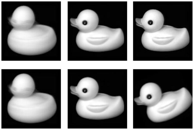
First Row: L ²-mean images obtained using [7] (left) and our algorithm (middle). The image on the right is the ground truth. Second Row: L¹-median images obtained using [4] (left) and our algorithm (middle). The right image is the atlas obtained by our algorithm using the same set of images that are randomly rotated between 20° and 30°.

Finally, we test the rotational invariance of the proposed algorithm. Given the 36 images used to compute the duck atlas above, we randomly rotate these images with angle between 20° and 30°. Since the algorithm factored out the rotations by working in the quotient space, the new and the old atlases should be the same point in the quotient space. That is, they should differ only by a planar rotation. As shown in Figure 6 (Second Row), this is indeed the case.

3.2. Experimental Results Using Synthetic Images

In the second experiment, we synthetically generate 56 images from the Stanford bunny mesh model. The model is centered at the origin and we sample 56 camera locations on the viewing sphere surrounding the model. These 56 locations are uniformly sampled with respect to a central (apex) location ([0 0 1]), with maximum angular deviation from the apex of 30 degrees. These points are plotted in Figure 8. In all the renderings, we assume simple Lambertian reflectance model with the distant lighting direction parallel to the viewpoint (camera location). The 56 images are considered as a collection of sampled points from a two-dimensional submanifold in the image space, and we choose a value of 5 for the parameter K in this experiment. Figure 7 shows the atlas constructed by our method and the two comparisons that use straightforward averaging of intensity values and the unbiased diffeomorphic atlas [7]. Note that outputs from the two competing methods are not satisfactory as many details and features are lost or smoothed out. The camera locations corresponding to the five neighbors (K = 5) closest to the mean determined by our algorithm are shown by the five red points in Figure 8. For this example, it is evident that these five points are near the expected mean for this collection of points on the sphere. Correspondingly, our algorithm produces the image atlas using only images taken from these five viewpoints.

Figure 8.

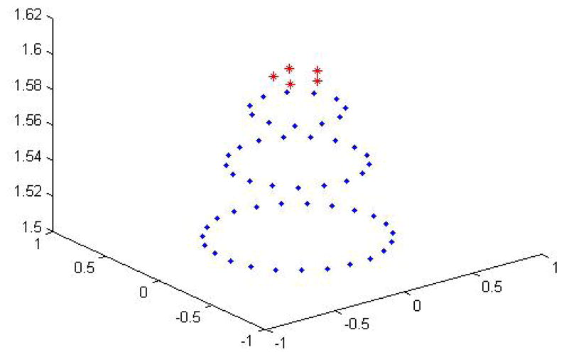
56 Camera locations sampled on the viewing sphere. The camera locations of the five nearest neighbors to the mean determined by our method are shown by the red points.

Figure 7.

Left to right straightforward averaging, unbiased diffeomorphic atlas and our atlas.

3.3. Experimental Results Using OASIS

In the third experiment, we apply the proposed algorithm to construct atlases from collections of MRI images. Specifically, the image data used in the experiment are the MRI images from the freely available Open Access Series of Imaging Studies (OASIS) [11]. OASIS contains MRI brain images from a cross-sectional population of 416 subjects. Each brain image has a resolution of 176×208×176 voxels. The ages of the subjects range from 18 to 96, and it is known that the structural difference in the brain across different age groups can be significant [15]. Therefore, we divide the 416 subjects from OASIS dataset into three groups: youth group (subjects younger than 40), middle-aged group (between 40 and 60) and elderly group (older than 60), and one atlas is computed for each age group. Figure 10 displays sample images from the three age groups, and the computed atlases (using K = 12 nearest neighbors) are shown in Figure 9. For comparison, we use the EM-based iCluster algorithm proposed in [21]. iCluster can automatically cluster a set of images and compute the atlas (template) for each cluster. Applied to the OASIS dataset [21], iCluster clusters the images into three clusters, which differ slightly from the three age groups defined above. However, the two atlases visually look similar and comparable, especially for the youth group since the composition of the youth group in [21] includes 201 subjects (aged 31.2 ± 14.5 years), which is very similar to ours. As shown in Figure 9, the atlases computed by our method are substantially sharper with more structural details. Again, this is not surprising because our atlases are computed as means on the manifolds, instead of the means in the ambient space. Thus, the atlases computed by our method retain important brain structures and they genuinely look like real brains when compared with the real samples in Figure 10. In particular, our method keeps these structures mostly intact and clear while other existing methods (e.g., [21, 7]) blur them to various degrees. For applications such as atlas-based segmentation and registration, prominent structures such as the ventricles are potentially very useful, and therefore, our atlases with more contrasting details should provide better templates for these applications.

Figure 10.

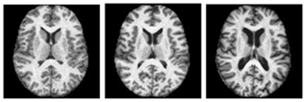
Sample images from from the three age groups. From left to right: youth, middle-aged and elderly.

Figure 9.

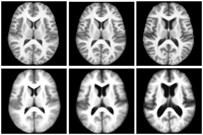
Axial views of atlases. Top Row: Atlases generated using our method for youth, middle-aged and elderly groups (from left to right). Bottom Row: Youth, older middle-aged and elderly templates generated by iCluster [21]. The images shown here are taken directly from [21].

To model the variation within each age group with respect to the atlas, we can use a field of spherical functions that encodes the point-wise deformation. More specifically, we use pairwise nonrigid registration to align each subject in a given age group to its atlas. For each voxel (point) x, these registrations provide a set of displacement vectors v₁, · · ·, v_n that characterizes the local variation relative to the atlas at x. These displacement vectors can then be interpolated using a non-negative spherical function f : S² → ℝ. This results in a field of non-negative spherical functions, and together with the atlas, they provide an effective characterization of the variation in MRI brain images within a given population group. Figure 11 displays a visualization of the field of non-negative spherical functions using a method similar to [23]. Each spherical function is computed from 195 local displacement vectors, and its graph on the sphere is plotted at each point.

Figure 11.

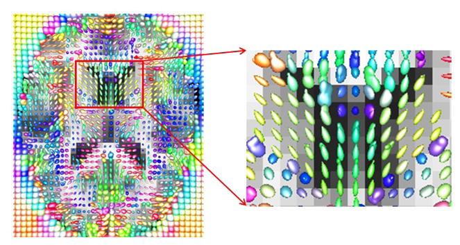
Left: Visualization of the field of non-negative spherical functions. The atlas is from the elderly group with 195 subjects. The spherical functions are represented by their graphs on the sphere: the value f(u) at u ∈ S² gives the height of f at the point u, and the resulting height surface over the sphere is shown. Right: A close-up view of the field.

4. Conclusion

We have proposed a novel approach to the atlas construction problem, an important problem in medical imaging as well as computer vision. We assume that modulo image rotations, the input images I₁, · · ·, I_k belong to a smooth manifold M, and the atlas computed by the proposed algorithm in principle can be considered as an approximation of the mean of I₁, · · ·, I_k with respect to the metric on M. We proposed a two-step algorithm that first locates the mean among the input images and then realizes the atlas image using a few of its neighbors. We have provided several experimental results that validate the proposed algorithm, and in particular, comparisons with existing methods have shown that the atlases computed using our algorithm enjoy better image quality with preservation of important image features and details.

References

- 1.Boyd A, Vandenberghe L. Convex Optimization. Cambridge University Press; 2004. [Google Scholar]
- 2.Davis B, Fletcher P, Bullitt E, Joshi S. Population shape regression from random design data. IEEE International Conference on Computer Vision (ICCV) 2007 [Google Scholar]
- 3.Dupuis P, Grenander U. Variational problems on flows of diffeomorphisms for image matching. Quarterly of applied Mathematics. 1998;2:587–600. [Google Scholar]
- 4.Fletcher P, Venkatasubramanian S, Joshi S. Robust statistics on riemannian manifold via the geometric median. IEEE Conference on Computer Vision and Pattern Recognition (CVPR) 2008 [Google Scholar]
- 5.Goh A, Vidal R. Clustering and dimensionality reduction on riemannain manifolds. Proc IEEE Conf on Comp Vision and Patt Recog. 2008 [Google Scholar]
- 6.Guimond A, Meunier F, Thirion J. Technical Report, 3731, INRIA. 1999. Average brain models: A convergence study. [Google Scholar]
- 7.Joshi S, Davis B, Jomier M, Gerig G. Unbiased diffeomorphic atlas construction for computational anatomy. NeuroImage. 2004;23:S151–S160. doi: 10.1016/j.neuroimage.2004.07.068. [DOI] [PubMed] [Google Scholar]
- 8.Tenenbaum J, de Silva V, Langford J. A global geometric framework for nonlinear dimensionality reduction. Science. 2000;290(5500):2319–2323. doi: 10.1126/science.290.5500.2319. [DOI] [PubMed] [Google Scholar]
- 9.Karcher H. Riemannian centers of mass and mollifier smoothing. Comm on Pure and Appl Math. 1977;30:509–541. [Google Scholar]
- 10.Lorenzen P, Prastawa M, Davis B, Gerig G, Bullitt E, Joshi S. Multi-modal image set registration and atlas formation. Medical Image Analysis MEDIA. 2006;10(3):440–451. doi: 10.1016/j.media.2005.03.002. [DOI] [PMC free article] [PubMed] [Google Scholar]
- 11.Marcus D, Wang T, Parker J, Gsernansky J, Morris J, Buckner R. Open access series of imaging studies (oasis): Cross-section mri data in young, middle aged, nondemented, and demented older adults. Journal of Cognitive Neuroscience. 2007;19:1498–1507. doi: 10.1162/jocn.2007.19.9.1498. [DOI] [PubMed] [Google Scholar]
- 12.Miller M, Younes L. Group actions, homeomorphisms and matching: a general framework. International Journal of Computer Vision. 2001;41:61–84. [Google Scholar]
- 13.Miller M, Younes L. Computing large deformation metric mappings via geodesic flows of diffeomorphisms. Int J Computer Vision. 2005;51(2) [Google Scholar]
- 14.Moakher M. A differential geometry approach to the geometric mean of symmetric positive-definite matrices. SIAM J MATRIX ANAL APPL. 2005;26:735–747. [Google Scholar]
- 15.Mortamet B, Zeng D, Gerig G, Prastawa M, Bullitt E. Effects of healthy aging measured by intracranial compartment volumes using a designed mr brain database. MICCAI. 2005 doi: 10.1007/11566465_48. [DOI] [PMC free article] [PubMed] [Google Scholar]
- 16.Mumford D, Fogarty J, Kirwan F. Geometric Invariant Theory. Springer; 1994. [Google Scholar]
- 17.Munkres J. Topology. Prentice Hall; 2000. [Google Scholar]
- 18.Nene S, Nayar S, Murase H. Technical Report 005-96, CUCS. Feb, 1996. Columbia object image library (coil-20) [Google Scholar]
- 19.Murase H, Nayar S. Visual learning and recognition of 3-d objects from appearance. IJCV. 1995;14(1):5–24. [Google Scholar]
- 20.Pennec X, Fillard P, Ayache N. A riemannian framework for tensor computing. Int J Computer Vision. 2006;66(1):41–46. [Google Scholar]
- 21.Sabuncu M, Balci S, Golland P. Discovering modes of an image population through mixture modeling. MICCAI. 2008 doi: 10.1007/978-3-540-85990-1_46. [DOI] [PMC free article] [PubMed] [Google Scholar]
- 22.Tyagi A, Davis JW. A recursive filter for linear systems on riemannian manifolds. Proc IEEE Conf on Comp Vision and Patt Recog. 2008 [Google Scholar]
- 23.Barmpoutis A, Vemuri BC, Howland D, Forder JR. Extracting Tractosemas from a displacement probability field for tractography in DW-MRI. MICCAI. 2008 doi: 10.1007/978-3-540-85988-8_2. [DOI] [PMC free article] [PubMed] [Google Scholar]