A Regions of Confidence Based Approach to Enhance Segmentation with Shape Priors

Abstract

We propose an improved region based segmentation model with shape priors that uses labels of confidence/interest to exclude the influence of certain regions in the image that may not provide useful information for segmentation. These could be regions in the image which are expected to have weak, missing or corrupt edges or they could be regions in the image which the user is not interested in segmenting, but are part of the object being segmented. In the training datasets, along with the manual segmentations we also generate an auxiliary map indicating these regions of low confidence/interest. Since, all the training images are acquired under similar conditions, we can train our algorithm to estimate these regions as well. Based on this training we will generate a map which indicates the regions in the image that are likely to contain no useful information for segmentation. We then use a parametric model to represent the segmenting curve as a combination of shape priors obtained by representing the training data as a collection of signed distance functions. We evolve an objective energy functional to evolve the global parameters that are used to represent the curve. We vary the influence each pixel has on the evolution of these parameters based on the confidence/interest label. When we use these labels to indicate the regions with low confidence; the regions containing accurate edges will have a dominant role in the evolution of the curve and the segmentation in the low confidence regions will be approximated based on the training data. Since our model evolves global parameters, it improves the segmentation even in the regions with accurate edges. This is because we eliminate the influence of the low confidence regions which may mislead the final segmentation. Similarly when we use the labels to indicate the regions which are not of importance, we will get a better segmentation of the object in the regions we are interested in.

1. INTRODUCTION

Shape priors are widely used for automatic segmentation, especially when we have some prior knowledge about the objects in the given environment. Shape priors are also useful in cases where the images have inherent noise, low contrast, missing or diffused edges. Substantial research has been conducted in using shape priors in image segmentation, for example, Chen et al.¹ used an average shape model to incorporate shape information in geometric active contour models and Levonton et al.² used shape priors to restrict the flow of the geodesic active contour. Region-based methods for segmentation using an active contour by minimizing the Mumford-Shah ³ energy functional have also been proposed in various papers. ^4–7 Tsai et al.⁸ later developed a parametric model using pose and shape parameters for segmentation, where they describe the segmentation curve as a linear combination of eigenvectors that are obtained from a Principal Component Analysis (PCA) on the variations from the mean shape. All these methods give equal importance to the information provided by all the contour pieces. But in reality certain portions of the contour which lie in the neighborhoods that contain missing or bad edges will provide misleading information. Also in certain cases the user may not be interested in the segmentation of certain parts of the object. Selectively using the information from the shape priors from the regions of interest will improve the segmentation along these regions.

In this paper we describe a method which incorporates the information about the reliability/significance of the segmentation in various regions of the object. While generating the training dataset we also generate an auxiliary map of regions of confidence or regions of interest. These maps can be in the form of levels of confidence or significance associated with each region of the object. In this paper we use a binary label, where a region labeled with ‘1’ would indicate a neighborhood in the image that is most likely to contain bad edges or a neighborhood that would contain boundaries which are not of interest in the final segmentation. A similar labeling approach is presented by Cremers et al., ⁹ where dynamic labeling is used to enforce known shapes to minimize the Mumford-Shah ³ energy functional. This technique can segment corrupt objects present in the training dataset, but cannot segment unfamiliar objects.

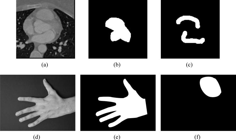
Figure 1 shows an example of training images where the binary images in Figure 1(b,e) are the manual segmentations and the maps in Figure 1 (c,f) show the regions of low confidence and regions which we are not interested in segmenting, respectively. In the cardiac image we see that the neighborhood which contains fuzzy edges have been marked in Figure 1(c) and in the hand image (Figure 1 (f))we eliminate the influence of the segmentation of the thumb to get a better segmentation of the other fingers. These binary images will form our training dataset. Since, this training data is derived from various subjects, the first logical step would be to align these images. This is described in Section 2. In Section 3, we describe the model used for the segmenting curve using shape priors. Section 4 explains how we incorporate the regions of confidence/interest labels into the existing model to improve segmentation. And finally in Section 5 we show the application of this technique to two sets of images.

Figure 1.

(a-c) Cardiac training images. (d-e) Hand images.

2. SHAPE ALIGNMENT

The various images present in the training dataset vary in shape, size and orientation. If we use PCA on this data the variations in size and orientation will mask the shape variations, preventing the PCA from capturing them. Thus, to capture only the shape variations by using shape priors, we first need to align the images in our training dataset with respect to size and orientation. Consider the training set with n binary images {I₁, I₂, ..., I_n} with pose parameters {p₁, p₂, ..., p_n}. For 2D images we define a pose parameter vector p such that p = [a, b, h, θ] with a, b, h and θ correspond to x-, y- translation, scale and rotation, respectively. The transformed image of I, denoted by Ĩ, for a given pose parameter (p) is obtained using a transformation matrix T(p). This transformation matrix T(p) also maps the co-ordinates $(x,y)∊{\mathbb{R}}^2$ to $(\tilde{x},\tilde{y})∊{\mathbb{R}}^2$. The transformation matrix is a product of three matrices: a transition matrix M(a, b), a scaling matrix H(h) and an in-plane rotation matrix R(θ).

$$\tilde{I}=T\left(\mathbf{p}\right)I.$$

where,

$$\left[\begin{array}{c}\hfill \tilde{x}\hfill \\ \hfill \tilde{y}\hfill \\ \hfill 1\hfill \end{array}\right]=\mathrm{T}\left(\mathbf{p}\right)\left[\begin{array}{c}\hfill x\hfill \\ \hfill y\hfill \\ \hfill 1\hfill \end{array}\right]$$

And the transformation matrix, T(p) = MHR, where,

$$M=\left[\begin{array}{ccc}\hfill 1\hfill & \hfill 0\hfill & \hfill a\hfill \\ \hfill 0\hfill & \hfill 1\hfill & \hfill b\hfill \\ \hfill 0\hfill & \hfill 0\hfill & \hfill 1\hfill \end{array}\right],H=\left[\begin{array}{ccc}\hfill h\hfill & \hfill 0\hfill & \hfill 0\hfill \\ \hfill 0\hfill & \hfill h\hfill & \hfill 0\hfill \\ \hfill 0\hfill & \hfill 0\hfill & \hfill 1\hfill \end{array}\right],R\left(\theta \right)=\left[\begin{array}{ccc}\hfill cos\left(\theta \right)\hfill & \hfill -sin\left(\theta \right)\hfill & \hfill 0\hfill \\ \hfill sin\left(\theta \right)\hfill & \hfill cos\left(\theta \right)\hfill & \hfill 0\hfill \\ \hfill 0\hfill & \hfill 0\hfill & \hfill 1\hfill \end{array}\right].$$

As suggested by Tsai et al.⁸ we can jointly align the n images by minimizing the following energy functional:

$$E_{align}=\sum _{i=1}^n\sum _{j=1,j\ne i}^n\left\{\frac{\int {\int }_{\Omega }{({\tilde{I}}^i-{\tilde{I}}^j)}^{2}dA}{\int {\int }_{\Omega }{({\tilde{I}}^i+{\tilde{I}}^j)}^{2}dA}\right\},$$ (1)

where Ω is the image domain and dA is unit area.

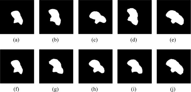
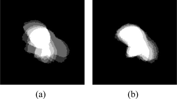
We illustrate the alignment process using five 2-D slices of the segmented epicardium from a training dataset generated using 4-D cardiac scans. These slices were taken from cardiac scans of five different patients, hence the segmentations vary in shape, size and orientation. In Figure 2 we show the cardiac images before and after alignment and in Figure 3 we show the overlay of these images. Here the pose of Figure 2(a) was chosen to be fixed, i.e., p = [0, 0, 1, 0] and the pose parameters for the other images were evolved jointly to align them to this image.

Figure 2.

(a-e) Training images: Five 2-D images from cardiac training data. (f-j) Aligned images: 2-D images from cardiac training data after alignment.

Figure 3.

Comparison of the shape overlay (a) Before alignment. (b) After alignment.

3. SHAPE PRIORS

We will use the level set approach introduced by Osher and Sethian ¹⁰ to represent the shape of the image boundaries. We will represent the shapes using signed distance functions {ψ₁, ψ₂, ...ψ_n}, where the image boundary is embedded as the zero level set and negative distances are assigned to regions inside the boundary and positive distances to regions outside the boundary. Taking the average of the n signed distance functions we get the mean level set for the training images,

$$\stackrel{‒}{\psi }=\frac{1}{n}\sum _{i=1}^n{\psi }_i.$$

We will extract the shape variabilities in each training image by subtracting the mean signed distance function $\stackrel{‒}{\psi }$ from each signed distance function to form n mean offset functions $\{{\widehat{\psi }}_1,{\widehat{\psi }}_2,\dots {\widehat{\psi }}_n\}$.

$${\widehat{\psi }}_i=\stackrel{‒}{\psi }-{\psi }_i.$$

We then form a shape variability matrix $S=\left[{\widehat{\Psi }}_1{\widehat{\Psi }}_2\dots {\widehat{\Psi }}_n\right]$, where the samples of ${\widehat{\psi }}_i$ are stacked lexicographically to form each column ${\widehat{\Psi }}_i$.

As suggested in^8,11 we will take the eigenvalue decomposition of (1/n)S^TS, which will give us the eigenshapes (principal modes), Ψ_i's. For $\{{\widehat{\psi }}_1,{\widehat{\psi }}_2,\dots {\widehat{\psi }}_n\}$ forming the S matrix we will get a maximum of n different eigenshapes {Ψ₁, Ψ₂, ...Ψ_n}. A new level set function can } be expressed as a linear combination of these eigenshapes. For k ≤ n,

$$\tilde{\psi }\left(\alpha \right)=\stackrel{‒}{\psi }+\sum _{i=1}^k{\alpha }_i{\Psi }_i.$$ (2)

where {α₁, α₂, ..., α_k} are the weights associated with the k eigenshapes. We will again use the zero level set of $\tilde{\psi }$ as the representation of our shape. Thus, by varying α, we vary $\tilde{\psi }$ which indirectly changes the shape. The value of k must be chosen large enough to capture the prominent shape variations in the training images. But if the value of k is too large, the model will capture some intricate details that are specific to the images used for training. In all the examples described in this paper we choose the value of k empirically.

The segmentation also needs to accommodate variations in the pose parameters along with the variations in shape. Thus we will include the pose parameters in the representation of the level set function $\tilde{\psi }$ in (2).

$$\tilde{\psi }(\alpha ,\mathbf{p})=\stackrel{‒}{\psi }\left(\mathbf{p}\right)+\sum _{i=1}^k{\alpha }_i{\Psi }_i\left(\mathbf{p}\right).$$ (3)

3.1 Chan-Vese model for segmentation

We will use the region-based curve evolution model described by Chan and Vese ⁴ for segmentation. As explained in⁸ we will use region statistics to evolve the pose parameters (p) and weights of the eigenshapes (α) to vary the segmentation curve. Since, our level set function $\tilde{\psi }$ is a signed distance functions, the segmentation curve $\overrightarrow{C}$ can be represented as the zero-level set of $\tilde{\psi }$,

$$\overrightarrow{C}=\{(x,y)∊R^2:\tilde{\psi }(x,y)=0\}.$$ (4)

The regions inside and outside the curve $\overrightarrow{C}$, denoted respectively by R^u and R^v are given by,

$$\begin{array}{cc}\hfill R^u& =\{(x,y)∊R^2:\tilde{\psi }(x,y)<0\}.\hfill \\ \hfill R^v& =\{(x,y)∊R^2:\tilde{\psi }(x,y)>0\}.\hfill \end{array}$$

For any observed image data denoted by I, the means inside (μ) and outside (ν) the segmentation curve $\overrightarrow{C}$ can be defined as,

$$\begin{array}{cc}\hfill \mu & =\frac{\int {\int }_{\Omega }IH(-\tilde{\psi }(\alpha ,p))dA}{\int {\int }_{\Omega }H(-\tilde{\psi }(\alpha ,p))dA}\hfill \\ \hfill \nu & =\frac{\int {\int }_{\Omega }IH\left(\tilde{\psi }(\alpha ,p)\right)dA}{\int {\int }_{\Omega }H\left(\tilde{\psi }(\alpha ,p)\right)dA}\hfill \end{array}$$

where Ω is the image domain and dA is unit area. And the Heaviside function H is given by,

$$H\left(\tilde{\psi }(\alpha ,p)\right)=\{\begin{array}{cc}1,\hfill & \text{if}\tilde{\psi }(\alpha ,p)\ge 0\hfill \\ 0,\hfill & \text{if}\tilde{\psi }(\alpha ,p)<0\hfill \end{array}\phantom{\}}$$

Using the image statistics defined in this section we can define the Chan-Vese energy functional for segmenting I as,

$$E_{cv}={\int }_{R^u}{(I-\mu )}^{2}dA+{\int }_{R^v}{(I-\nu )}^{2}dA$$ (5)

The 2-D gradient, ∇E_cv can be denoted as,

$$\nabla E_{cv}=F.\overrightarrow{N}$$ (6)

where F for the Chan-Vese model is given by, $F=\{I-\frac{\mu +\nu }{2}\}(\mu -\nu )$

3.2 Parameter Optimization via Gradient Descent

We will use steepest descent on the Chan-Vese energy functional defined in (5) to evolve the pose parameters (p) and the weights (α). We will need the gradient of E_cv with respect to each pose parameter, p_j and shape parameter, α_i. These gradients can be written as,

$${\nabla }_{{\alpha }_i}{E}_{cv}={\int }_C({\nabla }_{{\alpha }_i}C.\nabla E_{cv})ds={\int }_C-\left(\frac{{\nabla }_{{\alpha }_i}\tilde{\psi }}{\Vert \nabla \tilde{\psi }\Vert }\right).Fds,$$ (7)

$${\nabla }_{p_j}{E}_{cv}={\int }_C({\nabla }_{p_j}C.\nabla E_{cv})ds={\int }_C-\left(\frac{{\nabla }_{p_j}\tilde{\psi }}{\Vert \nabla \tilde{\psi }\Vert }\right).Fds.$$ (8)

where s is the arc-length parameter of the curve C. The update equations for the weights and the pose parameters are given by,

$${{\alpha }_i}^{n+1}={{\alpha }_i}^n-{\nabla }_{{\alpha }_i}{E}_{cv}dt,$$ (9)

$${p_j}^{n+1}={p_j}^n-{\nabla }_{p_j}{E}_{cv}dt.$$ (10)

where dt is the step-size and p_jⁿ and α_iⁿ are the values of each pose parameter and weight at the n^th iteration. The new shape and pose parameters are used to update $\tilde{\psi }$ and hence the location of the segmenting curve C after each iteration. Based on the new location of the curve the image statistics μ and ν are recalculated. The derivation of the final forms of (7) and (8) are explained in Appendix - A.

4. REGIONS OF CONFIDENCE/INTEREST

In this section we explain how we incorporate labels of confidence/interest in the model to improve segmentation. As shown in Figure 1, each training image I_i will have a corresponding confidence/interest label image R_i. We will use signed distance functions to represent these images as well. The boundary of the region labeled with low reliability/significance will be our zero level set, the regions inside will be assigned negative values and the regions outside will be assigned positive values. Thus we will form a new set of signed distance functions, {L₁, L₂, ..., L_n}, where negative values indicate regions with low reliability/significance. With these signed distance functions we will form a new shape variability matrix S, which will include these labels,

$$\mathrm{S}=\left(\left[\begin{array}{c}\hfill {\widehat{\Psi }}_1\hfill \\ \hfill {\widehat{L}}_1\hfill \end{array}\right]\left[\begin{array}{c}\hfill {\widehat{\Psi }}_2\hfill \\ \hfill {\widehat{L}}_2\hfill \end{array}\right]\cdots \left[\begin{array}{c}\hfill {\widehat{\Psi }}_n\hfill \\ \hfill {\widehat{L}}_n\hfill \end{array}\right]\right).$$

Here the samples of each signed distance function L_i are stacked lexicographically to form the corresponding 1-D array ${\widehat{L}}_i$. Taking the eigenvalue decomposition of this S matrix will give us n eigenshapes {Ψ₁, Ψ₂, ...Ψ_n} and their corresponding eigenlabels {l₁, l₂, ..., l_n}. These eigenlabels can be used to improve the final segmentation by influencing the update on pose parameters (p) and the weights (α) and thus influencing the curve evolution. For this we will take a linear combination of the eigenlabels to form a new level set function for the labels l, similar to the level set formed in (2).

$$l(\alpha ,\mathbf{p})=\stackrel{‒}{l}\left(\mathbf{p}\right)+\sum _{i=1}^k{\alpha }_i{l}_i\left(\mathbf{p}\right),$$ (11)

where k ≤ n and {α₁, α₂, ..., α_k} are the weights associated with the k eigenlabels. The variable l̄ is the mean of the n signed distance functions which is defined as,

$$\stackrel{‒}{l}=\frac{1}{n}\sum _{i=1}^n{L}_i.$$

Incorporating this new label function l in calculating the gradients of the energy functional E_cv with respect to each pose parameter p_j and shape parameter α_i we get,

$${\nabla }_{{\alpha }_i}{E}_{cv}={\int }_{C}l({\nabla }_{{\alpha }_i}C.\nabla E_{cv})ds={\int }_C-l\left(\frac{{\nabla }_{{\alpha }_i}\tilde{\psi }}{\Vert \nabla \tilde{\psi }\Vert }\right).Fds,$$ (12)

$${\nabla }_{p_j}{E}_{cv}={\int }_{C}l({\nabla }_{p_j}Cl\nabla E_{cv})ds={\int }_C-l\left(\frac{{\nabla }_{p_j}\tilde{\psi }}{\Vert \nabla \tilde{\psi }\Vert }\right).Fds.$$ (13)

The amount of influence of each pixel on the evolution of the curve is now governed by the value of l. Since negative values of l at a given pixel indicates low confidence or significance, we will not include these pixels in our calculation. The values of each shape parameter α_i and pose parameter p_j are updated iteratively using the equations (9) and (10) respectively. These updated weights are used to calculate the new level set function $\tilde{\psi }$ in (3) and the new label function l in (11) after each iteration.

5. RESULTS

We apply the model described in the previous sections to two sets of images: 1) Cardiac MRI data and 2) Hand images. We also compare the results generated in using the model with and without the aid of regions of confidence/interest labels.

5.1 Segmentation of Cardiac CT data

We compare the segmentation of the myocardium on 2D cardiac slices using shape priors as explained in ^8,11 with our technique of using shape priors along with the regions of confidence labels. Fifteen slices from a 4-D interactive segmentation of cardiac data from a single patient form our training dataset. Along with the manual segmentation on these slices we also have corresponding images that mark the regions of low confidence. Figure 4 shows the raw data, manual segmentation and regions of low confidence of one such slice from the training dataset.

Figure 4.

(a) Raw Image. (b) Manual segmentation with Regions of low confidence. (c) Regions of low confidence for epicardium. (d) Regions of low confidence for endocardium.

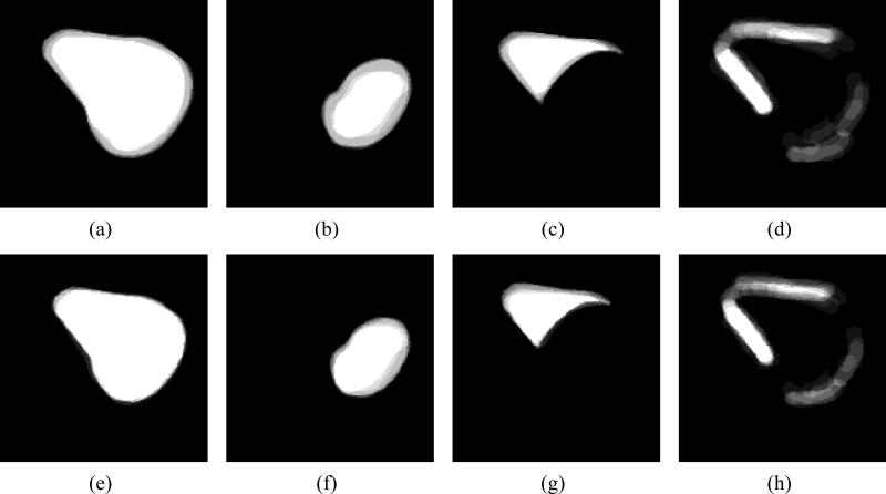
Our target segmentation curve should form the boundary of the two ventricles and the epicardium. Representing this curve using a single level set would make the model susceptible to harmful topological changes such as merging of the inner and outer walls of the myocardium (especially in the regions where the myocardium is very thin). Thus, we represent each ventricle and the epicardium as a separate curve with three different signed distance functions associated with each of them. Our training dataset thus consists of images that represent the two ventricles, epicardium and corresponding maps indicating regions of low confidence. Figure 5 shows an overlay of the aligned training images. Here we use a single combined pose parameter p to align the ventricles and the epicardium. This way we can prevent the curves from crossing each other. The same pose parameters are also used to align the regions of low confidence.

Figure 5.

Overlay of training images for epicardium, left ventricle, right ventricle and Region of low confidence (a-d) before alignment (e-h) after alignment.

We derive eigenshapes for each region (left ventricle, right ventricle and epicardium) and their corresponding eigenlabels by performing a PCA as explained in Section 3. Since the regions were aligned using a single set of pose parameters, we will also take a combined PCA of these regions. We chose a value of k=5 to generate these results.

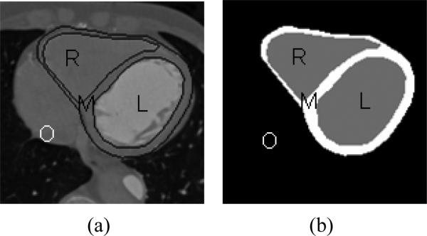
Figure 6(a-b) shows the manual segmentation on a 2-D slice consisting of four regions marked as L, R, M and O which represent the left ventricle, right ventricle, myocardium and region outside the epicardium respectively. The three curves used for segmentation will divide the observed image data (I) into these four regions. Since the image is now divided into multiple regions, we introduce a new coupled energy functional, E_coupled.

$$E_{coupled}={\int }_L{(I-u_L)}^{2}dA+{\int }_R{(I-u_R)}^{2}dA={\int }_M{(I-u_M)}^{2}dA+{\int }_O{(I-u_O)}^{2}dA.$$

Figure 6.

Images showing manual segmentation of cardiac 2-D slices which are differentiating into 4 regions: Left ventricle, Right ventricle, Myocardium and Outside region.

We evolve the parameters p and α by minimizing E_coupled using image statistics based on these four regions. u_L, u_R, u_M, u_O represent the means inside the regions L, R, M, O respectively and dA is the unit area.

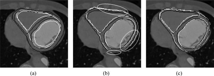
Figure 7 shows the segmentation results, and compares each result with the manual segmentation. The white contour is the curve we obtained in our segmentation and the black contour indicates the ground truth (manual segmentation) for that particular slice. We can see that using regions of confidence labels significantly improves the segmentation within the highlighted sections. Since, this approach uses global parameters to evolve the curve, our approach shows improvement in segmentation even in the regions containing strong edges.

Figure 7.

(a) Initialization of segmentation using the zero level set of $\stackrel{‒}{\psi }$. (b) Segmentation results using shape priors. (c) Segmentation enhanced with use of Regions of confidence.

5.2 Segmentation of hand images

In this example we take hand images, with varying positions of the fingers. Our training dataset for this example consists of 5 images. Once we align the training images, the palms of all the images in our training datasets will be aligned. Thus the PCA will be able to capture the variation in the shape, size and position of the fingers. The initial overlay of these hand images are shown in Figure 8(a) and Figure 8(b) shows an overlay of the aligned hand images. We also generate two sets of regions of interest here, one masking the thumb and the other masking the last three fingers in each hand. Because the thumb finger shows a large variation in position, masking the thumb out while segmenting the other fingers will improve the overall segmentation of the other fingers. And in the second set, we mask out the last three fingers to segment the thumb. If we mask all the four fingers, there is a possibilty that the final segmentation rotates the entire palm to fit the thumb. To avoid this we leave the index finger out of the mask to give the segmentation some information about the location of the palm. Figure 8(c,d) show the mean images of the regions of interest masking the thumb region and the last three fingers.

Figure 8.

(a) Overlay of hand images before alignment. (b) Overlay of aligned hand images. (c) Aligned regions of interest label masking the thumb. (d) Aligned regions of interest label masking the last three fingers.

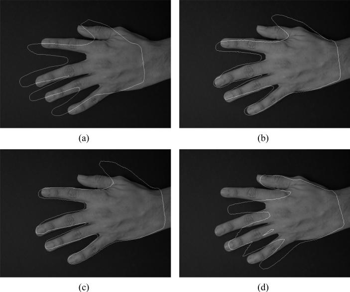
We use shape priors to segment the hand image as explained in Section 3. The initializing curve obtained from the zero level set of $\stackrel{‒}{\psi }$ of the training data is shown in Figure 9(a). The result generated by shape priors as explained in ⁸ is shown in Figure 9(b). Figure 9(c,d) show the results generated by using the two sets of region of interest masks generated. We chose a value of k=3, in all these examples. We see that in Figure 9(b) the curve tries to capture the variations in thumb as well as the fingers, and fails to segment them very well. But by masking the thumb we get a very good segmentation of the other fingers, although the thumb segmentation is worse than in the previous case(Figure 9(c)). In Figure 9(d), by masking the last three fingers we get a good segmentation of the thumb, but in the process we deteriorate the quality of segmentation along the other fingers. Thus by using these separate masks we can selectively improve segmentation in certain regions of the image.

Figure 9.

(a) Initialization of segmentation using the zero level set of $\stackrel{‒}{\psi }$. (b) Segmentation results using shape priors. (c) Segmentation of the fingers with the regions of interest masking the thumb. (d) Segmentation of the thumb with the regions of interest masking the last three fingers.

6. CONCLUSION AND FUTURE WORK

In this paper we have presented a novel technique that uses labels of confidence/interest to enhance the existing region based shape prior segmentation model. We have described how we can selectively exclude the influence of certain neighborhoods in segmenting the curve and thus improve the quality of segmentation. We show how this technique can improve segmentation in medical images, not only along the regions with fuzzy edges but also in the regions with prominent edges. We also show how we can get higher quality segmentation in certain parts of the image by ignoring regions in the image which we are not interested in. The results presented in the paper show how we can use this model to separately improve segmentation in various portions within a single image using fewer training images. We are currently working on ways to combine these separate regions with high quality segmentations to obtain a single segmenting curve on the entire object.

APPENDIX A

In this section we explain how we can simplify the equations (7) and (8) to express the gradients ∇_αiE_cv and ∇_pjE_cv in terms of the level set function and image statistics. The segmentation curve is embedded as the zero-level set of the function $\tilde{\psi }$. Since, $\tilde{\psi }$ is a function of the curve C, weights α and pose parameters p; the curve C (zero level set) will also be a function of α and p along with the arc-lenght parameter s. Hence the zero level set can be represented as,

$$\tilde{\psi }(C(\alpha ,\mathbf{p},s),\alpha ,\mathbf{p})=0.$$

Taking derivative of with respect to α_i we get,

$${\nabla }_{{\alpha }_i}\tilde{\psi }+\Vert \nabla \tilde{\psi }\Vert \cdot \overrightarrow{N}\cdot {\nabla }_{{\alpha }_i}C=0$$

We thus have,

$${\nabla }_{{\alpha }_i}C.\overrightarrow{N}=-\frac{{\nabla }_{{\alpha }_i}\tilde{\psi }}{\Vert \nabla \tilde{\psi }\Vert }$$ (14)

Now the gradient of the energy functional E_cv with respect to α_i is defined in (7) as,

$${\nabla }_{{\alpha }_i}{E}_{cv}={\int }_C\left({\nabla }_{{\alpha }_i}C.F.\overrightarrow{N}\right)ds$$ (15)

Substituting, the value of ∇_αiC. $\overrightarrow{N}$ from (14) we have,

$${\nabla }_{{\alpha }_i}{E}_{cv}={\int }_C-\left(\frac{{\nabla }_{{\alpha }_i}\tilde{\psi }}{\Vert \nabla \tilde{\psi }\Vert }\right).Fds.$$ (16)

Similarly, for the gradient of E_cv with respect to p_j will be,

$${\nabla }_{p_j}{E}_{cv}={\int }_C-\left(\frac{{\nabla }_{p_j}\tilde{\psi }}{\Vert \nabla \tilde{\psi }\Vert }\right).Fds.$$ (17)

Thus in calculating the update for each parameter in equations (9) and (10) we only need the gradients of the signed distance function with respect to that parameter and the value of F along the line integral of C. The image statistics μ and ν need to be calculated only once after each iteration. This makes the model simple to implement and computationally efficient.

REFERENCES

- 1.Chen Y, Thiruvenkadam S, Huang F, Wilson D, Md EAG, Tagare HD. On the incorporation of shape priors into geometric active contours; Variational and Level Set Methods in Computer Vision, IEEE Workshop on; 2001. pp. 145–152. [Google Scholar]
- 2.Leventon M, Grimson E, Faugeras O. Statistical shape influence in geodesic active contours; [Proc. of Computer Vision and Pattern Recognition CVPR 2000]; 2000. [Google Scholar]
- 3.Mumford D, Shah J. Optimal approximations by piecewise smooth functions and associated variational problems. Communications on Pure and Applied Mathematics. 1989;42(5):577–685. [Google Scholar]
- 4.Chan T, Vese L. An active contour model without edges; [Int. Conf. Scale-Space Theories in Computer Vision]; 1999. pp. 141–151. [Google Scholar]
- 5.Chan TE, Vese LA. A level set algorithm for minimizing the mumford-shah functional in image processing; [IEEE WORKSHOPon Variational and Level Set Methods in Computer Vision]; p. 161168. [Google Scholar]
- 6.Cremers D, Tischhauser F, Weickert J, Schnorr C. Diffusion snakes: Introducing statistical shape knowledge into the mumford-shah functional. 2002 December;50:295–313. [Google Scholar]
- 7.Tsai A, Yezzi A, Willsky A. A curve evolution approach to smoothing and segmentation using the mumford-shah functional. 2000:119–124. I. [Google Scholar]
- 8.Tsai A, Yezzi A, Wells W, Tempany C, Tucker D, Fan A, Grimson WE, Willsky A. A shape-based approach to the segmentation of medical imagery using level sets. [Medical Imaging, IEEE Transactions on], IEEE transactions on medical imaging. 2003 February;22:137–154. doi: 10.1109/TMI.2002.808355. [DOI] [PubMed] [Google Scholar]
- 9.Cremers D, Sochen N, Schnrr C. Multiphase dynamic labeling for variational recognition-driven image segmentation. [In ECCV 2004, LNCS 3024] 2004;74–86 Springer. [Google Scholar]
- 10.Osher S, Sethian JA. Fronts propagating with curvature dependent speed: Algorithms based on hamilton-jacobi formulations. JOURNAL OF COMPUTATIONAL PHYSICS. 1988;79(1):12–49. [Google Scholar]
- 11.Abufadel A, Yezzi T, Schafer R. 4d segmentation of cardiac data using active surfaces with spatiotemporal shape priors. Comp Imaging. 2007;6498(1) SPIE. [Google Scholar]