Solutions for a local equation of anisotropic plant cell growth: an analytical study of expansin activity

Abstract

This paper presents a generalization of the Lockhart equation for plant cell/organ expansion in the anisotropic case. The intent is to take into account the temporal and spatial variation in the cell wall mechanical properties by considering the wall ‘extensibility’ (Φ), a time- and space-dependent parameter. A dynamic linear differential equation of a second-order tensor is introduced by describing the anisotropic growth process with some key biochemical aspects included. The distortion and expansion of plant cell walls initiated by expansins, a class of proteins known to enhance cell wall ‘extensibility’, is also described. In this approach, expansin proteins are treated as active agents participating in isotropic/anisotropic growth. Two-parameter models and an equation for describing α- and β-expansin proteins are proposed by delineating the extension of isolated wall samples, allowing turgor-driven polymer creep, where expansins weaken the non-covalent binding between wall polysaccharides. We observe that the calculated halftime (t_1/2 = εΦ₀ log 2) of stress relaxation due to expansin action can be described in mechanical terms.

1. Introduction

The Lockhart [1] equation has gained a prominent place among the key milestones in the field of plant growth mechanics. This model, however, in its raw form, has many shortcomings that limit its usefulness. These include the formulation of uniaxial cell growth, when in fact cell growth involves strain rates along three directions. Moreover, the mechanical anisotropy of the cell wall was completely ignored. This latter aspect has been considered by many authors, and recently a local (coordinate-dependent) tensor growth equation was developed to address the problem of phototropism [2] and gravitropism [3]. Yet, there is still a need for an all-encompassing local equation of volumetric cell/organ growth complemented by a space- and time-dependent cell wall extensibility coefficient, retaining positive aspects of the original Lockhart equation.

The extensibility coefficient (Φ₀) was originally defined as a constant; however, it should be non-constant to address the changes taking place in the walls of the growing plant cell. It should have directional dependence as well. Also, numerous experiments provided evidence that the extensibility coefficient is susceptible to many environmental stimuli. These include phytohormones or growth inhibitors and temperature, and especially a time-dependent change in the value of the extensibility coefficient. From a purely mathematical point of view, not to mention a huge body of observational data, the extensibility coefficient magnitude should gradually decrease with time, ceasing altogether when the cell matures. In fact, the conventional treatment of the Lockhart equation (with Φ₀ = const.) delivers exclusively an exponential solution for the expanding cell volume V, which is clearly flawed.

In this paper, a consistent solution of anisotropic plant cell/organ growth is presented in the form of a dynamic tensor equation. The latter is supplemented by an important application to the role of expansin proteins in the problem of cell wall extension.

2. Results

2.1. Theory

The Lockhart equation in its original form is given by

2.1

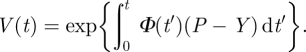
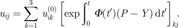
where V denotes the volume of a growing cell. In equation (2.1), P and Y describe the turgor pressure and turgor threshold, respectively; the constant Φ₀ stands for the ‘extensibility’ coefficient. The formal solution of equation (2.1) gives V = V₀e^{Φ₀(P−Y)t}, where V₀ = V(t = t₀) is the initial volume. In a more general case, Φ₀ is time-dependent (e.g. [4]), Φ₀ → Φ(t), and then the integration of equation (2.1) gives

2.2

An even more general treatment of the extensibility coefficient Φ₀ demands space- and time-dependence: Φ₀ → Φ(t, x₁, x₂, x₃). As noted elsewhere [2], the condition is that the local equations should reproduce the global ones by assuming homogeneity and isotropy, but we may, nonetheless, formally introduce the dynamic tensor equation in the form

2.3

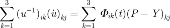
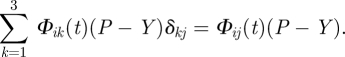
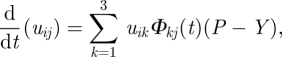
(the lower indices i, j and k take values 1, 2 and 3 for the cartesian coordinates, e.g. we use x₁, x₂ and x₃ notation instead of the usual x, y, z, respectively; the summation is performed over repeating indices, here: k = 1,2,3) representing the anisotropic cell growth owing to the internal stress field¹ (figure 1). In equation (2.3), where u_ij = ξ_i,j + ξ_j,i ≡ {∂ξ_i/∂x_j + ∂ξ_j/∂x_i}, the left side stands for the dynamic deformation of the cell volume, while (P − Y)_ij denotes the stress field caused by the turgor pressure; ξ =(ξ₁, ξ₂, ξ₃) is the displacement vector within the time interval Δt = t′ − t; dot represents, as usual, the time derivative. Strictly speaking, ξ_i,j = ∂ξ_i/∂x_j represents the rate of change of the ith component of vector ξ in x_j direction. Coefficient Φ_ik(t) corresponds to the dynamic intrinsic extensibility due to biochemical reactions taking place in the cell wall and is represented by a second rank tensor. Assuming the cell sap as an incompressible fluid, and making use of Pascal's principle, which states that pressure applied to a confined fluid at any point is transmitted undiminished through the fluid, then

2.4

where δ_ij stands for the Kronecker delta function. Thus, we may rewrite the right side of equation (2.3) in the following manner:

2.5

Figure 1.

Schematic diagram of a plant cell undergoing stress due to internal pressure. Stress in a loaded deformable cell wall is assumed to be a continuum. Stress at any point in an object, assumed to be a continuum, is completely defined by the nine components of a second-order tensor known as the Cauchy stress tensor, σ (here P − Y). (Online version in colour.)

Then, after inserting this result into equation (2.3), it takes the form

2.6

and corresponds to equation 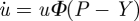in matrix form. Equation (2.6) can be solved to receive

2.7

The biochemical aspect of cell wall extension can be recalled [4] when considering the right-hand side of equation (2.7). In the simplest approximation, the change in the number of expansin proteins in the investigated system will be proportional to concentration x and to the kinetic coefficient k₀ responsible for the interaction of endogenous expansins with the cell wall. Initial efforts started with a time-differential equation for the kinetic chemical reaction with 0 ≤ x ≤ 1 − expansin concentration in the growing hypocotyl/coleoptile fragment, and k₀ is the kinetic coefficient (responsible for chemical reaction rate) bound with expansin interaction with the growing segment, leading to stress relaxation in the expanding wall. The differential equation was integrated to yield x(t) = x₀ exp(−k₀t), where x₀ = x(t = 0) stands for the initial expansin concentration of the investigated system. This latter equation describes the exponential degradation of an initial pulse of the cell wall loosening by expansins. This approach also suggests a mechanism for finite cell extension: the cell becomes rigid as the initial pulse of stress-relaxing expansin protein expires. The above argument implies that the latter solution may be treated as a modifying factor for Φ₀. Thus, we substituted Φ(t) → Φ₀x(t), to obtain

2.8

where Φ₀ = const. is the original (Lockhart) coefficient.

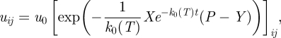
Assuming the rules imposed by growth geometry (principal growth directions) and spatially inhomogeneous concentration x₀ leading to the relation [x₀ exp(−k₀t)]_ij=x₀^ij exp(−k₀t), substituting Φ(t) → Φ_ij(t) = x₀^ij exp(−k₀t) and performing insertion into equation (2.7) we arrive, after integration over time variable, at (henceforth Φ₀ = 1) the local solution

2.9

where X = (x₀^ij) (i,j = 1,2,3) is a matrix,² u₀ = exp[c] = const. and can be determined by initial conditions. The bracket […]_ij represents the following properties: the diagonal elements […]_ii are normal stresses (i.e. perpendicular to the corresponding surfaces), while the off-diagonal elements […]_ij, i ≠ j are the tangential stresses. The solutions of equation (2.9) are continuous functions of X matrix (in fact X represents a stress field). Obviously, by assuming isotropic conditions, taking the trace operation on equation (2.9) and by using ξ_i,i = div(ξ) = dV/V, we return to the global equation.

The above equation can be applied easily to the principal growth directions of plant cells, organs, roots or shoots. The approach also takes into account a non-homogeneous distribution of expansin proteins that has been reported (e.g. [6]). This equation, in contrast to kinematic considerations presented by other authors, is a fully dynamic tensor equation, including some of the basic forces (turgor pressure, turgor threshold) involved. Furthermore, the environmental temperature, decisive for growth processes, can be taken into account by a well-justified assumption that k₀ = k₀(T), where T stands for the absolute temperature. The effect of temperature on rates of reaction for a given plant species can be easily established empirically (cf. [4]; see fig. 8 and footnote 2 therein). There, the kinetic coefficient k₀ for maize (Zea mays L.) changes in the interval of 20–30°C about two times. This is in good agreement with the ‘Q10 law’ stating that the rate at which the chemical reaction proceeds will approximately double for each 10°C increase in temperature (for plants, for obvious reasons, there is some variability: for maize it was found that this ratio is about 1.8 [4]).

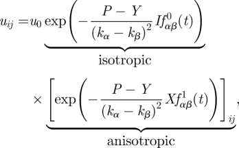
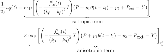
Since we are seeking here the most general semi-phenomenological equation of growth, we may advance one step further by accepting, as an example, one of a two-parameter models (for details, see the derivation of equations (2.22) and (2.25)), describing α- and β-expansin protein participation in the cell wall loosening and relaxation process. Similar procedures, as in the case of equation (2.9), can be performed to give a deformation field due to internal stress field in the form

2.10

where f_αβ⁰(t) =−k_β + e^{(k_β−k_α)t}k_β + k_αk_βt − k_β²t, f_αβ¹(t) = −k_α+e^{(k_β−k_α)t}k_α + k_β − e^{(k_β−k_α)t}k_β and I stands for the identity (diagonal) matrix. The resulting local solution has two terms, namely isotropic and anisotropic (see also figure 2). The first term can be recognized as originating from the Lockhart-type (isotropic) term, while the second term can be considered as an anisotropic correction to growth. Direct calculation transforms equation (2.10) to equation (2.9) by assuming k_α = k₀ and k_β = 0. Obviously, as in equation (2.9), in general we have k_α = k_β(T) and k_β=k_β(T). The method of how to assign experimentally based values to the kinetic coefficients (k_α and k_β) is described in detail in §3.

Figure 2.

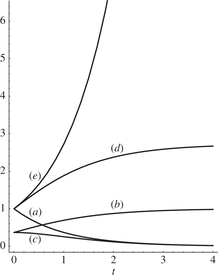
Plot of the functions entering equations (2.1)–(2.10) and equation (3.2): (a) exp(−t), (b) exp(−exp(−t)), (c) its derivative exp(−t − exp(−t)), (d) exp(1 − exp(−t)) and (e) the divergent solution of equation (2.1) exp(t), as a function of time.

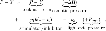
Hitherto, we have considered and rearranged the cell wall ‘extensibility’ term in equation (2.1). Now, we reconsider the pressure term (P − Y). In the following, we will assume constant water uptake, since the case where a plant is deprived of water sources has already been delineated previously [4]. In our recent paper [7], we have considered the dynamic balance between the water uptake and cell wall yielding mainly by considering the pressure term and taking into account an auxiliary Lorentz-like distribution. There, we also considered the environmental temperature T as one of the main abiotic factors influencing growth. We put forward the hypothesis that some other external factors, like stimulators/inhibitors or light-influencing growth, should be present in the pressure term (figure 3). Therefore, we accepted the right side of equation (2.1) and performed the following substitution

2.11

where p₁ (stimulator: p₁ > 0, inhibitor: p₁ < 0) and p₂ represent intracellular pressures relevant to the growth-influencing stimulators/inhibitors, and to the phytochrome-mediated growth retardation upon irradiation with incident light, respectively. The osmotic pressure ΔΠ term may also be used when needed. The function θ stands for the Heaviside theta distribution, which is coupled to the stimulator (+) or inhibitor (−) switch at a time t₁. The external pressure term can be adopted in various extensometric experiments by substituting P_ext = Mg/S, where the nominator represents the load (tension) and S represents the relevant cross-section surface. (The model of linear/nonlinear growth response including light radiation, and the energy irradiation has been developed in extenso elsewhere [7].) Now, we may merge both approaches, represented by equations (2.10) and (2.11), into one all-encompassing thermodynamic tensor equation

2.12

representing plant cell/organ growth at a given temperature T, in either acidic or neutral pH, influenced by internal (biochemical: α- and β-expansin proteins) and external (chemical: growth stimulator/inhibitor or physical: pressure or light) factors. This equation takes into account both the existing anisotropies and inhomogeneities in expansin distribution in the volumetrically growing cell/tissue region, but can also be reduced to a much simpler isotropic form. Temperature, decisive for growth processes, enters this equation in several places: (i) the kinetic coefficients k_α = k_α(T) and k_β = k_β(T), connected with cell wall properties [4],³ (ii) the effective pressure term P − Y through the state equation P(T,V) ∝ T/V (or just P ∝ T), valid from low temperatures to the optimum growth temperature T* (e.g. [7,14]), and (iii) the ‘light’ term through the integral over Planck's distribution ([7], eqn (17)) in the optical range (OR), where the efficiency of this process can be taken into account by inserting the coefficient η ∈ [0,1] in the right-hand side of this equation. Obviously, we may always omit some additive terms in equation (2.12) irrelevant for a given experiment.

Figure 3.

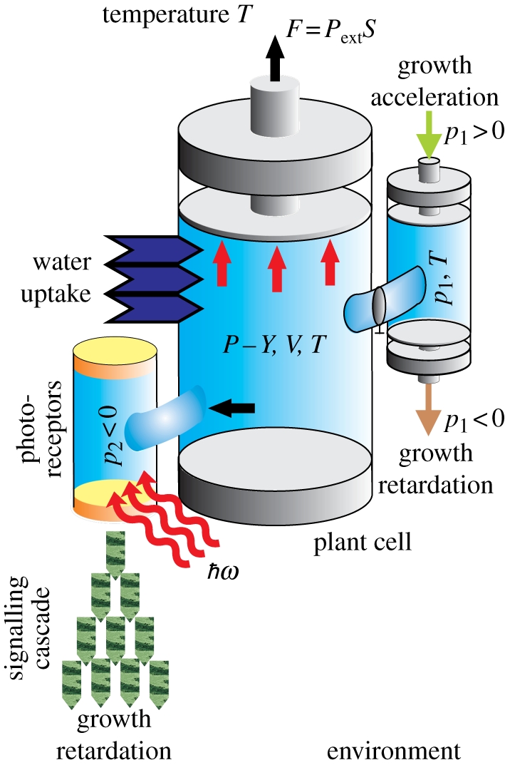
Illustration for equations (2.11) and (2.12): Movement of the piston in the cylinder reflects the isotropic effective pressure, due to Pascal's principle, inside the vacuole (the osmotic pressure difference ΔΠ is not indicated). The container with pressure p₁ and a valve which can be opened at a time t = t₁ is bound with the action of a growth stimulator p₁ > 0 or inhibitor p₁ < 0. An additional container with pressure p₂ represents the (negative) influence of light on the elongation growth (the incident light quanta of energy ℏω are absorbed by photoreceptors and induce a signalling pathway that ultimately leads to growth retardation). The (possible) external mechanical pressure acting on the plant cell is represented by the applied force, F. The whole system (the plant cell/organ) is immersed into a thermostat (environment) at the absolute temperature, T. (Online version in colour.)

2.2. Application to expansins: an isotropic case

A novel class of cell wall loosening proteins called expansins was discovered 20 years ago, and evidence continues to accumulate for their important role in plant cell growth [15–17]. Expansins are plant proteins that mediate changes in cell wall plasticity during cell extension or differentiation (e.g. [16,17]). Expansins appear to have the capacity to induce extension in isolated cell walls and are thought to mediate pH-dependent cell enlargement. Expansin proteins have been identified as wall-loosening factors and as facilitators of cell expansion in vivo and are generally accepted to be the key regulators of wall extension during plant growth.

Expansins are a superfamily of plant proteins involved in cell wall extension and stress relaxation, abscission, fruit softening, the response to biotic and abiotic stresses, and development of leaf, floral organ, root hairs and grain size [8,9,17–28]. Expansins are subdivided into four families: α-expansin, β-expansin, expansin-like A and expansin-like B [29]. The proteins typically have a length of 250–275 amino acids and contain a signal peptide and two domains. Domain 1 has homology to glycoside hydrolase family 45 proteins, which are fungal β-1,4-d-endoglucanases [29]. Domain 2 has homology to G2A proteins, and is hypothesized to bind cell wall polysaccharides [29]. Cell wall modification has been experimentally measured for α-expansin and β-expansin proteins, whereas expansin-like A and expansin-like B proteins are identified as family members only because of the gene sequence. α-Expansin and β-expansin proteins have been implicated in cell growth stimulation at low extracellular pH (acid-growth), and are thought to loosen cell walls via a non-enzymatic mechanism that induces slippage of cellulose microfibrils [16,24,29–34]. This action is presumed to occur by disruption of hydrogen bonds between the cellulose polysaccharides in cell walls strained mechanically by turgor pressure [31]. The cessation of cell growth during development and differentiation appears to be due to a loss of cell wall sensitivity to expansin activity [35,36].

The experimental procedure to detect expansin activity follows several steps [15,24]. The heat-inactivated plant cell walls are excised from the growing region of young seedlings, abraded and clamped at constant axial load in an extensometer coupled to the linear variable differential transformer position transducer, which then measured changes in the length of the wall specimen (see also fig. 1 in [16]). Expansin proteins were collected from growing cells and extracted for wall proteins. These, in turn, were added to the solution surrounding the wall sample (figure 4).

Figure 4.

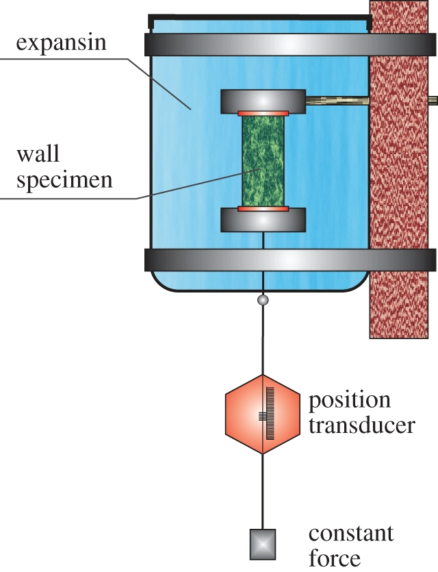
Schematic diagram of a plant cell wall extension assay to detect expansin activity, based on Cosgrove's original experimental procedure and published works [15,24]. Expansin proteins collected from growing cells and extracted for wall proteins are added to the solution surrounding the wall sample. The position transducer measures changes in the length of the wall specimen undergoing stress owing to external pressure (constant load Mg). The control assay (not indicated) represents the identical apparatus with pure water substituting the expansin solution. (Online version in colour.)

To model the above-described experiment in mathematical terms, several ingredients are required. A new equation that is able to describe the basic cell wall mechanical properties for elastic and plastic deformation was introduced previously [4]. This generalization of the canonical Lockhart equation retains the proportionality of the turgor pressure P exceeding the turgor threshold Y and the relative volume change defined as 1/V dV/dt. However, in the generalized Lockhart equation, the extensibility coefficient Φ₀ is treated as time-dependent (cf. equation (2.2)) instead of as a constant. We develop a biochemical approach that is a simple time-differential equation of the kinetic reaction for expansin activity, and incorporate it into the mechanical approach. We briefly review the previously published one-parameter model [4], and introduce 2 two-parameter models with special emphasis on the dynamical description of α- and β-expansin protein activity. By introducing relevant concentrations and kinetic coefficients for α- and β-expansins and superimposing a completeness constraint, we describe the effect of the parameters on the expansin concentration and decay (and the opposite) in our model. In all cases mentioned above, an exact solution of growth equation is found. Also, in these situations where excess fluid (as occurs in experiment) is squeezed out of the cell wall volume, we put P − Y, representing the relative turgor pressure, as equal to zero, in order to map ex vivo creep.

The final equations of the volumetric expansion, as produced by both biomechanical and biochemical approaches, may be calculated to include growth rate (GR) and creep rate (CR). An analytical solution to differentiate both GR and CR, which may address some long-lasting controversy, is then proposed. We take the simplest one-parameter biochemical model equation to show which GR and CR process dominates in the course of time. We conclude with the statement about the possible link between biochemical and biomechanical aspects of growth (or wall creep) by showing some useful analytical relations connecting the two. We also stress that the final solutions resulting from both the methods not only describe the experimental assay but also, in an almost unchanged manner, may serve to characterize the action of endogenous expansins on cell wall loosening and consequent expansion. In all considerations, we are restricted to homogeneous expansin distribution in the specimen under study.

2.2.1. Biomechanical model

To find an analytical description of the experimental studies on plant cell wall creep and growth in the framework of the biomechanical model, consider the model Ansatz as a time-differential equation for the cell wall extensibility coefficient, Φ [4]

2.13

describing the elastic and plastic features of the wall (strictly speaking, in the non-isotropic case, Φ should be a second-rank tensor). Time-dependent wall extensibility seems to be a reasonable assumption—during growth, plant cells secrete a protein called expansin, which unlocks the network of polysaccharides, permitting turgor-driven cell enlargement. We assume that the cell wall behaves as governed by a damped motion equation (2.13), with wall elasticity acting as a restoring force, an inertial wall mass and a viscotic friction due to plastic deformation of the wall. In equation (2.13), λ = b/m and , where b is the viscous damping (reflecting changes in wall plasticity of the expanding cell), k is the restoring (elastic) constant and m the specimen mass (we may always put m = 1 to set the unit system and get rid of the third (m) parameter). The prime denotes, as is usual, the time derivative.

The general solution of equation (2.13) for λ²> ω₀² takes the form of aperiodic damping [4]

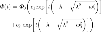2.14

where c₁ and c₂ are constants determined by the initial conditions and Φ₀ = const. is the original (Lockhart) coefficient. Assuming the generalized form of the Lockhart [1] equation for the expanding volume V, with extensibility coefficient Φ as being time-dependent, Φ = Φ(t)

2.15

introducing an external constant force Mg (corresponding to extensometer uniaxial load) in the form of applied pressure, and incorporating equation (2.14) into equation (2.15), we get

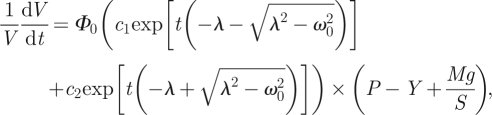2.16

where M is the attached mass and S the horizontal cross-section surface of the investigated coleoptile/hypocotyl fragment; acceleration due to gravity, g = 9.81 m s⁻². This differential equation can be integrated to produce the solution in the form

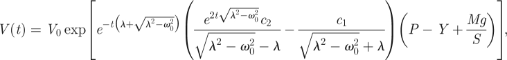2.17

where V₀ denotes the initial volume (Φ₀ may be just considered as a convenient scaling factor, and may be omitted by setting to unity: Φ₀ = 1). The resulting formula, equation (2.17), represents the volumetric expansion of a cell or non-meristematic tissue (no cell divisions) in the course of time with an additional (external) pressure present. We may obviously put P − Y = 0 in equation (2.17) when considering cell wall mechanical properties itself. For a possible quantitative description of expansin activity in the isolated cell wall extension assay as in figure 4 (P − Y = 0), equation (2.17) may serve as a good candidate. This can be accomplished under the justified assumption of this expansin activity being proportional to the investigated specimen wall surface area (because of interactions). To be precise, we propose equation (2.17) (with P − Y = 0) as able to describe the change in the cell/organ volume due to expansins in case of application of an external force Mg in the framework of mechanical approach.

2.2.2. Biochemical model

Two wall proteins, expansin [16] and yieldin [37], are known to be involved in acid-facilitated wall extension. The biochemical mechanism of cell wall-loosening underlying elongation growth of plant organs represents an unsolved problem and is still a matter of current debate. Hence, we put forward some ideas in the following biochemical models.

2.2.2.1. The one-parameter model

In the simplest approximation [4], the change of expansin content in the investigated system will be proportional to its initial (t = 0) concentration x₀ in the solution and to the kinetic coefficient k₀ (proportional to the reaction rate), responsible for the interaction of expansins with the investigated sample.

There [4], we arrived at the formula (for brevity, we put Φ₀ =1 onwards, but in all applications it must be resumed because of its dimensionality and order of magnitude: (1/MPa s) = 10⁻⁶ (1/Pa s))

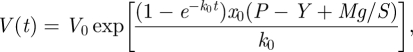2.18

where the initial condition V(t = 0) = V₀ has been used. In the above equation, the external force term Mg has been added to reflect the experimental conditions (figure 4). The above equation can be considered, similar to equation (2.17), as for volumetric extension of a cell/tissue under the tension of an uniaxial force (as before, we need to put P − Y = 0, corresponding to cell fluid being squeezed out, to consider the wall properties itself).

However, as we also want to address the problem of GR versus CR analytically, we need to perform one more calculation. Namely, we need to take the time derivative of equation (2.18) to receive the GR. Thus, another calculation delivers

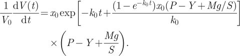2.19

Equation (2.19) represents the GR (P − Y > 0) or CR (P − Y = 0).

However, in order to describe more complicated experimental situations, the extension of the one-parameter model may be unavoidable. Additional effects (e.g. creation/annihilation of expansins or the possible coexistence of expansin proteins of different kinds observed in experiments (e.g. α- and β-expansins)) require more sophisticated models. These are discussed in next.

2.2.2.2. The two-parameter models

(a) Consider n(t) as the number of expansin proteins in the cell (or coleoptile/hypocotyl fragment) that can vary with time and n₀ as the initial number (n₀ = n(t = 0)). Let us assume that expansin proteins are being created or received from the external reservoir at a steady rate k₁. Furthermore, let there be a mechanism for clearing these proteins from the plant fragment under consideration. This must be obviously proportional to the actual number of proteins. If the rate constant is k₂, the rate of change of the expansin protein number in the coleoptile/hypocotyl fragment is given by the differential equation

2.20

The solution to equation (2.20) has the form

2.21

where the initial condition n(t = 0) = n₀ has been used. Having in mind what has been said regarding the Φ₀ term in the context of equation (2.8), we may insert the properly modified equation (2.21) (x(t) = n(t)/n₀) into equation (2.15), add an external force Mg acting on the system and integrate the resulting differential equation to get:

2.22

where the initial condition V(t = 0) = V₀ has been used. Similar to equation (2.18), equation (2.22) can be considered as an explicit formula for volumetric extension of a cell/tissue under the tension of an external axial load Mg. With P − Y = 0, it can be directly applicable to the cell wall creep experiments provided that the approximate initial number of expansin proteins n₀ is known.

(b) With the completion of the Arabidopsis genome, we learn that expansins belong to a large superfamily of genes, divided into two major expansin families, α-expansins and β-expansins, and two smaller families of unknown function [29]. The two kinds of expansins probably act on different polymers of the cell wall, working coordinately in all situations where wall loosening occurs [16]. It seems quite natural to extend the above one-parameter model to describe this situation using a suitable form of the dx(t)/dt = −k₀x equation (eqn (7) in [4]), and subsequent changes of the following equations. By introducing x for α-expansin and Y for β-expansin concentration, and superimposing a completeness constraint, x + y = 1 for a total amount (concentration), we get the following time-differential equation

2.23

with the solution in the form

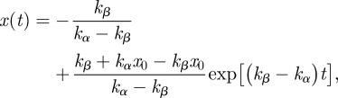2.24

where the initial condition x(t = 0) = x₀ has been used. The calculations for the volume (V)−time dependence are then similar to previously performed calculations and straightforward. After solving equation (2.15) for this special case, V as a function of time equals

2.25

where the initial condition V(t = 0) = V₀ has been used. Equation (2.25) represents a formula for volumetric extension of a cell or non-meristematic tissue axially loaded by the force Mg. As such, it can be useful to the cell growth or wall creep experiments, where the α- and β-expansin proteins may be identified separately. Remarkably, our biochemical model is extremely flexible and can be easily modified to specifically address any given system under consideration.

Now, equipped with equations (2.17)–(2.19), (2.22) and (2.25) derived above, we may proceed to interpretations and applications.

2.2.3. Numerical results

This paper introduces an extension of the Lockhart model that significantly expands the predictive capacities of this equation. Preliminary outcomes of calculations, as described by the equations derived in the preceding paragraphs, are collected in figures 5–9. In order to avoid redundancies and save space, most of the numerical results are described in detail and appear exclusively in the captions coupled to the relevant figures.

Figure 5.

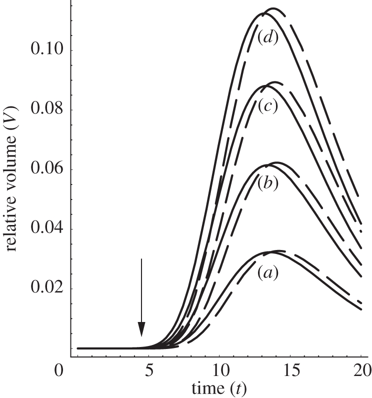
The calculated relative volume V(t) = V_S − V_control under a constant load Mg in the course of time, according to equation (2.17). Expansin action is treated as being proportional to the interacting wall surface area (see the text). (a) S = 1.1, (b) S = 1.2, (c) S = 1.3, (d) S = 1.4. For the intact coleoptile fragments of the same length, we assign S = 1 corresponding to V_control. Plots (a–d) correspond to the solutions of equation (2.17) for the non-abraded fragments (S = 1 is control) subtracted from abraded ones. System response modification owing to the constant uniaxial gravitational force used to induce extension of isolated wall specimens: mass M = 1 (solid lines) and with M = 1.2 (dashed lines). The remaining model parameters (arb. units) are: λ = 2, ω = 1, V₀ = 1, P − Y = 0 and c₁ = c₂ = 1. The arrow indicates the time of expansin application. The reaction kinetics at a constant temperature can be seen, which involves a sharp rise and then the relaxation of an equilibrium process. The plot will change its shape in the descending part when we accept for the control volume, V_control, the linear base line instead of the sigmoid function. A similar remark relates to figures 8 and 9.

Figure 9.

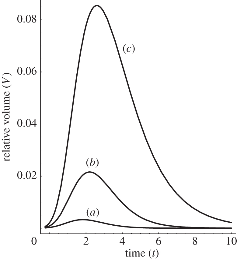
The calculated relative volume, V(t) = V_S − V_control under a constant load Mg in the course of time from equation (2.25). α- and β- expansin protein action is treated as being proportional to the interacting wall surface area (see the text). For the intact coleoptile fragments of the same length, we assign S = 1 corresponding to V_control. Plots (a–c) correspond to the solutions of equation (2.25) for the non-abraded fragments (S = 1 – control) subtracted from abraded ones. System response modification due to the content of α− and β − expansins is presented: (a) k = 0.9, k = 0.1, (b) k = 0.85, k = 0.15, and (c) k = 0.8, k = 0.2. The remaining model parameters (arb. units) are: S = 2, V₀ = 1, x₀ = 1, P − Y = 0 and M = 1.

By way of introduction, we provide some basic solutions. Considering figure 5 (see also the caption), in order to obtain reliable and easy to interpret results, we need to perform a kind of background subtraction of the control volume V_control (t) of an in-abraded fragment (no interaction with exogenous expansin) as it is also usually done in experiment. Consequently, the net area under the relative volume ΔV plots may be identified as equal to the result of expansin action (loosening of plant cell walls caused by expansins, permitting turgor-driven cell enlargement in natural conditions). Thus, we may write the net ‘action’, proportional to the involved intrinsic kinetic processes owing to the expansins from the reservoir (or endogenous), as a definite integral:

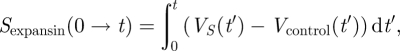2.26

where by V_S we understand the volume change in time under the ‘load + external expansins’, while V_control is understood as the change owing to the ‘load without expansins in the container’ (and, depending on the results of the experiment, the latter may also be reflected by the linear function); t is the time of the experiment duration (time of the interaction of the wall specimen with the expansins from the external reservoir). Even though the explicit analytical formula is accessible by direct substitution of equation (2.17) (also equations (2.18), (2.22) or (2.25)) to the above equation, it can also be retrieved by numerical calculation of cumulative integral of the curves presented in figures 5a–d, 8 (left plot) and 9. As was already mentioned, the area under the curves in figure 5 (and figures 8 and 9) corresponds to the net expansin participation in volumetric expansion (without turgor pressure). Under the assumption of cylindrical geometry of the investigated sample, it is directly proportional to the measured length increment Δl = ΔV/Δr², with r as a specimen (hypocotyl) radius. This also gives a simple empirical method for theory falsification.

Figure 8.

The calculated relative volume, V(t) = V_S − V_control under a constant load Mg in the course of time from equation (2.22). Expansin protein total action is treated as being proportional to the interacting wall surface area (see the text). For the intact coleoptile fragments of the same length, we assign S = 1 corresponding to V_control. Plots (a–c) correspond to the solutions of equation (2.22) for the non-abraded fragments (S = 1 – control) subtracted from abraded ones. System response modification with the initial number n₀ = 10 000 of expansin proteins is presented: (a) k₁ = 0.3, k₂ = 0.2, (b) k₁ = 0.3, k₂ = 0.3, and (c) k₁ = 0.3, k₂ = 0.4. Left chart: Wall creep, with the net turgor pressure, P − Y = 0. Right chart: Vacuolated growth, with P − Y = 0.5 − 0.1 = 0.4. The remaining model parameters (arb. units) are: S = 2, V₀ = 1 and M = 1.

Growing cell walls differ from mature walls in many ways. They are generally thinner, have a different polymer composition and are not highly cross-linked by covalent bonds. They are also pliant and easily deformed by mechanical forces. Such wall pliancy is important for growing cells, because the wall surface must enlarge as the cell grows. The pliancy of growing walls is special in that it enables prolonged wall extension (creep) and stress relaxation. Turgor is required for wall stress relaxation and to provide the driving force to cell growth [38]. The underlying molecular basis for wall pliancy is complex. It seems to be due partly to polymer physics and partly to reactions that alter the bonding relationships of the wall polymers [16]. In this context, the CR can be obtained by calculating the time derivative of the volume V as given by equation (2.17), but with P − Y = 0. The effect can be seen in figure 6 (compare with fig. 5 in [15]). We stress that this solution is not quite a smooth curve but also possesses a characteristic bending at low times, as in the experimental plot (fig. 5 in [15]).

Figure 6.

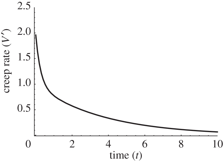
The calculated creep rate, V′ = dV/dt (arb. units) as given by the time derivative of equation (2.17). The model parameters are the same as in figure 5, except M = 0.1; P − Y = 0. Similar plot can be obtained directly for equation (2.19).

An important, and still unresolved, question is the physiological significance of the wall extension studied here. It includes the correlation between CR and long-term GR. Experimental conditions make it difficult to compare ex vivo creep with in vivo growth in a quantitative fashion. It seems that the model equation (2.19) may deliver a proper tool to differentiate both processes and provide a reasonable interpretation (figure 7): at early time points, owing to the high concentration of expansins and consequent weakening of the non-covalent binding between wall polysaccharides, the CR is dominating. Then, after a cross-over, the GR starts to dominate because of the existing turgor pressure and after a maximum is reached, both processes tend to equilibrium. This result is consistent with the experimental results of Schopfer [39], who reported that the initially high CR coefficient slows down continuously with time. With this view, equation (2.19), or the time derivative of equation (2.17), may prove useful in future studies to identify both processes of GR and CR involved.

Figure 7.

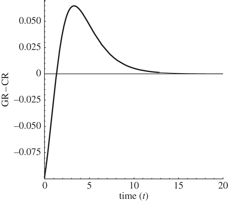
The calculated GR minus CR from equation (2.19). A cross-over from the dominating CR at low times to the dominating GR at greater times is clearly visible. The maximum, due to the turgor pressure, P − Y gradually ceases until the equilibrium is reached. The model parameters are: P − Y = 1 − 0.2 = 0.8 for GR and P − Y = 0 for CR; k₀ = 0.5 in both cases.

2.3. Application to unidirectional stimulus: an anisotropic case

Many experiments in plant physiology are subjected to specific and directional outer perturbations. Equations (2.9) and (2.10) can be used to analyse growth effects caused by a unidirectional stimulus, like the action of collimated light, gravitional field or external pressure. A similar approach has been used to describe spatial auxin redistribution during phototropic response and the connection between light perception and auxin protein carrier's (PIN's) relocation [2]. Also, its applicability to the problems of gravitropic response has also been shown [3]. Based on this experience, there is a hope that further use of equations (2.9) and (2.10) derived in the previous section will provide, as a new mathematical tool, more insight into biological processes where the problem of unilateral stimulus is considered.

3. Discussion

The above derived equation (2.12) can be treated as a new all-purpose dynamic (and thermodynamic) tensor equation of plant cell growth. In particular, it may form an appropriate frame for all observed plant phenomena where the orientation of space matters (this is usually induced by an external unidirectional factor like light or gravity). In this sense, the solution given by equation (2.12) may play a key role in elucidating phototropism and gravitropism. Also, the possible uneven initial concentration of expansin proteins, responsible for cell wall expansion, is represented in equation (2.12) by X (=x₀^ij) matrix.

It is also important to recall that our dualistic solutions (of mechanical and biochemical origin) are obtained by independent reasoning (equations (2.17), (2.18), (2.22) and (2.25)), yet they converge to the same functional that possesses a desirable normalization property:

3.1

This fact is also reflected not only in these global solutions but also in the introduced local solutions—equations (2.9) and (2.10). The convergence to the double-exponent function of all the derived models is a very important property that allows us to compare results and establish empirical relations between different models (parameters) via interpolation to the experimental data. Also, as we see, we are dealing with the upper bound for V(t) corresponding to growth cessation when a cell matures (maximum growth is considered as normalized to unity, and in order to obtain significant results one should always subtract the control value), as opposed to the divergent (exponential) Lockhart solution. Straightforward calculation also yields V(t = 0) = 1/e = 1/2.718 = 0.367, where e stands for the Euler number (this value, if needed, may be subtracted to give V(0) = 0). The calculated double-exponent function [4], V(t) = exp[−exp(−t)], appears to be a good representation of a sigmoid curve able to describe the volumetric growth either by mechanical or biochemical properties. We have also obtained another, even more convenient to use in experimental practice (with the initial volume V₀ normalized to unity: V(t = 0) = V₀ = 1), form of sigmoid-shaped growth functional that appears in calculations, namely:

3.2

It seems that equation (3.2) can be directly applicable as an analytical representation of sigmoidal growth. In fact, growth of any plant organ can be split into three basic phases: the initial phase of slow growth, the intense growth phase and, eventually, the final phase of slow growth. Such regularity can be represented by a sigmoid curve (like equation (3.2); see also fig. 7 in [4]) that characterizes the time course of individual cell growth and the growth of plant organs as a whole [40].

Furthermore, the application of both kinds of equations to experimental data (by standard interpolation) may result in the simultaneous determination of all parameters ((b, k) and k₀ ((k₁, k₂ ) or (k_α, k_β)) from both competing approaches. Consequently, the link between mechanical and biochemical models can be established at a quantitative level. Thus, we can draw further conclusions either on the influence of biochemical parameters (x₀, k₀) ((k₁, k₂), (k_α, k_β)) onto mechanical features (b, k), or, conversely, determine the mechanical properties (b, k) by knowing the biochemical basis.

The sparse set of parameters ((b, k) and k₀ (or (k₁, k₂), (k_α, k_β)), representing, respectively, mechanical and biochemical features of the investigated system, originating from both methods can be determined independently from experimental data (usually obtained in the form of V(t) or V′(t) plots) by interpolation with the help of, e.g., the Levenberg–Marquardt algorithm. Combining both methods may result in the ability to directly analyse biochemical and biomechanical aspects of wall extension itself and finding experimental relations between parameters. Such routine can be performed with data taken directly from the experiment, giving the opportunity to interconnect parameters of both kinds for volumetric plant cell elongation growth or cell wall creep. Thus, we are able to address the problem of fine-tuning of macroscopic mechanical properties using intrinsic biochemical parameters (e.g. kinetic coefficients for α- and β-expansins), and vice versa making at least rough predictions about some biochemical relations by knowing the mechanical features.

The usual experimental routine that can be applied is as follows. First, we need to obtain the volume versus time [V(t)] data (curves) at a given temperature T and fixed pH (usually in a neutral or acidic buffer) under a constant load Mg. The interpolation of measured V(t) points by our final, ready to use equations (equations (2.17), (2.18), (2.22) and (2.25)) will return the values of desired parameters ((b, k), k₀, (k₁, k₂ ) or (k_α, k_β)). These, in turn, may be used to predict the behaviour of V(t) without the need to perform further experiments in different conditions.

As was recently noted [4], the environmental temperature, decisive for growth processes, can be taken into account by the assumption that the kinetic coefficient (k₀) depends on temperature. Such reasoning can be obviously extended to the remaining two-parameter biochemical models proposed in this paper. Let us focus our attention on equation (2.25) derived for volumetric expansion owing to α- and β-expansin protein action. As in the case of the one-parameter model (see also figs 7 and 8 [4]), the effect of temperature on the rates of reaction for a given plant species can be easily established empirically with the help of equation (2.25). By eliminating in separate experiments the influence of α-(or β-) expansins, the empirical values for k_α, k_β coefficients can be determined by interpolation (Levenberg–Marquardt procedure) of the properly modified equation (2.25) to the existing data. Then, the obtained numerical values of k_α, k_β (temperature-dependent) coefficients can be inserted back into equation (2.25) to complete it for further calculations.

Stress relaxation is defined in material science as a reduction in stress at constant strain. As has been shown (eqn (8), Pietruszka [4]), the half-time for stress relaxation (t_1/2) due to expansin action can be compared with Cosgrove's [41] result (eqn (A9), [41]) to give k₀ = ɛΦ₀ that holds at least for t_1/2. This relation combines biochemical (k₀) and biomechanical (ɛ, Φ₀) aspects of plant growth (here ɛ is Young's modulus, which is a measure of stiffness, as in the Ortega [42] equation). Φ₀ takes on the usual interpretation of extensibility coefficient in the Lockhart equation, which is essentially the inverse of viscosity. For many purposes, it is convenient to measure the rate of stress relaxation by a half-time t_1/2, which calculated to give t_1/2 = log 2/k₀ or yields t_1/2 = ɛΦ₀ log 2 when expressed in mechanical terms. However, one of the most interesting results is that the biochemical equation (2.18) may be treated formally (direct calculation) as a consequence of the biomechanical equation (2.17) for λ = ω = k₀. This situation, however, corresponds to the critical damping case, as described quite recently [4], especially applicable for a juvenile cell or organ (the restoring (elastic) term is not present in this case). Therefore, both equations can be applied simultaneously for detailed quantitative analysis emerging from this dual picture.

4. Conclusions

This work is a biologically inspired analysis of expansin enzyme activity on plant cell growth in the anisotropic case. We solve a generalized form of the Lockhart equation and make cell mechanical properties (cell wall extensibility) a time- and space-dependent parameter. This enables us to derive a linear differential equation that accurately models enzymatically mediated relaxation of the polymers composing plant cell walls, thereby allowing pressure-driven polymer creep and plant cell expansion growth.

The equations put forward here to describe cell growth and deformation do have limitations, as they are confined to describing the expansion component of growth. Cell proliferation considerations have not been included here. Also, such semi-phenomenology is not like a microscopic model derived from first principles on the quantum-mechanical level. Moreover, the validity of the presented equations is limited to the non-dissipative temperature region where no membrane leakage takes place. Even though the detailed biochemistry is not discussed here, all the effects are implicit in all functions that account for the effects like enzyme activity, protein synthesis, cell respiration and biomass production. It would be useful to have analytical equations that include a reliable description of cell/organ stretching based on verifiable numbers of mechanical or biochemical origin. In this sense, our model is actually a possible start to a predictive guide for further experimentation.

In spite of all the limitations, the model of expansin action, in which expansins weaken the non-covalent binding between wall polysaccharides, thereby allowing turgor-driven polymer creep, can be successfully described by a linear differential equation of tensors of second order. This model is also consistent with the lack of progressive weakening of the cell wall by expansin and fits well the biophysical characteristics of cell wall extension, the rate of which is dependent on the wall stress P in excess of a minimum yield threshold Y.

On the topic of cell wall growth, most models have traditionally concentrated on one biophysical aspect of growth, namely either on the cell wall extensibility properties or just water pressure-related effects (e.g. hydrostatic pressure, osmotic pressure, turgor threshold). Both components of cell wall growth were usually treated separately and the mutual interactions were not considered or combined into one mathematical model equation. While it seems obvious that both cell wall extensibility properties and water pressure-related effects should be present, simultaneously, in one equation to reflect the self-consistent (e.g. [14]) character of plant cell growth, this has not been thoroughly considered until now. Cell enlargement requires simultaneous water absorption to increase cell volume and irreversible expansion of the cell wall to accommodate the influx of water and to generate a new surface area. Indeed, all environmental agents influencing growth (like stimulators/inhibitors), especially temperature, should be present in the more complete model of cell wall growth. Such an equation should also be susceptible to other modifications, i.e. able to describe phenomena where the direction of the stimulus matters (e.g. phototropism). In this context, we believe that the presented set of (ready to use) growth equations presented here, especially equation (2.12), will be helpful in developing future computation models to reflect quantitatively diverse phenomena observed in plant physiological experiments.

References

- 1.Lockhart A. 1965. An analysis of irreversible plant cell elongation. J. Theor. Biol. 8, 264–275 10.1016/0022-5193(65)90077-9 (doi:10.1016/0022-5193(65)90077-9) [DOI] [PubMed] [Google Scholar]
- 2.Pietruszka M., Lewicka S. 2007. Anisotropic plant growth due to phototropism. J. Math. Biol. 54, 45–55 10.1007/s00285-006-0045-7 (doi:10.1007/s00285-006-0045-7) [DOI] [PubMed] [Google Scholar]
- 3.Lewicka S., Pietruszka M. 2007. Anisotropic plant cell elongation due to ortho-gravitropism. J. Math. Biol. 54, 91–100 10.1007/s00285-006-0049-3 (doi:10.1007/s00285-006-0049-3) [DOI] [PubMed] [Google Scholar]
- 4.Pietruszka M. 2010. Exact analytic solutions for a global equation of plant cell growth. J. Theor. Biol. 264, 457–466 10.1016/j.jtbi.2010.02.012 (doi:10.1016/j.jtbi.2010.02.012) [DOI] [PubMed] [Google Scholar]
- 5.Chen W.-F., Han D.-J. 2007. Plasticity for structural engineers. Fort Lauderdale, FL: J. Ross Publishing [Google Scholar]
- 6.Muller B., et al. 2007. Association of specific expansins with growth in maize leaves is maintained under environmental genetic, and developmental sources of variation. Plant Physiol. 143, 278–290 10.1104/pp.106.087494 (doi:10.1104/pp.106.087494) [DOI] [PMC free article] [PubMed] [Google Scholar]
- 7.Lewicka S., Pietruszka M. 2010. Generalized phenomenological equation of plant growth. Gen. Physiol. Biophys. 29, 95–105 10.4149/gpb_2010_01_95 (doi:10.4149/gpb_2010_01_95) [DOI] [PubMed] [Google Scholar]
- 8.Humphrey T. V., Bonetta D. T., Goring D. R. 2007. Sentinels at the wall: cell wall receptors and sensors. New Phytol. 176, 7–21 10.1111/j.1469-8137.2007.02192.x (doi:10.1111/j.1469-8137.2007.02192.x) [DOI] [PubMed] [Google Scholar]
- 9.Choi D., Cho H.-T., Lee Y. 2006. Expansins: expanding importance in plant growth and development. Physiol. Plant 126, 511–518 [Google Scholar]
- 10.Jones L., McQueen-Mason S. 2004. A role for expansins in dehydration and rehydration of the resurrection plant, Craterostigma plantagineum. FEBS Lett. 559, 61–65 10.1016/S0014-5793(04)00023-7 (doi:10.1016/S0014-5793(04)00023-7) [DOI] [PubMed] [Google Scholar]
- 11.Gao X., Liu K., Lu Y. T. 2010. Specific roles of AtEXPA1 in plant growth and stress adaptation. Russ. J. Plant. Physiol. 57, 241–246 10.1134/S1021443710020111 (doi:10.1134/S1021443710020111) [DOI] [Google Scholar]
- 12.Sabirzhanova I. B., Sabirzhanov B. E., Chemeris A. V., Veselov D. S., Kudoyarova G. R. 2005. Fast changes in expression of expansin gene and leaf extensibility in osmotically stressed maize plants. Plant Physiol. Biochem. 43, 419–422 [DOI] [PubMed] [Google Scholar]
- 13.Xu J., Tian J., Belanger F. C., Huang B. 2007. Identification and characterization of an expansin gene AsEXP1 associated with heat tolerance in C3 Agrostis grass species. J. Exp. Bot. 58, 3789–3796 10.1093/jxb/erm229 (doi:10.1093/jxb/erm229) [DOI] [PubMed] [Google Scholar]
- 14.Pietruszka M. 2009. Self-consistent equation of plant cell growth. Gen. Physiol. Biophys. 28, 340–346 10.4149/gpb_2009_04_340 (doi:10.4149/gpb_2009_04_340) [DOI] [PubMed] [Google Scholar]
- 15.Cosgrove D. J. 1989. Characterization of long-term extension of isolated cell walls from growing cucumber hypocotyls. Planta 177, 121–130 10.1007/BF00392162 (doi:10.1007/BF00392162) [DOI] [PubMed] [Google Scholar]
- 16.Cosgrove D. J. 2000. Loosening of plant cell walls by expansins. Nature 407, 321–326 10.1038/35030000 (doi:10.1038/35030000) [DOI] [PubMed] [Google Scholar]
- 17.Cosgrove D. J. 2005. Growth of the plant cell wall. Nat. Rev. Mol. Cell Biol. 6, 850–861 10.1038/nrm1746 (doi:10.1038/nrm1746) [DOI] [PubMed] [Google Scholar]
- 18.Cho H.-T., Cosgrove D. J. 2000. Altered expression of expansin modulates leaf growth and pedicen abscission in Arabidopsis thaliana. Proc. Natl Acad. Sci. USA 97, 9783–9788 10.1073/pnas.160276997 (doi:10.1073/pnas.160276997) [DOI] [PMC free article] [PubMed] [Google Scholar]
- 19.Cosgrove D. J., Li L. C., Cho H.-T., Hoffmann-Benning S., Moore R. C., Blecker D. 2002. The growing world of expansins. Plant Cell Physiol. 43, 1436–1444 10.1093/pcp/pcf180 (doi:10.1093/pcp/pcf180) [DOI] [PubMed] [Google Scholar]
- 20.Fleming A. J., McQueen-Mason S., Mandel T., Kuhlemeier C. 1997. Induction of leaf primordial by the cell wall protein expansin. Science 276, 1415–1418 10.1126/science.276.5317.1415 (doi:10.1126/science.276.5317.1415) [DOI] [Google Scholar]
- 21.Kwasniewski M., Szarejko I. 2006. Molecular cloning and characterization of α-expansin gene related to root hair formation in barley. Plant Physiol. 141, 1149–1158 10.1104/pp.106.078626 (doi:10.1104/pp.106.078626) [DOI] [PMC free article] [PubMed] [Google Scholar]
- 22.Li X., Xu C., Korban S. S., Chen K. 2010. Regulatory mechanisms of textural changes in ripening fruits. Crit. Rev. Plant. Sci. 29, 222–243 10.1080/07352689.2010.487776 (doi:10.1080/07352689.2010.487776) [DOI] [Google Scholar]
- 23.Lizana X. C., Riegel R., Gomez L. D., Herrera J., Isla A., McQueen-Mason S., Calderini D. F. 2010. Expansins expression is associated with grain size dynamics in wheat (Triticum aestivum L.). J. Exp. Bot. 61, 1147–1157 10.1093/jxb/erp380 (doi:10.1093/jxb/erp380) [DOI] [PMC free article] [PubMed] [Google Scholar]
- 24.McQueen-Mason S., Durachko D. M., Cosgrove D. J. 1992. Two endogenous proteins that induce cell wall expansion in plants. Plant Cell 4, 1425–1433 [DOI] [PMC free article] [PubMed] [Google Scholar]
- 25.Pien S., Wyrzykowska J., McQueen-Mason S., Smart C., Fleming A. 2001. Local expression of expansin induces the entire process of leaf development and modifies leaf shape. Proc. Natl Acad. Sci. USA 98, 11 812–11 817 10.1073/pnas.191380498 (doi:10.1073/pnas.191380498) [DOI] [PMC free article] [PubMed] [Google Scholar]
- 26.Sharova E. I. 2007. Expansins: proteins involved in cell wall softening during plant growth and morphogenesis. Russ. J. Plant. Physiol. 54, 713–727 10.1134/S1021443707060015 (doi:10.1134/S1021443707060015) [DOI] [Google Scholar]
- 27.Sloan J., Backhaus A., Malinowski R., McQueen-Mason S., Fleming A. J. 2009. Phased control of expansin activity during leaf development identifies a sensitivity window for expansin-mediated induction of leaf growth. Plant Physiol. 151, 1844–1854 10.1104/pp.109.144683 (doi:10.1104/pp.109.144683) [DOI] [PMC free article] [PubMed] [Google Scholar]
- 28.Wieczorek K., et al. 2006. Expansins are involved in the formation of nematode-induced syncytia in roots of Arabidopsis thaliana. Plant J. 48, 98–112 10.1111/j.1365-313X.2006.02856.x (doi:10.1111/j.1365-313X.2006.02856.x) [DOI] [PubMed] [Google Scholar]
- 29.Sampedro J., Cosgrove D. J. 2005. The expansin superfamily. Genome Biol. 6, 242 10.1186/gb-2005-6-12-242 (doi:10.1186/gb-2005-6-12-242) [DOI] [PMC free article] [PubMed] [Google Scholar]
- 30.Cosgrove D. J. 1997. Relaxation in a high-stress environment. The molecular basis of extensible walls and cell enlargement. Plant Cell 9, 1031–1041 10.1105/tpc.9.7.1031 (doi:10.1105/tpc.9.7.1031) [DOI] [PMC free article] [PubMed] [Google Scholar]
- 31.McQueen-Mason S., Cosgrove D. J. 1994. Disruption of hydrogen bonding between plant cell wall polymers by proteins that induce wall extension. Proc. Natl Acad. Sci. USA 91, 6574–6578 10.1073/pnas.91.14.6574 (doi:10.1073/pnas.91.14.6574) [DOI] [PMC free article] [PubMed] [Google Scholar]
- 32.McQueen-Mason S., Cosgrove D. J. 1995. Expansin mode of action on cell walls. Plant Physiol. 107, 87–100 [DOI] [PMC free article] [PubMed] [Google Scholar]
- 33.Takahashi K., Hirata S., Kido N., Katou K. 2006. Wall-yielding properties of cell walls from elongating cucumber hypotcotyls in relation to the action of expansins. Plant Cell Physiol. 47, 1520–1529 10.1093/pcp/pcl017 (doi:10.1093/pcp/pcl017) [DOI] [PubMed] [Google Scholar]
- 34.Wang C. X., Wang L., McQueen-Mason S., Pritchard J., Thomas C. R. 2008. pH and expansin action on single suspension-cultured tomato (Lycopersicon esculentum) cells. J. Plant Res. 121, 527–534 10.1007/s10265-008-0176-6 (doi:10.1007/s10265-008-0176-6) [DOI] [PubMed] [Google Scholar]
- 35.Sasayana D., Azuma T., Itoh K. 2009. Changes in expansin activity and cell wall susceptibility to expansin action during cessation of internodal elongation in floating rice. Plant Growth Regul. 57, 79–88 10.1007/s10725-008-9325-0 (doi:10.1007/s10725-008-9325-0) [DOI] [Google Scholar]
- 36.Kapu N. U. S., Cosgrove D. J. 2010. Changes in growth and cell wall extensibility of maize silks following pollination. J. Exp. Bot. 61, 4095–4107 10.1093/jxb/erq225 (doi:10.1093/jxb/erq225) [DOI] [PMC free article] [PubMed] [Google Scholar]
- 37.Okamoto-Nakazato A., Takahashi K., Katoh-Semba R. 2002. Distribution of yieldin, a regulatory protein of the cell wall yield threshold, in etiolated cowpea seedlings. Plant Cell Biol. 42, 952–958 [DOI] [PubMed] [Google Scholar]
- 38.Cosgrove D. J. 1987. Wall relaxation in growing stems: comparison of four species and assessment of measurement techniques. Planta 171, 266–278 10.1007/BF00391104 (doi:10.1007/BF00391104) [DOI] [PubMed] [Google Scholar]
- 39.Schopfer P. 2001. Hydroxyl radical-induced cell-wall loosening in vitro and in vivo: implications for the control of elongation growth. Plant J. 28, 679–688 10.1046/j.1365-313x.2001.01187.x (doi:10.1046/j.1365-313x.2001.01187.x) [DOI] [PubMed] [Google Scholar]
- 40.Fogg G. E. 1975. The growth of plants. Suffolk, UK: Richard Clay (The Chaucer Press) [Google Scholar]
- 41.Cosgrove D. J. 1985. Cell wall yield properties of growing tissue. Plant Physiol. 78, 347–356 10.1104/pp.78.2.347 (doi:10.1104/pp.78.2.347) [DOI] [PMC free article] [PubMed] [Google Scholar]
- 42.Ortega J. K. E. 1985. Augmented growth equation for cell wall expansion. Plant Physiol. 79, 318–320 10.1104/pp.79.1.318 (doi:10.1104/pp.79.1.318) [DOI] [PMC free article] [PubMed] [Google Scholar]