Modelling the initial phase of an epidemic using incidence and infection network data: 2009 H1N1 pandemic in Israel as a case study

Abstract

This paper presents new computational and modelling tools for studying the dynamics of an epidemic in its initial stages that use both available incidence time series and data describing the population's infection network structure. The work is motivated by data collected at the beginning of the H1N1 pandemic outbreak in Israel in the summer of 2009. We formulated a new discrete-time stochastic epidemic SIR (susceptible-infected-recovered) model that explicitly takes into account the disease's specific generation-time distribution and the intrinsic demographic stochasticity inherent to the infection process. Moreover, in contrast with many other modelling approaches, the model allows direct analytical derivation of estimates for the effective reproductive number (R_e) and of their credible intervals, by maximum likelihood and Bayesian methods. The basic model can be extended to include age–class structure, and a maximum likelihood methodology allows us to estimate the model's next-generation matrix by combining two types of data: (i) the incidence series of each age group, and (ii) infection network data that provide partial information of ‘who-infected-who’. Unlike other approaches for estimating the next-generation matrix, the method developed here does not require making a priori assumptions about the structure of the next-generation matrix. We show, using a simulation study, that even a relatively small amount of information about the infection network greatly improves the accuracy of estimation of the next-generation matrix. The method is applied in practice to estimate the next-generation matrix from the Israeli H1N1 pandemic data. The tools developed here should be of practical importance for future investigations of epidemics during their initial stages. However, they require the availability of data which represent a random sample of the real epidemic process. We discuss the conditions under which reporting rates may or may not influence our estimated quantities and the effects of bias.

1. Introduction

In the early stages of an epidemic, there is urgency in assessing the potential magnitude, severity and rate of spread over geographical regions and in different sub-populations so that rapid and appropriate policy schemes can be formulated [1–3]. Such complex assessments have to be made under great uncertainty due to the lack of data available and the fact that they are often of poor quality [4]. Mathematical models are an effective tool for investigating the dynamics of the spread of epidemics, including possible control strategies, but in order to apply a model to a particular situation there is a need to be confident that the values used for the various parameters in the model correspond to reality. While some parameters can be determined based on previous knowledge, other parameters must be estimated by fitting the model to the available data. Thus, fitting epidemiological models to real data becomes a central problem for the field of infectious disease epidemiology.

In this work, we describe new epidemic models and methods for fitting these models to the different types of data that can be collected at the initial stages of an epidemic. These tools were developed for the purpose of analysing data collected during the first weeks of the spread of the 2009 A/H1N1 influenza pandemic in Israel. The methods and their application to the Israeli H1N1 data are the main focus of this paper. It is our hope that these methods will be useful for analysing future epidemics in their initial stages.

During the first two months of the 2009 A/H1N1 influenza outbreak in Israel (from 26 April 2009 until 7 July 2009) the national health authorities in Israel attempted to identify and test all cases of people suspected with symptomatic influenza. Their efforts were aided by the high media impact of the disease and the attentiveness of the general public. There is reason to believe that nearly all influenza-like illness cases in Israel over this period were tested in the national surveillance campaign (see [5] for further analysis of this dataset). During the time span in which our data were collected, the number of laboratory-confirmed cases in Israel (713) was the third highest in Europe, exceeded only by the UK and Spain, which have much larger populations [6]. The national surveillance also provided infection network data, i.e. partial information regarding ‘who-infected-who’. Our work aimed at extracting as much information as possible from the available data.

The analyses are based on a new discrete-time stochastic epidemic model. The equations used are closely related to the well-known SIR epidemic model [7–10]. However, our ‘age-of-infection’ model explicitly takes into account the disease's specific generation-time distribution. This contrasts with the unrealistic default (exponential) distribution of the standard SIR model. The model we present also allows for intrinsic demographic stochasticity that is inherent in the infection process, and in a simplified manner that makes it possible to rapidly generate large numbers of simulations. However, the most important advantage of the model is that it allows an analytical derivation of parameter estimates by maximum likelihood and by Bayesian methods. The model thus provides a powerful framework for analysis of epidemics in general.

In §2, we describe the basic version of the discrete age-of-infection model which posits a homogeneous population. We formulate a maximum likelihood approach for fitting the model to incidence data that yields analytical estimates for the effective reproductive number R_e. The approach also permits estimation of Bayesian credible intervals for R_e, and bootstrap confidence intervals (CIs) are also computed using simulations. The modelling methods are then used to fit the Israeli dataset to obtain estimates for R_e during the H1N1 pandemic in its initial stage.

In §3, we consider a more elaborate version of the model in which the population is divided into different age groups. Using a simulation study, we demonstrate that in this case, fitting the model using incidence data for each age group fails to provide accurate parameter estimates for realistic sample sizes. In view of this, a new maximum likelihood approach is developed that estimates the parameters of the age group model using a combination of two types of data: the incidence data and infection network data. The power of combining the two datasets is demonstrated using a simulation study, showing that the who-infected-who data significantly increases the accuracy of estimates of the model parameters. The method is then applied to the Israeli dataset, yielding estimates of the ‘next-generation matrix’ for the spread of the H1N1 pandemic among three age groups.

1.1. Data

The data studied here consist of laboratory-confirmed cases of individuals infected with 2009 H1N1 influenza. The first person in Israel diagnosed as suffering from novel H1N1 infection arrived in Israel from Mexico, and was hospitalized in the Laniado hospital on 26 April 2009. A database of cases was assembled at the Central Virology Laboratory, Tel-Hashomer, Israel, for the period 26 April to 7 July 2009. In this 10 week period, altogether ca 2400 samples of patients with symptoms of influenza-like illness (IL) were tested, of which 713 (30%) were found positive for the novel strain. The Israeli Ministry of Health and Center for Disease Control has argued that this number should closely match all Israelis with symptomatic novel H1N1 influenza in this time period. As a result of the WHO guidelines, the systematic collection of samples from all suspected patients ended after 2 July 2009. Therefore, when estimating model parameters we use 2 July as the end date, in order to avoid biases due to differences in sampling effort. While constructing the database various characteristics for each patient were also recorded, including sex, age, geographical locality, examination date and whether the patient had arrived on a flight to Israel during the week prior to the examination. In addition, individuals tested were asked by their doctor whether they could identify the person from whom they believed they were infected.

In this paper we used the following data extracted from the above database:

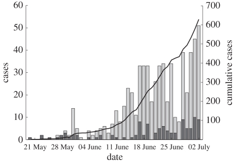
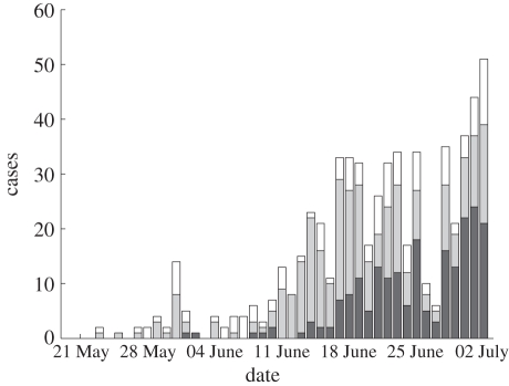
• — Incidence data. The time series of all 2009 H1N1 influenza cases in Israel during the initial phase of the outbreak is displayed in figure 1. Infected individuals, who had arrived from abroad during the week prior to their examination, were classified as imported cases and the remainder were classified as local cases. As can be seen from figure 1, at the beginning of the period, only sporadic imported cases were recorded. Only from 20 May and onwards, did the epidemic start to spread in the Israeli population. In our analysis, we therefore used the incidence data of the period from 20 May to 2 July 2009, with a total of 629 cases. For the purpose of our age group model, we divided all cases into three different age groups 0–18, 19–29 and 30 and above, describing children, young adults and adults. Of the 629 cases between 20 May and 2 July 2009, there were 616 cases with records available for the age group analysis. Figure 2 shows the time series of all cases divided into the three age groups. Given that the number of cases for age 30+ is far fewer than cases between the ages 19 and 29, it was decided to divide the adults into two groups.

• — Infection networks. The information provided by some infected patients made it possible to construct infection networks which map the connections between an infected person (infector) and the individuals he or she infected (infectees). Links were established either

  1. when an infectee was able to identify a particular patient in the database as the infector (65 links), or
  2. based on circumstantial evidence (58 links) as to when the patient reported that his/her infection occurred in a school class, from a neighbour, etc. This, in many cases, provided information that identified another patient in the database who was most probably the infector.

Out of a total of 123 infection links, there were 97 links between 20 May and 2 July for which we had the age of both the infector and the infectee.

• — Generation-time distribution. Based on the infection networks, it was possible to estimate the generation-time interval distribution for the 2009 H1N1 influenza. This is the distribution of the durations between the time an individual becomes infected and the times of infection of the people he or she infects. Since the infection time is not known, we used the durations between reported disease initiations as estimates for the generation-time intervals. Out of the 123 connections in the infection networks, 54 connections had specified disease initiation dates at both ends of the link, with the differences between the two dates ranging from 0 to 15 days. The mean generation time was found to be μ = 2.92 and its standard deviation σ = 1.79 based on a generation-time distribution of up to 7 days. We limited our data to intervals of up to 7 days since longer intervals are considered controversial [11]. For more details see [5].

Figure 1.

Confirmed 2009 H1N1 influenza cases in Israel between 20 May 2009 and 2 July 2009, altogether 629 cases. Bars represent the incidences per day (left y-scale), and contain both imported (dark grey region) and local (light grey region) cases. The solid line indicates the cumulative number of cases (right y-scale).

Figure 2.

Confirmed 2009 H1N1 influenza cases in Israel between 20 May 2009 and 2 July 2009 divided into three age groups 0–18 (209 cases, dark grey region), 19–29 (280 cases, light grey region), 30+ (127 cases, white region).

2. Discrete time stochastic age-of-infection model and estimation of r_e

2.1. Discrete time stochastic age-of-infection model

For a population of N individuals, we denote the number of newly infected individuals on day t by i(t) and let S(t) be the number of susceptibles at the end of day t. i⁰(t) is the number of imported infectives on day t. The model equations, which are derived below, are a Poisson approximation of a generalization of the classical chain binomial SIR model and may be written as,

2.1a

and

2.1b

Here Poisson(x) is a random variable having a Poisson distribution of mean x, which accounts for demographic stochasticity (see the derivation below). The reproductive number R₀ defines the average number of people infected by a typical individual over his/her infectivity period in a totally susceptible population.

In this model formulation, infected individuals are assumed to remain infected for a maximum of up to d days, where, unless otherwise stated, d = 7 [11]. It is thus related to age-of-infection epidemic models [7,12], but in a discrete rather than continuous form. The numbers P_τ (1 ≤ τ ≤ d) represent the generation-time distribution; in a totally susceptible population, P_τ is the fraction of infections generated by an infective person which occur on day τ of infection (thus ). It should be noted that since this model allows a general generation-time distribution, in particular admitting a latent period of l days described by taking P_τ = 0 for 1 ≤ τ ≤ l < d, it subsumes models such as the SEIR model. Estimates of the generation-time distribution P_τ for the 2009 novel H1N1 epidemic were derived from the infection networks data as described in §1.1. As imported infectors arriving from abroad formed a substantial proportion of the infected subpopulation in the early phase of the epidemic, it proved essential to incorporate them realistically into the model equations, and we noted (see §4) that our main results were sensitive to their presence. The procedure we use for generating realizations of the stochastic model is as follows. At each time step we draw the number of new infectives i(t) according to the Poisson distribution given in equation (2.1a). This requires knowledge of the numbers of immigrant infectives i⁰(t) which are available from our surveillance data. Then the susceptible numbers S(t) are updated according to equation (2.1b).

The model is derived as follows. Let m denote the average number of contacts per individual per day and let N denote the total population size. Define p_τ (1 ≤ τ ≤ d) as the infectivity profile for the d days of infection, that is p_τ is the probability that a contact between a susceptible and an infective, whose age of infection is τ days, results in infection of the susceptible. Suppose we are now on day t, and consider an infective person who was infected τ days ago. This individual meets each other individual with probability (m/N), so that he/she infects each susceptible with probability (m/N)p_τ. Therefore, the number of susceptibles infected by this infective is binomially distributed with parameters n = S(t − 1) and p = (m/N)p_τ. Since m ≪ N, we have p ≪ 1, np = mp_τS(t − 1)/N, so that the Poisson approximation to the binomial distribution is valid and we may assume that the number of people infected by an infective on day t is Poisson distributed with mean mp_τS(t − 1)/N. Therefore, the number of people infected on day t by all infectives with age-of-infection τ is Poisson distributed with mean mp_τ(S(t − 1)/N)[i(t − τ) + i⁰(t − τ)], and summing over 1 ≤ τ ≤ d we obtain

2.2

Note that, since an infective placed in a totally susceptible population would infect mp_τ people on the τth day of infectivity, the total number of infections that an infective would produce, that is the basic reproduction number, is given by . Therefore, setting we can rewrite equation (2.2) as equations (2.1a,b). The numbers P_τ represent the generation-time distribution: P_τ is the fraction of the infections generated by a person which occur on the τth day of infection.

Since we are dealing with the initial phase of the epidemic, the depletion of susceptibles is negligible (S₀ is of the order of millions and only a few hundred cases are depleted) and the model may be simplified by setting S(t) = S₀, obtaining

2.3

where R_e is the effective reproductive number, given by R_e = (S₀/N)R₀.

At the beginning of an epidemic, results from the ‘linearized’ model (2.3) are virtually identical with those obtained from the ‘full’ model (2.1), and only at much later stages of the epidemic, when a significant fraction of the susceptibles becomes depleted, does it become important to use the full model. Therefore, our analysis in this paper employs equation (2.3).

2.2. Estimating the effective reproductive number

It is clear from the form of the model (2.3) that R₀ and S₀ are not separately identifiable. For a pandemic involving a new pathogen it is sometimes assumed that S₀ = N (no immunity in the population), so that R₀ = R_e. However, in the case of the 2009 H1N1 influenza, there was indication of partial immunity among older people [13]. In this paper, we make no claim about R₀ and estimate only R_e.

In the following, we derive a maximum likelihood estimate for R_e. The likelihood function, that is the probability of obtaining the data i(t) (1 ≤ t ≤ T), where T is the number of days of data available from model (2.3), is given by

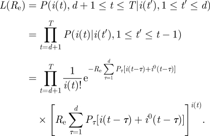Defining the log-likelihood LL(R_e) = log(L(R_e)) and differentiating with respect to R_e we obtain

so that the maximum likelihood estimator for R_e is given by

2.4

We note that, except for the inclusion of the imported infectives, this estimator is the same as the one derived by White & Paganno [14]. We note however that White & Pagano's derivation of the maximum likelihood function was achieved using a quite different approach based on branching process considerations that describe an infection process. We believe that the derivation of the estimator (2.4) from an explicit SIR dynamical model simplifies the argument. In [15] a similar estimator was used to estimate the reproductive number of 2009 H1N1 in the USA, and the imported infectives were included in a way that is equivalent to that in estimator (2.4) above. In view of the fact that this estimator is a maximum likelihood estimator for a model which incorporates the generation-time distribution and stochasticity, it offers a very attractive and more direct alternative to the widely applied approach for estimating R_e based on estimating the exponential growth rate r of the epidemic curve and relating r to R_e using the generation-interval distribution [16].

We propose two methods to obtain an interval estimate for R_e, in addition to the point-estimate :

• — Bootstrap CI. Generate 1000 simulated epidemics using the model (2.3) with (as estimated from the data using formula (2.4)) and the observed imported infectors i⁰(t), obtaining 1000 incidence series i(t). For each of these simulated epidemics re-estimate R_e using formula (2.4) and remove the 25 lowest and 25 highest estimates to obtain a 95% bootstrap CI for R_e.

• — Bayesian credible intervals. The likelihood approach allows the derivation of Bayesian 95% CI (see appendix for details) given by , where

  

2.3. Application to Israeli H1N1 2009 pandemic data: estimation of R_e

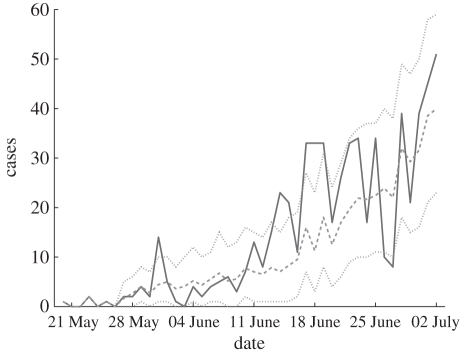
For the Israeli 2009 H1N1 influenza time series, our modelling approach (formula (2.4)) produced estimates of R_e≈1.06 with a 95% bootstrap CI [0.97,1.16]. The Bayesian 95% CI is nearly identical. Figure 3 displays the observed H1N1 incidence series, the incidence series obtained by averaging 1000 simulations of the stochastic model (2.3) with our estimate of R_e, and bands containing 95 per cent of the values of these simulations. The observed curve deviates only slightly outside the 95 per cent bands of the fitted model, which might suggest that there is some process that the model does not fully capture. This issue will be further discussed in the §3, in relation to the age group model.

Figure 3.

Confirmed 2009 H1N1 cases (solid line), with the simulation curve obtained by averaging 1000 simulations of the stochastic model (2.2) using the estimated R_e (dashed line), together with 95% bands (dotted lines).

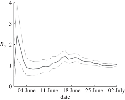
We tested how the prediction of R_e and its Bayesian 95% CI change with respect to changing the time span used in the calculation. This allows us to examine the question: how far into the epidemic do we have to be before a reasonably accurate estimate of R_e can be obtained? Figure 4 displays how R_e and its Bayesian 95 per cent credible intervals change with respect to changing the time span used in the calculation. The graph shows estimations for R_e based on the observation periods initiating on 20 May and ending on each day between 30 May and 2 July. The credible intervals narrow significantly as the observation period increases. After about a month of data, the estimate of R_e is sufficiently accurate so that the uncertainty as measured by the 95% CI is reduced to ±10 per cent of the estimated value.

Figure 4.

Changes in R_e estimates as the epidemic progresses. For each day, starting from 30 May, R_e is estimated based on the time series initiating on 20 May up to that day. The solid line depicts the estimated R_e values and the dashed lines the 95% Bayesian lower and upper credibility intervals.

Various estimates of the reproductive number have been made for the initial phase of the epidemic in different regions of the world [15,17–26]. These estimates range from 0.5 to 3.4 [17,27]. However, most lie in the 1.2–1.6 range, and very few are lower than this range. Thus our estimate of R_e = 1.06 for Israel is indeed relatively low. The estimates we obtained are also lower than estimates based on data from previous pandemics [28].

There are several factors that can explain differences in R_e = R₀S₀/N estimated at different locations worldwide. Local variation in either the basic reproductive number R₀ or the percentage of the susceptible population S₀ can lead to differences in R_e values. Since climactic conditions are believed to play a role in the low transmissibility of flu during the summer, variations in climate in different locations may lead to different R₀. An alternative explanation is that the Israeli population has more immunity (i.e. lower S₀) to the pandemic virus, possibly due to greater cross immunity to seasonal H1N1, compared with Mexico for instance. Many studies assume that all, or most, of the population are susceptible to pandemic influenza. Today there is accumulating evidence that the population immunity for pandemic strains cannot be neglected and can vary considerably between different locations [13,29]. Another possible explanation is that the Israeli authorities' containment measures were more efficient than in other regions and hampered faster epidemic spread, resulting in a low R_e. Finally, we have noted that, when estimating R_e in the initial phase of an epidemic, taking the imported infectives into account in an appropriate way (as in formula (2.4)) is important, and that not doing so will lead to an upwardly biased estimate of R_e (see §4). It is possible that some of the estimates in the literature that were obtained at the beginning of the epidemic are too high because imported infectives were not taken into account separately.

It should be stressed that the low estimated value of R_e relates to the specific period of time in which the data were collected during the summer season. Since it is generally believed that the transmission rate of influenza varies with the season of the year [30], it was expected that the reproductive number would increase during the autumn and winter.

3. Discrete time stochastic age-of-infection model with age groups and estimation of the next-generation matrix

3.1. The stochastic age-of-infection model with age groups

The model described in the previous section neglects the effects of heterogeneity in the population. Here we expand this model by dividing the population into n age groups which can have different characteristics. In an age group model, the ‘next-generation matrix’ β encodes the contact structure among different age groups, as well their differential susceptibility and infectivity. The matrix element β_jk represents the expected number of secondary infections in age group j due to a single primary infection in age group k [7,29]. If the matrix β is estimated at the beginning of the epidemic, it may be used to predict the further unfolding of the epidemic as well as to help plan an optimal vaccination and mitigation strategy [31]. Using the matrix β, we generalize the model (2.3) to n age groups. We denote the number of locally infected new infectives in the jth age group on day t by i_j(t), and the number of imported infectives in age group j arriving on day t by . We also denote the number of locally infected new infectives in the jth age group who were infected by individuals from age group k on day t by i_jk(t), so that

3.1

The model is thus

3.2

Hence by equation (3.1)

3.3

where, as before, p_τ (1 ≤ τ ≤ d) is the generation-time distribution.

Note that in the case n = 1 equation (3.3) reduces to (2.3), with β₁₁ = R_e, so that the multi-group model generalizes the homogeneous-population model considered in §2.

Our aim is to use the available data in order to estimate the next-generation matrix β. In general, estimating the matrix β based on incidence time series for each of the groups is difficult, due to the large number of parameters (n²). Efforts in the literature to address this problem attempt to reduce the number of parameters that need to be estimated. One such method restricts the structure of the matrix β in certain ways, for example by assuming proportionate mixing, or assuming that certain groups of matrix elements are equal [32–34]. Another approach is to use independent data drawn from surveys on social contacts between people in various age groups [35].

Here, we develop a new approach that exploits the fact that we have, in addition to the incidence data, a dataset consisting of infected individuals for whom we know the identity of the individual who infected them, and in particular the age groups to which the infector and the infectee belong are known. These data contain information on the next-generation matrix β. To extract this information, a likelihood function is formulated, which expresses the probability of obtaining the two types of data (incidence data and infection network data) as a function of the matrix β. The likelihood function is then maximized with respect to the matrix parameter β, resulting in the maximum likelihood estimate for β. We now describe the construction of the likelihood function.

3.2. Derivation of the likelihood function

Our two types of data available are thus:

• (D_I) Incidence data. The numbers i_j(t), of new local and imported cases in group j for 1 ≤ j ≤ n, 1 ≤ t ≤ T.

• (D_II) Infection network data. A set of L triples (t_l, j_l, k_l) (1 ≤ l ≤ L), where (t_l, j_l, k_l) indicates that on day t_l a member of group j_l was infected by member of group k_l.

Assuming now that the infection process is described by the model (3.3), we compute the probability L(β) = P(D_I, D_II|β), which can be decomposed as

3.4

Each of the terms in the decomposition (3.4) may be computed separately. The quantity P(D_I | β), that is the probability of obtaining the incidence data i_j(t) from model (3.3) given knowledge of β, is a direct generalization of the computation made above for the one-group model, giving

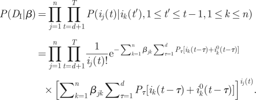3.5

Next we compute P(D_II|β, D_I), which is the probability of obtaining the data (t_l, j_l, k_l) (1 ≤ l ≤ L) given the knowledge of β and of the incidence data i_j(t). Assume that we randomly sample a member of group j who was locally infected on day t. We will compute the probability P((t,j,k)|β, D_I) that the infector of the sampled individual is in group k. The likelihood of obtaining the dataset (t_l, j_l, k_l) (1 ≤ l ≤ L) is then given by

3.6

It should be noted that the above makes no assumption about the manner in which the infected cases whose infector is known are drawn from the population. In particular, the probability of an infected person being asked about or being aware of the identity of their infector is not assumed to be independent of the age of the infected person. The probability computed is that of an individual's infector being in a certain age group k conditional on the assumption that the infected individual is in a certain age group j.

Given knowledge of i_jk(t) (the number of people from group j who were infected by a member of group k), the probability that the infector of a random member of group j is a member of group k is simply P((t,j,k)|D_I, i_jk(t)) = i_jk(t)/i_j(t). However, we do not know the value of i_jk(t) (in other words, it is a latent variable), but we can compute the probability distribution of i_jk(t) given β and D_I, as done below. Thus, given the values of β and of the incidence data D_I, the probability P((t,j,k)|D_I, β) will be computed as

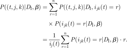3.7

We need, then, to compute P(i_jk (t) = r|D_I, β). To do so, it is convenient to set X = i_jk(t), and note that, by equation (3.1), the value

3.8

is known, given D_I. Also, by equation (3.2), we have that

3.9

We now note the following general fact: if X and Y are independent random variables with X ∼ Poisson(a) and Y ∼ Poisson(b), then the distribution of X given that it is known that X + Y = m, is binomial, given by

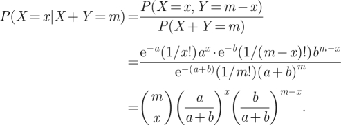Applying this to our X and Y, using equations (3.8) and (3.9) we obtain

where

Therefore, from equation (3.7)

and together with equation (3.6) we obtain

3.10

Combining equations (3.4), (3.5) and (3.10) we finally have our likelihood function.

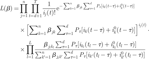3.11

We used the numerical routine fminunc in Matlab (Mathworks) to maximize this function with respect to the parameters β_jk.

3.3. Testing performance on simulated data

A simulation study was conducted to test the performance of this maximum likelihood procedure for estimating β, and in particular to examine whether the information contained in a dataset of the size that we have is sufficient for obtaining accurate estimates of the parameters. Simulated data D_I and D_II were generated using a matrix β that we chose in advance. These data were used to estimate the matrix by maximizing the likelihood (3.11), obtaining an estimated matrix , which was then compared with the true β generating the data.

The simulated data D_I and D_II are generated as follows:

• — Starting with some initial values i_j(t) for days 1 ≤ t ≤ d, we simulate, for each day d + 1 ≤ t ≤ T, the number i_jk(t) of people in age group j who were infected on that day by people in age group k, and the total number of infected individuals in age group j. This requires randomly drawing i_jk(t) according to

  

  (we took , the number of imported cases, to be zero in our simulations).

• — For each 1 ≤ l ≤ L, we randomly uniformly choose a day d + 1 ≤ t_l ≤ T and a group 1 ≤ j_l ≤ n, and then choose 1 ≤ k_l ≤ n (the age group of the infector of an individual in group j_l who was infected on day t_l) at random with the probabilities

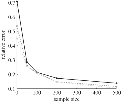
In the simulation tests, we took n = 3 age groups, and arbitrary matrices β were chosen. The quality of estimation was determined for different amounts of simulated data, by varying the number of days T used (and hence the number of cases in the incidence series) and the size L of the available infection network. For each value of L and T, 100 sets of simulated data D_I and D_II were generated. For each of these the estimated matrix was computed using the maximum likelihood method described above, and the relative error

3.12

where the norm of a matrix M is given by was computed. The average relative error over the 100 simulated datasets is reported.

Figure 5 shows the results from one typical example. As expected, the quality of the estimate increases both with the number of days of incidence data and with the size of the infection network available. Especially significant is the comparison of the quality of the estimate for L = 0 (i.e. no infection network data and β is estimated based only on the time series of infectives), to the case where a small amount (L = 50) of infection network data are available. We see a dramatic improvement in the accuracy of the estimation, even with a small amount of infection network data. For example, 30 days into the epidemic, estimating β on the basis of incidence data alone would given an average relative error of RE = 0.8, which means that the estimate is worthless, but with only L = 50 cases in the infection network data a relative error of RE = 0.29 is obtained, indicating a dramatic improvement.

Figure 5.

Simulation study of estimation of the next-generation matrix β using our maximum likelihood method. Generating simulated data using the matrix (with dominant eigenvalue R₀ ≈ 1.4), our method was used to estimate β from the simulated data. The relative error, given by equation (3.12), for the next-generation matrix estimation for various values of L (number of who-infected-who samples) and T (number of days of incidence data), is shown (filled black circle, T = 30; filled inverted triangle, T = 45; filled grey squares, T = 60).

3.4. Bootstrap CIs for the next-generation matrix

To quantify the precision of our estimate of the next-generation matrix, bootstrap CIs were constructed using a procedure similar to the one used in the simulation tests discussed in §3.3. After obtaining the estimate , 1000 realizations of the data D_I and D_II were simulated, using as the next-generation matrix, with T = 44, L = 97 matching the observed data, and with numbers of imported cased taken from the observed data. For each of these 1000 datasets, the next-generation matrix was re-estimated, yielding 1000 matrices . For each component of this matrix, the highest and the lowest 25 values were removed. The interval containing the remaining values gives, for each component, the 95% bootstrap CI.

3.5. Estimation of the next-generation matrix for the Israeli H1N1 pandemic data

For our data on confirmed cases from the initial period of the H1N1 pandemic in Israel in the summer of 2009, we used incidence data from three age groups (0–18, 19–29, 30+), with T = 44 days (20 May–2 July), and infection network data with L = 97 infectees. We also made use of , the number of imported cases in each age group, from our data. The resulting maximum-likelihood estimate , together with the 95% bootstrap CIs calculated as described in §3.4, were found to be

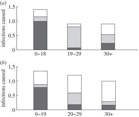
This means, for example, that a child (0–18) infects, on average, 0.99 children, 0.16 young adults (19–29) and 0.25 adults (30+). The information contained in this matrix is displayed in figure 6a. The height of each column in the figure represents the average number of individuals that one person in the corresponding age group infects, and each column is divided into three parts representing the number of infections in each age group. The spectral radius of is , slightly higher than what was found using the homogeneous model.

Figure 6.

(a) Representation of the estimated next-generation matrix β: each bar represents the average number of infections caused by a single infected individual of the corresponding age group in each of the age groups. (b) Representation of the next-generation matrix based only on social contacts as derived from the POLYMOD study [37]. The ages are grouped slightly differently than in (a) since the social contact matrices in this study were given in 5-year age bands (filled dark grey region, 0–18; filled grey region, 19–29; white region, 30+).

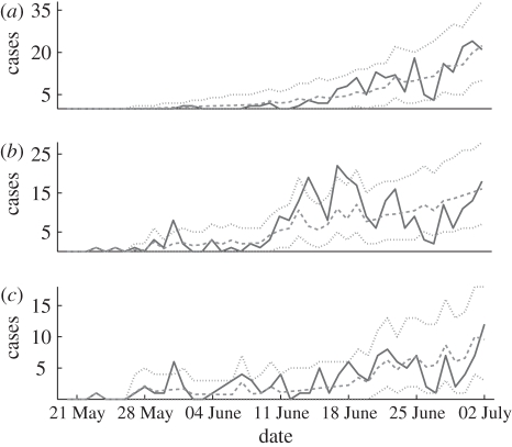
To test goodness of fit, figure 7 displays the incidence time series in each of the three age groups, together with 95 per cent bands for the incidences, generated by 1000 simulations according to model (3.3), using the estimated matrix . While the incidences for the children and adult groups always lie within the 95 per cent band obtained from simulation, for the young adult group we find some deviations from this band on certain days. In other words, the fitted three age group model does not completely capture the epidemic dynamics. This can be due to some heterogeneity which is not taken into account by the model. More particularly, we hypothesize that infections among army soldiers, who are part of the young adult group, may play a role here, as the contact patterns of soldiers are likely to differ from those of other young adults.

Figure 7.

Confirmed 2009 H1N1 cases in each age group (solid line) and the simulation curve obtained by averaging 1000 simulations of the stochastic age group model (3.3) using the estimated matrix β (dashed line), together with 95% bands (dotted lines). (a) 0–18 age group, (b) 19–29 age group and (c) 30+ age group.

It is of interest to compare the estimated next-generation matrix with the matrix that would be obtained based on data about contacts among individuals of different age groups. According to the ‘social contact hypothesis’ [35,36], variations in epidemic dynamics in different age groups can be explained by the different contact rates among different groups. Since data on social contacts in Israel are not available, we employ data from the European POLYMOD study [37]. The matrices corresponding to eight European countries were averaged, and age groups were aggregated to obtain a 3 × 3 matrix corresponding as closely as possible to the age groups considered here. The resulting matrix was multiplied by a constant so as to obtain a matrix with a dominant eigenvalue of 1.14, identical to that of the estimated matrix . The result is presented in figure 6b. We observe considerable differences between the matrix estimated from our data and the European contact matrix. The most significant difference is that according to our estimated matrix , the number of members of the 30+ age group that are infected by members of each of the age groups is much lower than would be expected from the European contact matrix. In other words, the relatively low incidence rate in the adult age group cannot be accounted for solely in terms of social contacts, at least under the assumption that the European contact matrix reflects social contacts in Israel. This supports the hypothesis of reduced susceptibility of people in the 30+ age groups, compared with younger age groups as was suggested by other studies [38,39].

4. Discussion

The modelling tools and analyses that have been described here could be valuable in real time to help obtain a picture of the unfolding of an epidemic during its onset phase. They rely on: (i) credible daily incidence data, including classification of cases into ‘imported’ versus ‘local’ infections, (ii) representative sampling of infection networks. We now discuss several general points, which we found to be of importance and could be significant for future work in analysing epidemics.

In the case study reported here we were fortunate to possess an excellent database, due to the fact that at the beginning of novel H1N1 epidemic strong efforts were taken by the Israeli health authorities to test every suspected case of influenza. It should be noted, however, that the application of the methods presented here does not require that the available incidence data be complete, so that they can be employed in contexts where detection is far from complete. For example, since the estimator (2.4) for the effective reproductive number is invariant to multiplication of all the values i(t) and i⁰(t) by a fixed number, it can be employed under the assumption that i(t) and i⁰(t) represent an unknown (but fixed) fraction of the real cases. Changes in the detection efforts during the period in question, resulting in a change in the fraction of cases detected, will lead to biases in the estimates. Similarly, estimates of the next-generation matrix β for the age group model, as performed here, will still be valid assuming that the available incidence data are only a representative sample of the real cases, on the assumption that the detection rate is identical among the different age groups. Differences in the detection rate among different age groups (for example, if members of some age groups are less likely to seek medical care) will lead to biases in the estimated next-generation matrix.

Our results highlight the importance of taking into account infected persons arriving into a region or country, only as infectors, rather than being included as part of the local infected population. Failure to do so will result in an overestimate of R_e. For example, had all infections been regarded as local, the estimate for R_e via equation (2.4) (taking i⁰(t) = 0), would have resulted in R_e = 1.27 (95% bootstrap CI [1.17,1.37]). Alternatively, if the imported infectives had been removed from the data, this would have resulted in R_e =1.26 (95% bootstrap CI [1.16,1.37]). These values should be compared with the value R_e = 1.06 that we obtained by taking imported infectives into account in the correct way. Of course as the epidemic spreads the number of immigrant cases becomes negligible in comparison to the locally infected cases, so that the correction becomes insignificant. But as the example here shows, at the initiation of the epidemic, the imported infectives have a significant effect on the estimate of R_e.

We developed a new method for combining both the age-specific incidence data and infection networks data in order to estimate the next-generation matrix. Applying this method to our data, a next-generation matrix was estimated, and using simulations, bootstrap CIs for the elements of this matrix were obtained. Our simulation study made evident that as the size of the sampled infections network increases, the estimated matrix β converges to the true one used for generating the simulations (i.e. the estimator is consistent). Thus the method proposed here for estimating the next-generation matrix, without making any ad hoc assumptions about its structure, could be of value in modelling future epidemics. Since obtaining an accurate estimate using this method depends on having infection network data, this provides a strong motivation for collecting data on who was infected by whom at the beginning of an epidemic. It should be noted, however, that the method presented here for employing the infection network in estimating the next-generation matrix, as well as the bootstrap CIs computed by simulations, depend on the assumption that the sampling of the real infection network is random. To the extent that this is not the case, for example if disproportionate fractions of infections among particular pairs of age groups are made in contexts in which they are more likely to be identified than others (for example infection in a school class as opposed to infection on a public bus), the available infection network, and hence the estimated next-generation matrix, will be biased. Our bootstrap CIs account for uncertainty stemming from random sampling, but not for uncertainty stemming from systematic biases in sampling.

In comparing the observed incidence curves in three age groups with simulations of the three age group model, certain deviations of the data from the model were noted in the young adult age group, which were hypothesized to be related to outbreaks among soldiers. This demonstrates an important role of modelling in the study of an epidemic: deviations between a fitted model and the observed data can alert us to significant factors which were neglected by the model, and which may need to be taken into consideration in mitigation efforts.

An inherent limitation of the data at the beginning of an epidemic is the fact that although it is possible to estimate R_e = R₀S₀/N, these data are insufficient to estimate R₀ and S₀ separately. In other words it is impossible to know what the real reproduction number R₀ is and what the fraction of susceptible S₀ in the population is. Without knowledge of these quantities one cannot predict the unfolding of the epidemic at later stages and in particular its final size [40]. In order to make such predictions it is necessary to find an independent method to estimate either R₀ or S_0. For example, serological tests of random sample of the population could potentially be used to estimate S₀. This suggests the need for increasing standard surveillance efforts by ensuring inclusion of basic serological testing of the population, performed at the beginning of the epidemic. Using estimates of S₀ (which could vary in different age groups), together with the modelling approach presented here, one could project forward in time to estimate the course of the epidemic and study possible interventions through simulation.

Appendix A. Parameter estimation—bayesian approach

Assuming a prior distribution ρ(R_e) for R_e, the posterior distribution of R_e given the data is given by

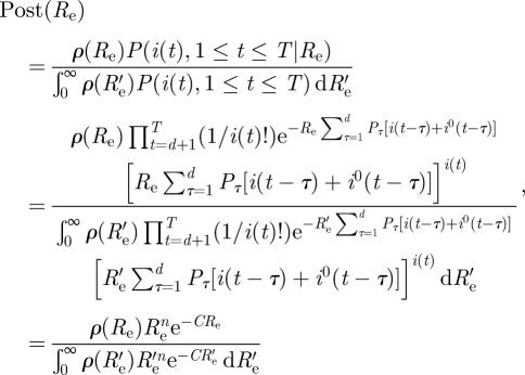where we have set , .

A standard Bayesian estimate for R_e is the mean of the posterior distribution, that is

Let us take the uniform (improper) prior ρ(R_e) ≡ 1, and evaluate .

Since , we obtain

Note that except for the insignificant difference of 1 in the numerator, is the same as the maximum likelihood estimate obtained before.

A useful measure of how precise the estimate is (that is how informative are the data), is to compute the variance σ² of the posterior distribution

Since

we obtain

Moreover, in the Bayesian approach, it is easy to find the 95% CI, that is an interval of R_e's on which 95 per cent of the probability is concentrated. Choosing this interval to be [ we just need to choose δ so that , that is , which is easy to do numerically.

We can also use the evaluation of σ² (in the case ρ (R_e) ≡ 1) given above to obtain an approximate 95% CI under the assumption that the posterior distribution is approximately normal. This is given by , so that an approximate credible interval for R_e is given by , where

References

- 1.Cohen J., Enserink M. 2009. Infectious diseases as swine flu circles globe, scientists grapple with basic questions. Science 324, 572–573 10.1126/science.324_572 (doi:10.1126/science.324_572) [DOI] [PubMed] [Google Scholar]
- 2.Miller M. A., Viboud C., Balinska M., Simonsen L. 2009. The signature features of influenza pandemics—implications for policy. New Engl. J. Med. 360, 2595–2598 10.1056/NEJMp0903906 (doi:10.1056/NEJMp0903906) [DOI] [PubMed] [Google Scholar]
- 3.Peiris J. S. M., Poon L. L. M., Guan Y. 2009. Emergence of a novel swine-origin influenza A virus (S-OIV) H1N1 virus in humans. J. Clin. Virol. 45, 169–173 10.1016/j.jcv.2009.06.006 (doi:10.1016/j.jcv.2009.06.006) [DOI] [PMC free article] [PubMed] [Google Scholar]
- 4.Lipsitch M., Riley S., Cauchemez S., Ghani A. C., Ferguson N. M. 2009. Managing and reducing uncertainty in an emerging influenza pandemic. New Engl. J. Med. 361, 112–115 10.1056/NEJMp0904380 (doi:10.1056/NEJMp0904380) [DOI] [PMC free article] [PubMed] [Google Scholar]
- 5.Roll U., Katriel G., Yaari R., Stone L., Barnea O., Mendelson E., Mendelboim M., Huppert A. Submitted Onset of a pandemic: characterizing the initial spread of swine flu (H1N1) epidemic in Israel. [DOI] [PMC free article] [PubMed] [Google Scholar]
- 6.WHO 2009. Changes in reporting requirements for pandemic (H1N1) 2009 virus infection. See http://www.who.int/csr/disease/swineflu/notes/h1n1_surveillance_20090710/en/. [Google Scholar]
- 7.Diekmann O., Heesterbeek J. A. P. 2000. Mathematical epidemiology of infectious diseases: model building, analysis and interpretation. Chichester, UK: Wiley [Google Scholar]
- 8.Keeling M. J., Rohani P. 2008. Modeling infectious diseases in humans and animals. Princeton, NJ: Princeton University Press [Google Scholar]
- 9.Kermack W. O., Mckendrick A. G. 1927. A Contribution to the mathematical theory of epidemics. Proc. R. Soc. Lond. A 115, 700–721 10.1098/rspa.1927.0118 (doi:10.1098/rspa.1927.0118) [DOI] [Google Scholar]
- 10.Murray J. D. 1989. Mathematical biology. Berlin, Germany: Springer [Google Scholar]
- 11.Carrat F., Vergu E., Ferguson N. M., Lemaitre M., Cauchemez S., Leach S., Valleron A. J. 2008. Time lines of infection and disease in human influenza: a review of volunteer challenge studies. Am. J. Epidemiol. 167, 775–785 10.1093/aje/kwm375 (doi:10.1093/aje/kwm375) [DOI] [PubMed] [Google Scholar]
- 12.Brauer F. 2008. Age-of-infection and the final size relation. Math. Biosci. Eng. 5, 681–690 10.3934/mbe.2008.5.681 (doi:10.3934/mbe.2008.5.681) [DOI] [PubMed] [Google Scholar]
- 13.Mccaw J. M., Mcvernon J., Mcbryde E. S., Mathews J. D. 2009. Influenza: accounting for prior immunity. Science 325, 1071–1071 10.1126/science.325_1071a (doi:10.1126/science.325_1071a) [DOI] [PubMed] [Google Scholar]
- 14.White L. F., Pagano M. 2008. A likelihood-based method for real-time estimation of the serial interval and reproductive number of an epidemic. Statist. Med. 27, 2999–3016 10.1002/sim.3136 (doi:10.1002/sim.3136) [DOI] [PMC free article] [PubMed] [Google Scholar]
- 15.White L. F., Wallinga J., Finelli L., Reed C., Riley S., Lipsitch M., Pagano M. 2009. Estimation of the reproductive number and the serial interval in early phase of the 2009 influenza A/H1N1 pandemic in the USA. Influenza Resp. Vir. 3, 267–276 10.1111/j.1750-2659.2009.00106.x (doi:10.1111/j.1750-2659.2009.00106.x) [DOI] [PMC free article] [PubMed] [Google Scholar]
- 16.Chowell G., Nishiura H. 2008. Quantifying the transmission potential of pandemic influenza. Phys. Life Rev. 5, 50–77 10.1016/j.plrev.2007.12.001 (doi:10.1016/j.plrev.2007.12.001) [DOI] [Google Scholar]
- 17.Chang C., et al. 2010. The novel H1N1 Influenza A global airline transmission and early warning without travel containments. Chinese Sci. Bull. 55, 3030–3036 10.1007/s11434-010-3180-x (doi:10.1007/s11434-010-3180-x) [DOI] [PMC free article] [PubMed] [Google Scholar]
- 18.Charland K. M. L., Buckeridge D. L., Sturtevant J. L., Melton F., Reis B. Y., Mandl K. D., Brownstein J. S. 2009. Effect of environmental factors on the spatio-temporal patterns of influenza spread. Epidemiol. Infect. 137, 1377–1387 10.1017/S0950268809002283 (doi:10.1017/S0950268809002283) [DOI] [PubMed] [Google Scholar]
- 19.Cruz-Pacheco G., Duran L., Esteva L., Minzoni A. A., Lopez-Cervantes M., Panayotaros P., Ahued Ortega A., Villaseñor Ruiz I. 2009. Modeling of the influenza A(H1N1)v outbreak in Mexico city, April–May 2009, with control sanitary measures. Eurosurveillance, 14, pii=19254 See http://www.eurosurveillance.org/ViewArticle.aspx?ArticleId=19254. [PubMed] [Google Scholar]
- 20.Fraser C., et al. 2009. Pandemic potential of a strain of influenza A (H1N1): early findings. Science 324, 1557–1561 10.1126/science.1176062 (doi:10.1126/science.1176062) [DOI] [PMC free article] [PubMed] [Google Scholar]
- 21.Hsieh H. 2010. Pandemic influenza A (H1N1) during winter influenza season in the southern hemisphere. Influenza and Other Respiratory Viruses 4, 187–197 10.1111/j.1750-2659.2010.00147.x (doi:10.1111/j.1750-2659.2010.00147.x) [DOI] [PMC free article] [PubMed] [Google Scholar]
- 22.Kelly H. A., Grant K. A., Williams S., Fielding J., Smith D. 2009. Epidemiological characteristics of pandemic influenza H1N1 2009 and seasonal influenza infection. Med. J. Austral. 191, 146–149 [DOI] [PubMed] [Google Scholar]
- 23.Mcbryde E. S., Bergeri I., van Gemert C., Rotty J., Headley E. J., Simpson K., Lester R. A., Hellard M., Fielding J. E. 2009. Early transmission characteristics of influenza A(H1N1)v in Australia: Victorian state 16 May–3 June 2009. Eurosurveillance 14, pii=19363 See http://www.eurosurveillance.org/ViewArticle.aspx?ArticleId=19363. [DOI] [PubMed] [Google Scholar]
- 24.Nishiura H., Castillo-Chavez C., Safan M., Chowell G. 2009. Transmission potential of the new influenza A(H1N1) virus and its age-specificity in Japan. Eurosurveillance 14, pii=19227 See http://www.eurosurveillance.org/ViewArticle.aspx?ArticleId=19227. [DOI] [PubMed] [Google Scholar]
- 25.Nishiura H., Wilson N., Baker M. G. 2009b. Estimating the reproduction number of the novel influenza A virus (H1N1) in a Southern Hemisphere setting: preliminary estimate in New Zealand. NZ Med. J. 122, 73–77 [PubMed] [Google Scholar]
- 26.Tuite A. R., et al. 2009. Estimated epidemiologic parameters and morbidity associated with pandemic H1N1 influenza. Can. Med. Assoc. J. 182, 131–136 10.1503/cmaj.091807 (doi:10.1503/cmaj.091807) [DOI] [PMC free article] [PubMed] [Google Scholar]
- 27.Hahne S., et al. 2009. Epidemiology and control of influenza A(H1N1)v in the Netherlands: the first 115 cases. Eurosurveillance 14, 2–5 [DOI] [PubMed] [Google Scholar]
- 28.Balcan D., et al. 2009. Seasonal transmission potential and activity peaks of the new influenza A(H1N1): a Monte Carlo likelihood analysis based on human mobility. BMC Med. 7 10.1186/1741-7015-7-115 (doi:10.1186/1741-7015-7-115) [DOI] [PMC free article] [PubMed] [Google Scholar]
- 29.ICDC 2010. Influenza activity weekly reports 2009–2010. See http://www.health.gov.il/english/pages_E/default.asp?maincat=15. [Google Scholar]
- 30.Greenbaum J., et al. 2009. Pre-existing immunity against swine-origin H1N1 influenza viruses in the general human population. Proc. Natl Acad. Sci. USA 106, 20 365–20 370 10.1073/pnas.0911580106 (doi:10.1073/pnas.0911580106) [DOI] [PMC free article] [PubMed] [Google Scholar]
- 31.Medlock J., Galvani A. P. 2009. Optimizing influenza vaccine distribution. Science 325, 1705–1708 10.1126/science.1175570 (doi:10.1126/science.1175570) [DOI] [PubMed] [Google Scholar]
- 32.Anderson R. M., May R. M. 1991. Infectious diseases of humans. New York, NY: Oxford university Press [Google Scholar]
- 33.Kanaan M. N., Farrington C. P. A. 2005. Matrix models for childhood infections: a Bayesian approach with applications to rubella and mumps. Epidemiol. Infect. 133, 1009–1021 10.1017/S0950268805004528 (doi:10.1017/S0950268805004528) [DOI] [PMC free article] [PubMed] [Google Scholar]
- 34.van Effelterre T., Shkedy Z., Aerts M., Molenberghs G., van Damme P., Beutels P. 2009. Contact patterns and their implied basic reproductive numbers: an illustration for varicella-zoster virus. Epidemiol. Infect. 137, 48–57 10.1017/S0950268808000563 (doi:10.1017/S0950268808000563) [DOI] [PubMed] [Google Scholar]
- 35.Wallinga J., Teunis P., Kretzschmar M. 2006. Using data on social contacts to estimate age-specific transmission parameters for respiratory-spread infectious agents. Am. J. Epidemiol. 164, 936–944 10.1093/aje/kwj317 (doi:10.1093/aje/kwj317) [DOI] [PubMed] [Google Scholar]
- 36.Wallinga J., Edmunds W. J., Kretzschmar M. 1999. Perspective: human contact patterns and the spread of airborne infectious diseases. Trends Microbiol. 7, 372–377 10.1016/S0966-842X(99)01546-2 (doi:10.1016/S0966-842X(99)01546-2) [DOI] [PubMed] [Google Scholar]
- 37.Mossong J., et al. 2008. Social contacts and mixing patterns relevant to the spread of infectious diseases. PLoS Med. 5, 381–391 10.1371/journal.pmed.0050074 (doi:10.1371/journal.pmed.0050074) [DOI] [PMC free article] [PubMed] [Google Scholar]
- 38.Fisman D. N., Savage R., Gubbay J., Achonu C., Akwar H., Farrell D. J., Crowcroft N. S., Jackson P. 2009. Older age and a reduced likelihood of 2009 H1N1 virus infection. New Engl. J. Med. 361, 2000–2001 10.1056/NEJMc0907256 (doi:10.1056/NEJMc0907256) [DOI] [PubMed] [Google Scholar]
- 39.Hancock K., et al. 2009. Cross-reactive antibody responses to the 2009 pandemic H1N1 influenza virus. New Engl. J. Med. 361, 1945–1952 10.1056/NEJMoa0906453 (doi:10.1056/NEJMoa0906453) [DOI] [PubMed] [Google Scholar]
- 40.Katriel G., Stone L. 2010. Pandemic dynamics and the breakdown of herd immunity. PLoS ONE 5, e9565. 10.1371/journal.pone.0009565 (doi:10.1371/journal.pone.0009565) [DOI] [PMC free article] [PubMed] [Google Scholar]