Abstract
We developed a maximum a posterior (MAP) reconstruction method for positron emission tomography (PET) image reconstruction incorporating magnetic resonance (MR) image information, with the joint entropy between the PET and MR image features serving as the regularization constraint. A non-parametric method was used to estimate the joint probability density of the PET and MR images. Using realistically simulated PET and MR human brain phantoms, the quantitative performance of the proposed algorithm was investigated. Incorporation of the anatomic information via this technique, after parameter optimization, was seen to dramatically improve the noise versus bias tradeoff in every region of interest, compared to the result from using conventional MAP reconstruction. In particular, hot lesions in the FDG PET image, which had no anatomical correspondence in the MR image, also had improved contrast versus noise tradeoff.
1. Introduction
PET imaging techniques provide important physiological and biochemical information for clinical diagnosis and scientific studies. However, even state-of-the-art PET imaging continues to be affected by limited spatial resolution and inherently noisy data (Rahmim and Zaidi 2008). Incorporation of anatomical information obtained from high-resolution MR or CT anatomical images may potentially improve the PET image quality and quantitative accuracy. The anatomical information is usually applied as priors in the Bayesian PET image reconstruction framework. There have been techniques using segmented anatomical images, in which regional boundaries or labels are produced, to penalize inter-voxel intensity variations within the regions (e.g. Lipinski et al 1997, Comtat et al 2002). More recent techniques (discussed next) tend to apply no segmentation of the anatomy but involve similarity measures that work directly on the image intensities. Improvements in reconstructed PET images for regions with corresponding anatomical boundaries have been widely reported. However, the effects of incorporating anatomy in detecting PET regions, particularly uptake lesions, that have no equivalent boundaries in the anatomical image, have not been as clearly studied and are still of much interest.
Bowsher et al (1996) presented a method that simultaneously segmented and reconstructed ECT (PET and SPECT) images. The assumption was made that radiopharmaceutical distribution could be modeled as consisting of regions, such that all voxels within a region had similar activities. A hierarchical image model was proposed with the number of regions and the regional classifications of individual voxels to be estimated as part of the reconstruction process. Voxel intensities in reconstructed ECT images were equated to the most probable regional mean activities given the anatomical segmentation as an initial estimate. When there were differences between ECT and anatomical segmentations, e.g. hot spots in brain stimulation studies or cold spots in arterial stenosis or occlusions, the anatomical penalty would cause underestimation of the lesion's volume in the reconstructed ECT images. To address this issue, the authors proposed to manually specify a loose region of interest (ROI) after the lesion was identified from the initial Bayesian reconstruction.
Rangarajan et al (2000) used the joint mixture framework to integrate the anatomical regional segmentation information into the Bayesian model. The prior was formulated to model the joint density between the anatomical and functional images. The mixture parametric density was specialized to a gamma distribution. The authors proposed a so-called EM2 algorithm with one EM step for reconstruction and the other EM step for parametric estimation of the joint mixture model. It was claimed that fewer hyperparameters (such as minimum region size, threshold for merging regions and others in Bowsher et al 1996) needed to be estimated, and furthermore, no user interaction was required. Conclusions were made that the approach introduced did not require the anatomical and functional regions to be exactly homologous. However, the designed lesion regions actually studied in this work did have corresponding boundaries in the anatomical image.
Somayajula et al (2005) proposed to use the mutual information between different features of MR/CT and PET images as priors in the reconstruction task. The applied features included the intensity, local mean in a neighborhood, and the horizontal and vertical gradients at each pixel. The method did not require anatomical segmentation information so it was not constrained by the accuracy of segmentation. A non-parametric method (in contrast with the parametric method used in Rangarajan et al 2000) was applied in the estimation of the joint density for mutual information calculation. The overall root-mean-square error in the reconstructed functional image with the mutual information prior was found to be much less than that with a quadratic prior. However, the anatomical and functional images used in the simulation study had identical boundary structure and were uniform within regions. The authors stated that the approach proposed was not expected to enhance lesions not visible in the anatomical image.
In an important contribution by Nuyts (2007), it was suggested that mutual information was not an optimal choice for the incorporation of anatomical side information in the MAP reconstruction as it caused bias in the reconstructed images. Instead, using only the joint entropy component of the mutual information as prior was proposed, and a gradient ascent algorithm was applied to update the emission image. For the emission image with an increased tracer uptake region that had no correspondence in the anatomical image, the performance of reconstruction algorithms with different priors was evaluated. Comparing the joint entropy prior with the conventional relative-difference prior, while some improvements were observed for regions with corresponding anatomy and function, no improvements were demonstrated in the functional region with no anatomical counterpart.
In this paper, we have designed and investigated a one-step-late (OSL) maximum a posteriori (MAP) algorithm incorporating the joint entropy between features of the anato-functional image pairs as the prior. Using simulated brain imaging studies, we optimized the parameters characterizing the reconstruction algorithm. The performance of this proposed technique was then evaluated, especially in terms of recovering functional regional lesion with no corresponding region (or structural boundary) in anatomy. The quality of images reconstructed from the proposed algorithm was in particular compared with that of images from conventional `smoothness' prior to MAP reconstruction.
2. Methods
2.1. Proposed MAP reconstruction method
The proposed technique incorporates non-parametrically estimated joint entropy prior (between MR and PET) within the MAP PET image reconstruction algorithm. We will describe the general MAP reconstruction formulation, followed by the joint entropy prior specifications. The MAP estimate of a functional image f from the emission sinogram data g is given by
| (1) |
The expression P() indicates the probability of the variable enclosed in parentheses. Assume that the prior P(f) follows a Gibbs distribution of the form
| (2) |
where W is a normalization factor, β is a positive constant and V(f) is the potential function, which has conventionally been utilized to penalize inter-voxel intensity variations.
Seeking the solution of f to (1) is equivalent to finding that maximizes the log-posterior probability:
| (3) |
where the constant k represents the contribution of the W term in (2) and the denominator in (1). Applying the Poisson statistics to the first term of (3), the iterative procedure is derived as what was done by Green (1990):
| (4) |
where the new estimate of voxel i in the image vector f is updated from the old estimate. A single bin j of the measured emission data g is represented by gj, and cij represents an element of the projection matrix C, modeling the contribution of voxel i to projection bin j. Note that the OSL strategy involves calculation of the derivative of V(f).
The method proposed in this work sets the V(f) term in the prior (2) as the joint entropy of random vectors extracted from the functional and the anatomical images. Assume that the N feature vectors extracted from the functional and anatomical images are represented by xi and yi, respectively for i = 1, 2, …, N. These feature vectors can be considered as realizations of random feature vectors X and Y. Note that when we use only one feature, e.g. the intensity of the two images (which is the case in this work), then x and y represent the functional and anatomical images, respectively. These feature vectors, x and y, are then considered as realizations of the random feature variables X and Y.
The joint entropy of the two random feature vectors HX,Y can be evaluated by constructing the vector random variable Z = [X, Y]T. The entropy of the random variable HZ may be expressed as
| (5) |
where the summation is performed over all possible values of the vector random variable Z. The probability density p(Z) is approximated by a superposition of Gaussian densities centered on the realizations zj of a sample S drawn from Z (Duda et al 2001):
| (6) |
where NS is the number of realizations of Z in the sample S,
| (7) |
and n is the dimension of Z. The use of the Gaussian density (7) in the Parzen density estimate (6) simplifies the subsequent analysis but is not necessary (Viola 1995).
The estimation of HZ depends on the covariance ψZ of the multi-dimensional Parzen window functions that are used in the probability density estimation of Z. Assume that this covariance matrix is diagonal ψZ = DIAG(ψXX, ψYY), ψXX and ψYY being the diagonal covariance matrices for the functional and anatomical image feature vectors, respectively. Since the present work considers the image intensity as the only feature of interest, the joint probability density p(X, Y) can then be estimated by
| (8) |
With the joint entropy of intensity extracted from the functional and anatomical images serving as the potential function, the derivative of in (4) becomes . Unlike other works in which the covariance matrix ψXX of a PET image was assumed to have uniform of diagonal entries, we choose the following model:
| (9) |
in which each element of the covariance matrix is assumed proportional to squared voxel intensity. This was motivated by previous investigations into the EM algorithm (Barrett et al 1994).1 The derivative of the joint entropy is then
| (10) |
where the summation is performed over all possible values of X and Y.
2.2. Conventional MAP reconstruction method
For comparison purposes, we have also implemented a conventional MAP algorithm using a `smoothness' prior, as selected by Green (1990):
| (11) |
where δ is a parameter and wi,j is a weight indicating the strength of neighborliness between pixels i and j. The weight wi,j is set to 1 if i and j are orthogonal nearest neighbors, to for diagonal neighbors and to 0 otherwise. The function φ, which is supposed to be nonnegative and symmetric about 0 and monotonically increasing for positive values of its arguments, is set to
| (12) |
We note that the derivative of this term is
| (13) |
Therefore, the derivative insertion in (4) as of V (f) with respect to fi is calculated as (based on the assumption of independent fi and fj)
| (14) |
2.3. Phantom simulation
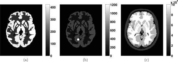
We used a newly developed mathematical human brain phantom (Rahmim et al 2008) for the purpose of performing realistic simulations.2 The brain phantom was constructed using subdivision surfaces (Hoppe et al 1994), which can be used to efficiently model structures with an arbitrary topological type, such as the brain, skull, muscle tissue and vasculature. Surfaces were modeled based on a segmented MRI dataset of a normal subject, with 100 structures identified and modeled. The PET activities in the various regions of the brain were specified based on a clinical FDG study (figure 1(a)). Additionally, a corresponding MRI image was generated based on actual patient MR intensity measurement (figure 1(c)).
Figure 1.
Transaxial slice of the human brain phantoms simulating activities of (a) PET, (b) PET with a designed lesion and (c) MRI.
To test the MAP algorithms described above, we performed analytical simulations of the functional brain phantom with a designed hot lesion globe on the medial occipitotemporal gyrus region (figure 1(b)). Lesions of different sizes (with the radii of 4.2 mm, 5.8 mm and 8.2 mm) were tested and the one shown in figure 1(b) has a radius of 4.2 mm, with a hot/background ratio of 3:1. The lesions were incorporated to evaluate whether the proposed technique outperforms the conventional technique in this scenario. To achieve reconstructed images of 128 × 128 × 47 voxels with each voxel size as 2.34 × 2.34 × 3.27 mm3, we used a finer grid brain phantom with a reduced voxel size by a factor of 2 in each dimension. Data were simulated for the geometry of the Discovery RX PET/CT scanner (Kemp et al 2006), except with the transaxial dimensions (crystal dimensions and field of view) scaled by 0.5 to simulate a dedicated brain scanner. After projection, 31 noise realizations were implemented with the Poisson noise level consistent with routine clinical FDG brain PET count rate levels. Attenuation and normalization effects were incorporated within the simulations; these effects were also incorporated within the reconstruction.
2.4. Evaluation metrics
To quantitatively evaluate the reconstructed image quality, we used the tradeoff between the normalized mean squared error (NMSE), as a measure of bias, and the normalized standard deviation (NSD), as a measure of noise, for individual areas of the brain. To calculate the NMSE, the finer grid phantom used for data generation was collapsed to the size of the reconstructed image to serve as the reference true image. The NMSE for each ROI covering one area of the brain was calculated using
| (15) |
where and ; denotes the ith reconstructed voxel intensity from the jth noise realization and μi denotes the reference true activity value; n is the number of voxels in the ROI and m is the number of noise realizations. We adopted such an ROI-based definition as we believe it should minimize the effect of voxel noise on this bias-measuring metric. For each ROI, the NMSE bias value was plotted against the NSD noise value, as calculated using
| (16) |
where , n and m were defined as those in (15); representing the ensemble mean value of voxel i.
To quantify the ability of a given reconstructed image to recover the contrast between the lesion and normal background areas, we calculated the contrast recovery ratio. The average contrast from the m noise realizations was defined by
| (17) |
where and are the average value from the normal (N) and defect (D) regions of the jth noise realization, respectively. The contrast recovery ratio was calculated as the ratio between the contrast estimated from the reconstructed image and the true contrast in the phantom image.
3. Results
We evaluated the proposed and conventional MAP algorithms in the reconstruction of simulated noisy projection data of the brain phantom with a lesion. The parameters in the two algorithms were first optimized separately using one noise realization of the projection data, followed by comparison in terms of regional noise versus bias performance over the other 30 noise realizations. Furthermore, we specifically evaluated the algorithms in terms of the lesion contrast recovery versus noise property. The performance of the reconstruction algorithm was found to be similar with different lesion sizes when evaluated using the metrics described above; therefore, we only present the results from the lesion size shown in figure 1.
3.1. Parameter optimization
The performance of a MAP reconstruction algorithm strongly depends on the construction of the prior and the weighting factor (β in (4)), which determines how much a role the prior plays in the reconstruction process. Before comparing the proposed MAP algorithm with the conventional MAP algorithm, we first optimized their performance using one noise realization of the projection data based on the tradeoff between the NSD and the NMSE.
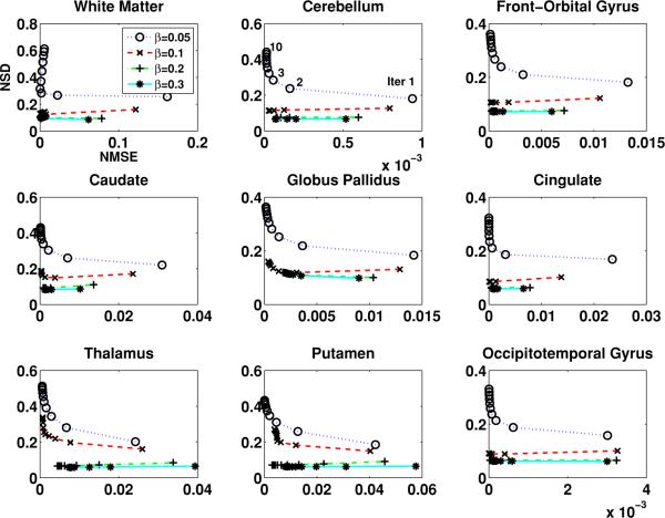
For the proposed MAP algorithm, we studied the effect of the scaling factor α in (9) with fixed β-values. This factor α determines the Gaussian density covariance in the Parzen windows added to estimate the joint probability density in (8). Through extensive testing, we found the range of α from 0.2 to 0.07 resulted in considerably better regional NSD versus NMSE tradeoffs compared to the results of the maximum likelihood EM (MLEM) algorithm. Within the above-mentioned range, smaller α-values generated slightly better results while reducing α further did not lead to reasonable reconstructed images. This may imply that a Parzen window variance that is too small would not produce a proper estimate of the image probability density. With the optimized α, the effect of β (within the reasonable range selected) on the noise versus bias tradeoff in representative individual brain regions is shown in figure 2. Each curve in the plots presents the NSD versus NMSE variation with the increased iteration number (with one iteration containing 21 subsets). The performance of the proposed MAP algorithm with one β is easily compared with another. For the same NMSE, if one curve corresponds to a lower NSD than another, this would indicate superior quantitative performance in terms of noise versus bias tradeoff. Among the β-values plotted, the improvement in image quality was achieved when β was increased from 0.05 to 0.2. Increasing β to 0.3 did not further reduce the NSD while sacrificing the NMSE. We thus utilized β = 0.2 as the choice for the proposed joint-entropy-incorporated MAP method to compare its performance with the conventional method, which we also optimized (δ in (14) and β) accordingly. As a side note, increasing the value of β more from the above-mentioned values generated negative image updates in some instances. This issue could be addressed in practice by imposing an image non-negativity constraint, in which such negative updates would not be applied in the particular iteration (subset) as they appeared (Rahmim et al 2004, 2005). However, to emphasize, upon the use of β values close to the optimized one, such negative updates were not encountered.
Figure 2.
The NSD versus NMSE for different regions of the brain image (from one noise realization of projection data) changing with the iteration number, using different β in the joint-entropy-incorporated MAP algorithm.
3.2. Performance comparison
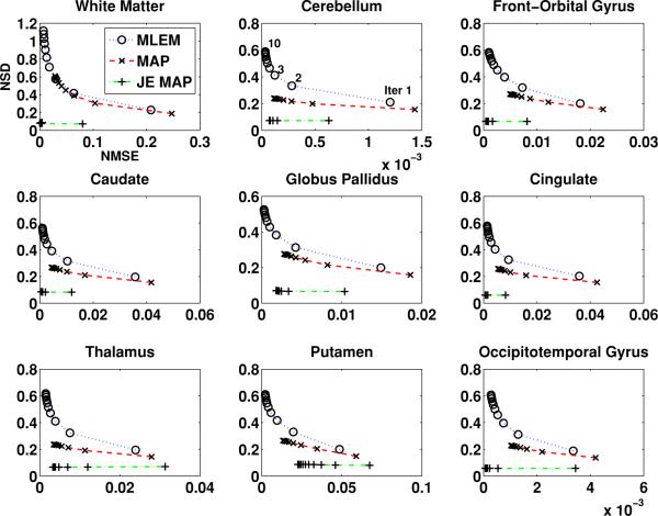
Following the optimization of parameters (also see section 4), we compared the performance of reconstruction algorithms, over 30 noise realizations other than the noise realization optimization were performed on. The comparison was also in terms of the regional image quality defined by the noise versus bias tradeoff. Figure 3 shows the regional NSD versus NMSE variation along with iteration number plots of images reconstructed using the proposed joint-entropy-incorporated MAP algorithm and the conventional MAP algorithm. The results from using the MLEM algorithm without any prior information are also displayed. As depicted in plots for the individual ROIs, applying prior information through both the joint-entropy-based method and the conventional method improved the noise versus bias tradeoff of reconstructed image. The improvement is seen to be more significant from the proposed MAP method compared to that from the conventional MAP method. It is also worth noting that with the proposed joint-entropy-based method, the image noise level stabilizes even as the iteration number increases.
Figure 3.
The NSD versus NMSE changing with the iteration number (from 30 noise realizations of projection data) for different regions of brain images reconstructed, from (i) the MLEM algorithm (MLEM), (ii) the conventional MAP algorithm (MAP) and (iii) the joint-entropy-incorporated MAP algorithm (JE MAP).
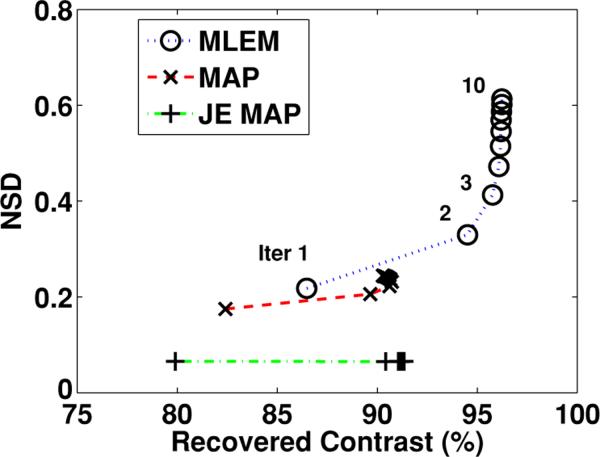
One of the major motivations for the incorporation of anatomical information within the emission image reconstruction process is to improve the performance in detecting and quantifying functional regions with no anatomical correspondence (e.g. increased uptake at brain stimulation study). We specifically evaluated the image reconstruction algorithms in terms of recovering the designed hot lesion. Figure 4 shows variation of the NSD versus lesion contrast recovery ratio. As demonstrated, a better noise versus contrast recovery ratio was achieved by the proposed joint-entropy-incorporated MAP algorithm, compared to the conventional MAP algorithm (with comparable contrast, noise was further reduced).
Figure 4.
The NSE versus contrast recovery ratio changing with the iteration number for the region with the lesion, from (i) the MLEM algorithm, (ii) the conventional MAP algorithm and (d) the joint-entropy-incorporated MAP algorithm.
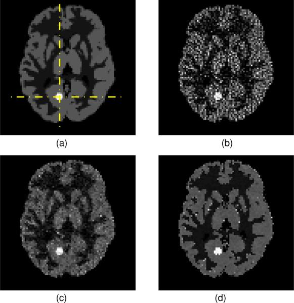
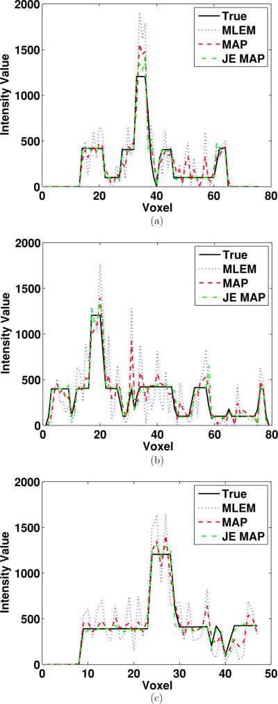
In order to gain a more direct impression of the reconstructed images from different algorithms, we show the transaxial image slices containing the centroid of the lesion. The phantom image (with grid one-half coarser than the one shown in figure 1) and the reconstructed images from using the MLEM algorithm and the two MAP algorithms are presented in figure 5. The improvement in image quality reconstructed from the joint-entropy-incorporated MAP algorithm is rather obvious. The profiles of transaxial horizontal and vertical lines crossing the centroid of the lesion are shown in figures 6(a) and (b), respectively. The profile of the axial line perpendicular to the shown slice, passing through the cross point of the horizontal and vertical lines, is shown in figure 6(c). From these profiles, we see that the conventional MAP algorithm reduces noise at the same time reducing the contrast (less sharp region edges), when compared to the MLEM algorithm. It is also clearly demonstrated that the joint-entropy-incorporated MAP method lowers the noise in different regions while keeping the edges between regions sharp.
Figure 5.
Transaxial slice containing the lesion centroid of (a) the phantom image, (b) the image reconstructed from the MLEM algorithm, (c) the image reconstructed from the conventional MAP algorithm and (d) the image reconstructed from the joint-entropy-incorporated MAP algorithm.
Figure 6.
(a) Horizontal, (b) vertical and (c) perpendicular axial line profiles crossing the centroid of the lesion.
4. Discussion
A key behind the marked qualitative and quantitative improvements observed using the proposed technique has been to systematically optimize the designated parameters. The effect of selection of parameters including β in (4) and α in (9) has been discussed in the last section. As mentioned, the probability density estimation depends on the Parzen window sizes determined by α, while its incorporation within the algorithm is controlled by the weighting factor β. In addition, the probability estimation involves two other factors besides the window sizes, which are the intensity (color) sampling (Z in (6), therefore X, Y in (10)) and the spatial sampling (S in (6)) as we describe next.
The intensity sampling of X, Y in (10) involves the choice of the number of bins and the upper intensity (while the lower intensity is set to 0). The number of bins needs to be sufficient to distinguish regions with close intensities. The upper intensity value needs to be changed along with iterations since the maximum value of the updated image tends to continuously increase. It was found that the upper intensity value had to be set larger than the current maximum value for properly sampling the probability density. This was because the probability density estimation involved Gaussian densities centered on the sampled intensities (including range of intensities around and thus slightly above the maximum sampled intensity). This proper sampling was proved necessary to suppress the growth of the maximum value voxels along with iterations.
Calculation of the derivative of the joint entropy, especially when the probability density (8) is estimated by sampling every voxel in the images, can be quite computationally demanding. An alternative approach has been to sample only every few voxels, thus reducing the computation of the first term () in (10). The derivative term in (10), which is less computation-intensive, is still performed at each voxel as required by the iterative MAP algorithm. We studied the effect of spatial sampling rates on estimating probability density in Tang et al (2008). It was found that using one voxel every four voxels in the simulated FDG image still reached estimation of the probability density very close to that acquired from using every voxel in the entire image. Interestingly, the spatial sampling makes the simplification assumption of diagonal covariance matrix more justified since the sampled voxels are spatially more separated and less correlated.
In the study presented here, we have used mathematical quality evaluation criteria to optimize the aforementioned parameters. In the future, we wish to perform task-based parameter optimization using the computer observer study, as well as overall statistical receiver operating characteristic (ROC) analysis to compare the proposed technique with conventional MLEM and MAP image reconstruction approaches.
5. Summary
We developed an OSL MAP reconstruction algorithm for brain PET image reconstruction using the joint entropy of anatomical and functional image features as the regularization constraint. Non-parametric Parzen estimation of the probability density was performed, wherein the elements of the diagonal covariance matrix of the PET image were assumed to be proportional to squared individual voxel intensities, instead of being identical for different intensities. Using simulation studies with PET and MR brain phantoms, we optimized the performance of this proposed algorithm and compared its performance with a conventional MAP algorithm and the MLEM algorithm. The effect of the prior weighting factor on the quality of PET images reconstructed from the joint-entropy-incorporated MAP algorithm was studied quantitatively, using the regional NSD versus NMSE tradeoff as measures of image noise and bias. The optimized joint-entropy-incorporated MAP algorithm improved the image quality more dramatically than the conventional MAP algorithm, compared to the MLEM algorithm. Furthermore, for functional lesions with no corresponding anatomic counterpart, at any given reconstructed lesion contrast recovery, the proposed MAP algorithm achieved the lower noise level than the other two algorithms examined.
Acknowledgments
This work was supported by the Siemens Medical Solutions grant JHU-MR-33-01. The authors wish to thank Dr Hiroto Kuwabara for consultation on realistic brain MRI and PET simulations and Mr Andy Crabb for assistance with computational facilities.
Footnotes
Furthermore, inspection of the variance image generated from reconstructed images of multiple noise realizations simulated in this work, and quantitative comparison with squared intensities of the reconstructed image from a single noise realization, was seen to provide more justification for this model.
The human brain phantom is shared for public use at http://www.jhu.edu/rahmim/brain_phantom.html.
References
- Barrett HH, Wilson DW, Tsui BMW. Noise properties of the EM algorithm: I. Theory. Phys. Med. Biol. 1994;39:833–46. doi: 10.1088/0031-9155/39/5/004. [DOI] [PubMed] [Google Scholar]
- Bowsher JE, Johnson VE, Turkington TG, Jaszczak RJ, Floyd CE, Jr, Coleman RE. Bayesian reconstruction and use of anatomical a priori information for emission tomography. IEEE Trans. Med. Imaging. 1996;15:673–86. doi: 10.1109/42.538945. [DOI] [PubMed] [Google Scholar]
- Comtat C, Kinahan PE, Fessler JA, Beyer T, Townsend DW, Defrise M, Michel C. Clinically feasible reconstruction of 3D whole-body PET/CT data using blurred anatomical labels. Phys. Med. Biol. 2002;47:1–20. doi: 10.1088/0031-9155/47/1/301. [DOI] [PubMed] [Google Scholar]
- Duda RO, Hart PE, Stork DG. Pattern Classification. 2nd edn Wiley; New York: 2001. [Google Scholar]
- Green PJ. Bayesian reconstructions from emission tomography data using a modified EM algorithm. IEEE Trans. Med. Imaging. 1990;9:84–93. doi: 10.1109/42.52985. [DOI] [PubMed] [Google Scholar]
- Hoppe H, DeRose T, Duchamp T, Halstead M, Jin H, McDonald J, Schweitzer J, Stuetzle W. Piecewise smooth surface reconstruction. Comput. Graph. 1994;28:295–302. [Google Scholar]
- Kemp BJ, Kim C, Williams JJ, Ganin A, Lowe VJ. NEMA NU 2-2001 performance measurements of an LYSO-based PET/CT system in 2D and 3D acquisition modes. J. Nucl. Med. 2006;47:1960–7. [PubMed] [Google Scholar]
- Lipinski B, Herzog H, Rota Kops E, Oberschelp W, Muller-Gartner HW. Expectation maximization reconstruction of positron emission tomography images using anatomical magnetic resonance information. IEEE Trans. Med. Imaging. 1997;16:129–36. doi: 10.1109/42.563658. [DOI] [PubMed] [Google Scholar]
- Nuyts J. The use of mutual information and joint entropy for anatomical priors in emission tomography. IEEE Nucl. Sci. Symp. Med. Imaging Conf. Rec. 2007;6:4149–54. [Google Scholar]
- Rahmim A, Cheng JC, Blinder S, Camborde M-L, Sossi V. Statistical dynamic image reconstruction in state-of-the-art high resolution PET. Phys. Med. Biol. 2005;50:4887–912. doi: 10.1088/0031-9155/50/20/010. [DOI] [PubMed] [Google Scholar]
- Rahmim A, et al. Accurate event-driven motion compensation in high-resolution PET incorporating scattered and random events. IEEE Trans. Med. Imaging. 2008;27:1018–33. doi: 10.1109/TMI.2008.917248. [DOI] [PMC free article] [PubMed] [Google Scholar]
- Rahmim A, Lenox M, Reader AJ, Michel C, Burbar Z, Ruth TJ, Sossi V. Statistical list-mode image reconstruction for the high resolution research tomograph. Phys. Med. Biol. 2004;49:4239–58. doi: 10.1088/0031-9155/49/18/004. [DOI] [PubMed] [Google Scholar]
- Rahmim A, Zaidi H. PET versus SPECT: strengths, limitations and challenges. Nucl. Med. Comm. 2008;29:193–207. doi: 10.1097/MNM.0b013e3282f3a515. [DOI] [PubMed] [Google Scholar]
- Rangarajan A, Hsiao I-T, Gindi G. A Bayesian joint mixture framework for the integration of anatomical information in functional image reconstruction. J. Math. Imaging Vis. 2000;12:199–217. [Google Scholar]
- Somayajula S, Asma E, Leahy RM. PET image reconstruction using anatomical information through mutual information based priors. IEEE Nucl. Sci. Symp. Conf. Rec. 2005;5:2722–6. [Google Scholar]
- Tang J, Tsui BMW, Rahmim A. Bayesian PET image reconstruction incorporating anato-functional joint-entropy. IEEE Int. Symp. on Biomedical Imaging. 2008:1043–6. doi: 10.1088/0031-9155/54/23/002. [DOI] [PMC free article] [PubMed] [Google Scholar]
- Viola PA. Alignment by maximization of mutual information PhD Thesis Massachusetts Institute of Technology. 1995. [Google Scholar]


