Detecting common copy number variants in high-throughput sequencing data by using JointSLM algorithm

Abstract

The discovery of genomic structural variants (SVs), such as copy number variants (CNVs), is essential to understand genetic variation of human populations and complex diseases. Over recent years, the advent of new high-throughput sequencing (HTS) platforms has opened many opportunities for SVs discovery, and a very promising approach consists in measuring the depth of coverage (DOC) of reads aligned to the human reference genome. At present, few computational methods have been developed for the analysis of DOC data and all of these methods allow to analyse only one sample at time. For these reasons, we developed a novel algorithm (JointSLM) that allows to detect common CNVs among individuals by analysing DOC data from multiple samples simultaneously. We test JointSLM performance on synthetic and real data and we show its unprecedented resolution that enables the detection of recurrent CNV regions as small as 500 bp in size. When we apply JointSLM to analyse chromosome one of eight genomes with different ancestry, we identify 3000 regions with recurrent CNVs of different frequency and size: hierarchical clustering on these regions segregates the eight individuals in two groups that reflect their ancestry, demonstrating the potential utility of JointSLM for population genetics studies.

INTRODUCTION

The discovery of structural variants (SVs), including copy number variants (CNVs) and balanced rearrangements such as inversions and translocations, is deeply changing our understanding of the human genotype (2,1). Recently, multiple studies have discovered an abundance of structural variations of DNA segments that range from kilobases (kb) to megabases (Mb) in size (3). SVs have been found among normal individuals (4–6) while others participate in causing various disease states (7). For instance, genetic variants associated with cancer often result from rearrangements and alterations in proto-oncogenes or tumour suppressor genes (8–10), and Alzheimer and Parkinson's diseases have been associated with changes in gene dosage resulting from alterations in copy number (11,12).

In the last decade SVs detection has been performed with microarray technologies. The high-density CGH arrays (aCGH) and SNP genotyping arrays afford a level of resolution that allows CNV boundaries to be called with relatively high precision at a genome-wide level. However, although microarray platforms have been successfully used to identify CNVs, their resolution is limited by either the density of the array itself (for aCGH) or by the density of known SNP loci (for SNP arrays). For instance, currently available array platforms that consist of more than 1 million probes have a lower limit of detection of ∼5 to 10 kb (6,13).

Over recent years, the advent of new high-throughput sequencing (HTS) platforms, such as Illumina's Genome Analyzer and ABI's SOLiD, have opened many opportunities for SV discovery and has enabled initiatives such as the 1000 Genomes project (http://www.1000genomes.org) that aims to sequence the genomes of more than 1000 individuals to extend our knowledge on human genetic variation. HTS technologies are able to sequence a full human genome per week generating milions of short nucleotide sequences in a single instrument run.

The first HTS-based approach to detect SVs were based on paired-end read mapping (PEM), which identifies insertions and deletions by comparing the distance between mapped read pairs to the average insert size of the genomic library. Although this method is able to identify deletions smaller than 1 kb with high sensitivity, it does not allow the discovery of insertions larger than average insert size of the library and the exact borders of SVs in complex genomic regions rich in segmental duplication (14,15).

In this scenario, a very promising approach for the identification of SVs using HTS technologies consists in measuring the depth of coverage (DOC) of reads aligned to the human reference genome (15). At present, few computational methods have been developed for the analysis of DOC data: Campbell et al. (16) use the Circular Binary Segmentation algorithm (17) originally developed for genomic hybridization microarray data, Chiang et al. (18) use a local change-point analysis technique, while Yoon et al. (19) developed a new method based on the significance testing that works on intervals of data points. Although these algorithms are very sensitive and specific in discovering SVs from DOC data, they allow to analyse only one sample at time. The simultaneous analysis of multiple samples can improve statistical strength in the identification of signals shared by the data, increasing the resolution of SVs detection. Moreover, the identification of signals shared by multiple samples can lead to the detection of regions of interest since disease-critical genes are more likely to be found in regions that are common or recurrent among samples.

For these reasons, we have developed a novel algorithm, named JointSLM, that allows to analyse DOC signals from multiple samples simultaneously for the identification of common DNA events (recurrent CNVs) across individuals. By means of simulated data, we show that our algorithm is able to sensitively and accurately detect common structural variants as small as 500 bp in size. The comparison with other three state of the art methods show that our joint model allows one to obtain an unprecedented resolution in the detection of recurrent CNVs. We applied JointSLM to the DOC data of eight genomes and we demonstrate its unique advantage in population-based studies.

MATERIALS AND METHODS

DOC

HTS technologies, such as Illumina's Genome Analyzer and ABI's SOLiD, are able to generate milions of short nucleotide sequences in a single instrument run. Assuming the sequencing process is uniform, the number of reads mapping to a region follows a Poisson distribution and is expected to be proportional to the number of times the region appears in the DNA sample: a genomic region that has been deleted (duplicated) will have less (more) reads mapping to it than a region not deleted (duplicated).

Following this assumption, the copy number of any genomic region can be estimated by counting the number of aligned reads to the reference genome. Campbell et al. (16) and Chiang et al. (18) were the firsts to use this approach to detect copy-number alterations between tumour and healthy samples of the same individuals, while more recently Yoon et al. (19) proposed to use the read count in sequence data to look for genomic regions that differ in copy number between normal individuals of the 1000 genomes project.

The strategy to obtain DOC data consists in counting the number of mapped reads in non-overlapping windows of fixed length and then correcting each window by GC content: Campbell et al. (16) and Chiang et al. (18) used the logarithm of the ratio between the number of aligned reads from a tumour sample and the match normal sample, while Yoon et al. (19) used the number of aligned reads every 100-bp, corrected for GC content and median normalized to copy number 2 [median normalization is defined as 2 × (read count)/(mean read count over the genome) for each sample]. The DOC data obtained with this approach is mathematically very similar to the signal obtained from aCGH log₂ ratios. Deletions or duplications are identified as a decrease or increase in coverage across multiple consecutive windows. Moreover, like aCGH log₂-ratios, DOC sequences have noise caused by mapping errors and random fluctuations in genome coverage. For these reasons, the events in DOC can be detected using the same types of segmentation algorithms that are used for aCGH data.

In a recent paper (20), we developed a fast and powerful algorithm to segment aCGH data in which the log₂ ratios were modelled as a sum of two independent stochastic processes by means of Shifting Level Model (SLM). Due to their similarity with aCGH genomic profiles, also DOC genomic profiles can be considered to be generated by the sum of two processes: a biological process due to a real variation of the number of DNA copies and a white noise process that mimics experimental error.

Here, we introduce a novel method that extend the SLM algorithm from the classical univariate form to a multivariate form to segment multiple DOC signals simultaneously for the identification of common alterations. For each sample studied in this work, we take into consideration the logarithm in base 2 of the median-normalized DOC data obtained as in Yoon et al. (19): DOC was measured by counting the number of mapped reads in 100-bp windows, correcting for GC content and then median-normalizing to copy number 2. The 100-bp windows were chosen because at 30x coverage, the distribution of read counts is well approximated by a normal distribution, thus permitting us to assume normality in our mathematical modelling. DOC data from multiple samples were modelled as a sequential processes made of N observation each.

The multivariate form of the SLM

We consider M sequential processes (samples) with N observations each (100-bp windows) and we denote with t (t = 1, … , M) and i (i = 1, … , N) the respective indexes. We model the sequential process x = x₁, … , x_i, … , x_N, where x_i = (x_i1, … , x_iM)′, as the sum of two independent stochastic processes:

(1)

(2)

where m_i = (m_i1, … , m_iM) is the vector of the unobserved mean level and ϵ_i is the vector of white noises. The white noise vector ϵ_i follows a multivariate normal distribution with mean μ_ϵ = [0] and covariance matrix Σ_ϵ; z_i are random variables taking the values in [0, 1] with probabilities η = Pr(z_i = 1), 1 − η = Pr(z_i = 0); δ_i are random vectors that follow a multivariate normal distribution and μ_i is the vector of the means.

The process m_i is controlled by the process z_i : when z_i−1 = 0, m_i is the same as m_i−1 and when z_i−1 = 1, m_i takes its new value according to a multivariate Gaussian law with mean μ and covariance matrix Σ_ϵ independently of m_i−1:

(3)

(4)

Combining the definitions given above, the joint distribution of the observations and latent variables, given the parameters, has the following form:

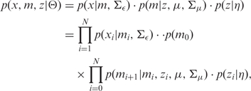(5)

where Θ = (μ, Σ_μ, Σ_ϵ, η).

Since the DOC data are modelled as the sum of two independent stochastic processes, the expected value of x_i is equal to μ and its covariance matrix is given by the sum of the covariances of the two processes:

(6)

(7)

Using (7) we can introduce a different parametrization of the SLM by defining the parameter ω such that Σ_μ = ω · Σ and Σ_ϵ = (1–ω) · Σ.

When we deal with multiple DOC signals (profiles) simultaneously, we have to take into account some fundamental considerations: (i) each DOC profile is characterized by its technical noise caused by mapping errors and random fluctuations in genome coverage and (ii) in each DOC profile, a CNV can be present at variable copy number in comparison with a reference genome. For these reasons, the white noise distributions and mean level distributions can be considered independent across samples and we can write:

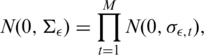(8)

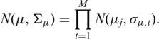(9)

where σ_ϵ,t and σ_μ,t are the standard deviations of the normal distribution of the t-th sequential process for the white noise and the mean level distributions, respectively.

With these assumptions, from a mathematical point of view, the random process z_i is the only variable that correlates the samples. When z_i changes its value, the mean level of each sample have a shift. In this way, our joint model is able to detect common shift in the mean of multiple samples.

The JointSLM algorithm

The joint distribution of Equation (5) defines an Hidden Markov Model (HMM) of order one with state variable q_i = (m_i, z_i) and multivariate emission probability (see Supplementary Data). The fact that the multivariate SLM is an HMM allows us to make use of the several algorithms developed for these kinds of models.

To estimate the parameters of the Multivariate SLM, we develop a two step algorithm that follows the idea of (20), based on dynamic programming. The inputs to the algorithm are the sequences x = {x₁, … , x_M} to be jointly segmented, the initial estimate of the number of states K₀ and the parameters ω and η. In the first step, we estimate the parameters m_i by means of the Baum and Welch re-estimation strategy (21), while in the second step we estimate the best state sequence s (the z_i variables, i.e. the points of mean shift) by means of the Viterbi algorithm. Finally, we convert the data from log space to copy number space and we calculate the median of the data that belong to each segment. A detailed description of the algorithm and the study of the effect of the parameters K₀, ω and η on the performance of JointSLM are reported in Supplementary Data.

RESULTS

Synthetic data analysis

To assess the performance of JointSLM algorithm in identifying common DNA events of different size, we made an intensive simulation based on synthetic data generated from the GC-adjusted DOC data of chromosomes 1 and X of the male individual NA18507. To estimate specificity, we generated synthetic chromosomes by sampling 10 000 100-bp windows from chromosome 1 to simulate normal copy number. To estimate sensitivity, we added to the normal copy number chromosomes nine deletions of size 200 bp, 300 bp, 400 bp, 500 bp, 700 bp, 1 kb, 2.5 kb, 5 kb and 10 kb sampled from chromosome X. To minimize the sampling of random false positives we removed all gaps, segmental duplications, telomeres/centromeres and regions with known CNVs from the Database of Genomic Variants (DGV, http://projects.tcag.ca/variation/) and the Genome Structural Variation Consortium (GSV, http://www.sanger.ac.uk/humgen/cnv/42mio/).

We applied JointSLM with different parameter settings on data sets made of 10, 30 and 50 normal copy number chromosomes, and we evaluated false positive rate (FPR) by counting the number of detected alterations. The specificity of the algorithm can be controlled by the parameters η and ω (see Supplementary Data): the higher are the values of η and ω and the larger is the number of detected false positive (FP) events. For instance, in the 10 samples analysis (Figure 1b), when we set η = 10⁻³ and ω = 0.3 we detect an average of 9.4 FP events that range between 100 and 500 bp in size (6.0 events of 100 bp, 2.6 of 200 bp, 0.62 of 300 bp, 0.12 of 400 bp and 0.08 of 500 bp), while using a more conservative set of parameters (η = 10⁻⁶ and ω = 0.1), we detect an average of 0.91 FP events (0.66 of 100 bp, 0.22 of 200 bp, 0.02 of 300 bp and 0.01 of 400 bp). In the analysis of the 30 samples data set (Supplementary Figure), we detected an average of 21.6 FP events (FPR = 0.2%) with ω = 0.3 and η = 10⁻³ and an average of 9.6 (0.1%) events with ω = 0.1 and η = 10⁻⁶, while for the 50 sample analysis the FPR grows to 0.3% with ω = 0.3 and η = 10⁻³ and to 0.2% with ω = 0.1 and η = 10⁻⁶. These results show that the use of the most conservative set of parameters allows us to obtain a global FPR smaller than 0.01%.

Figure 1.

TPR and FPR estimate for different values of η and ω on synthetic data made of 10 chromosomes. Each point of the plot is obtained by averaging the JointSLM results over 100 repeated simulations. (a) Each curve represents the TPR estimate against deletion events of different size. In each plot are reported the curves for different values of fraction of altered samples f (with f that ranges between 0.1 and 1). (b) Each curve represent the FPR estimate against the size of false detected events.

Moreover, the great majority of the FP detected by our method in the 30 and 50 samples data set is made of 100 bp events, and in all the cases JointSLM does not identify FP events larger than 400 bp in size.

To quantify the detection power of our algorithm, we applied JointSLM with different parameter settings on simulated data sets made of 10, 30 and 50 synthetic chromosomes with common deletions inserted in a fraction of samples f (with f that ranges between 0.1 to 1) and we estimated TPR as the fraction of correctly detected alterations. The results of these simulations (Figure 1a and Supplementary Figures S1 and S2) show that the resolution of the algorithm (i.e. the ability of identifying regions of different size) does not depend on the number of samples analysed simultaneously but is strongly dependent on the fraction of altered samples f.

When f is small (i.e. only 10 or 20% of the samples are altered), JointSLM is able to correctly locate only regions larger than 1 kb in size, while for higher values of f (larger than 50%) the resolution of the algorithm drastically increases, allowing the identification of very small alterations (smaller than 1 kb). By setting ω = 0.1 and η = 10⁻⁶ we were able to correctly detect regions greater than 1 kb and shared in more than 20% of the samples, while when we set the parameters to less conservative values (ω to 0.2/0.3 and η set to 10⁻⁴ / 10⁻³), we observed a dramatic improvement in detecting small alterations: in these cases, JointSLM is able to correctly detect common alterations smaller than 500 bp and shared among the 20% of the samples.

In order to evaluate the ability of our algorithm in correctly detecting the boundaries of common DNA events (breakpoints problem), we generated synthetic chromosomes in which common deletions are not perfectly aligned but randomly shifted of n 100 bp windows (with n that ranges from 1 to 5). The resolution of the algorithm is not affected by these perturbations: also in this case we were able to detect genomic events larger than 1 kb in size with ω = 0.1 and η = 10⁻⁶ and smaller than 1 kb with ω=0.3 and η = 10⁻³ (see Supplementary Figures S3–S5).

The extensive simulation study we performed show that the parameter ω allows to control both sensitivity and specificity, while η is able to control only specificity and has weak effect on sensitivity: these results suggest to use very conservative values of η (10⁻⁵ / 10⁻⁶) in order to contain FP detection and tuning ω to obtain the desired level of sensitivity.

Comparison with other algorithms

To demonstrate the advantages of analysing multiple samples at once by means of our joint model instead of using single sample models, we compared the performance of JointSLM with other three algorithms: the CBS (17) and EWT (19) methods that have been already used in the analyses of DOC data and the GLAD method (22) previously used for the analysis of array CGH data. To this end, we applied the three methods with default parameter settings to the synthetic data sets of the previous paragraph and we calculated the TPR as the fraction of correctly detected alterations and the FPR as the average number of FP detected in each chromosome. To call gain and losses with CBS algorithm, we used the same thresholds used for the JointSLM algorithm (see Supplementary Data). The results of these analyses and the comparison with JointSLM performance are detailed in Figure 2.

Figure 2.

TPR and FPR for JointSLM, EWT, CBS and GLAD on the synthetic chromosomes data sets. TPR is calculated as the average fraction of correctly detected alterations in each chromosome and the FPR as the average number of FP detected in each chromosome. For JointSLM, we report the results obtained in simulated datasets made of 10, 30 and 50 synthetic chromosomes.

All algorithms perform well in terms of specificity: they detect a very small number of FB events and all the FP identified are smaller than 500 bp in size. In terms of sensitivity, our joint model outperforms the other single sample algorithms: JointSLM is able to detect very small alterations (200 bp) with a TPR larger than 0.8 showing an unprecedented sensitivity in detecting CNVs, while the other methods allow to detect only events larger than 500 bp. A more detailed study of Figure 2 shows that the number of FP events detected by JointSLM decreases when the number of samples analysed at once increases. This is probably the most interesting feature of our algorithm: analysing a large number of samples improves specificity without affecting sensitivity.

These results clearly suggests that the simultaneous analysis of multiple samples with our joint model improves the statistical strength in the identification of small CNVs and the use of JointSLM algorithm allows to extend the detection power of CNVs.

Real data analysis

In order to identify common CNVs among multiple individuals, we applied JointSLM to the DOC data of eight genomes. These included a CEU trio of European ancestry (NA12878, NA12891 and NA12892), a YRI trio of Yoruba Nigerian ethnicity (NA19238, NA19239 and NA19240) that belong to 1000 Genomes project and two additional published genomes, including a Yoruban individual NA18507 (23) and a Chinese individual YH (24).

To minimize type-I error and obtain a very robust set of CNVs, we ran JointSLM using a conservative set of parameters (K₀ = 20, η = 10⁻⁶ ω = 0.1), and we identified a total of 3000 CNV regions in chromosome 1 (for some examples of the JointSLM segmentation see Supplementary Figures S6–S9): 820 (27%) are smaller than 500 bp, 1131 (38%) ranges between 500 and 1000 bp, 760 (25%) ranges between 1 and 5 kb and 289 (10%) are larger than 5 kb (Table 1). All the CNVs detected in this analysis are listed in Supplementary Table S1.

Table 1.

Summary statistics for the CNVs detected by JointSLM on chromosome 1

Number of samples that share the alterations	100–500 bp	500–1000 bp	1–5 kb	5–10 kb	>10 kb
1	142 (53% / 19%)	458 (33% / 9%)	318 (55% / 23%)	26 (100% / 77%)	14 (100% / 86%)
2	95 (59% / 23%)	221 (43% / 11%)	107 (73% / 48%)	14 (100% / 71%)	20 (100% / 95%)
3	109 (49% / 20%)	117 (45% / 15%)	91 (80% / 41%)	10 (100% / 80%)	3 (100% / 100%)
4	77 (58% / 19%)	98 (48% / 16%)	48 (79% / 42%)	8 (100% / 88%)	2 (100% / 50%)
5	39 (51% / 28%)	66 (48% / 6%)	45 (87% / 40%)	7 (100% / 86%)	8 (100% / 100%)
6	56 (59% / 29%)	53 (57% / 8%)	33 (79% / 48%)	5 (100% / 60%)	8 (100% / 75%)
7	75 (55% / 20%)	45 (51% / 7%)	29 (86% / 38%)	9 (100% / 67%)	10 (80% / 40%)
8	227 (51% / 14%)	73 (55% / 18%)	89 (87% / 45%)	47 (96% / 64%)	98 (95% / 62%)
Total	820 (53% / 20%)	1131 (42% / 11%)	760 (70% / 35%)	126 (98% / 71%)	163 (96% / 70%)

The number of CNVs detected by JointSLM are listed separately for different sizes and number of samples that share the alteration. In brackets are reported the proportion of JointSLM calls that overlap (by at least 1 bp) with CNV regions in the Database of Genomic Variants (before the /) and in the GSV validation call set (after the /).

Of all these regions, 958 (32%) are shared by only one sample, 457 (15%) by two samples, 330 (11%) by three samples, 233 (8%) by four samples, 165 (5%) by five samples, 155 (5%) by six samples, 168 (6%) by seven samples and 534 (18%) are present in all of the eight samples. According to Nguyen et al. (25), we found that the CNV regions identified by our algorithm are significantly overrepresented close to telomeres and centromeres (Supplementary Figure S10). Additionally, 799 of the 2180 RefSeq genes of chromosome 1 are contained or overlap with our set of called regions.

In order to validate the genomic events detected by our algorithm, we compared our calls with the known CNVs in DGV version 10 and each call was considered validated if there is any overlap of 1 bp or greater. The global validation rate is about 58%, and around 43% (3255/7666) of known CNVs were found in our call set. When we consider called regions that ranges between 1 and 5 kb the validation rate is around 70–80%, and goes up to 95–100% for genomic events greater than 5 kb. On the other hands, when we take into consideration CNVs smaller than 1 kb, the validation rate ranges between 40% and 60% (see Supplementary Data for more details).

As a further test, we compared our set of calls with a set of common CNVs recently assessed by GSV Consortium using high resolution array-CGH platforms. The common CNVs were detected in 40 individuals (20 CEU Caucasian and 20 Yoruban samples) by means of a NimbleGen tiling array set of 42 million probes and include 748 CNV regions for chromosome 1. We found that 25% of the CNVs identified by JointSLM overlap with the GSV calls (Table 1) and around 50% of the GSV calls were present in our callset: for regions larger than 5 kb we found that the overlap with GSV regions is around 70% (70% for both regions that ranges between 5 and 10 kb and regions larger than 10 kb), while for CNVs smaller than 5 kb it reduces to 10–30% (35% for regions that ranges between 1 and 5 kb and 10% for regions smaller than 1 kb).

Lastly, we compared our set of calls with SVs detected by PEM-based approach. The SVs of two of the individuals considered in this study (YH and NA18507) were previously analysed by means of PEM-based approach (23,24). To understand the differences between JointSLM and PEM-based methods in detecting known CNVs, we took the set of copy number variants of GSV as a set of true positive (TP), and we determined the proportion of TP identified by the two approaches. In the samples NA18507 and YH, JointSLM was able to identify 290 (39%) and 256 (34%) of the 748 CNV regions of the validation set, while PEM-based methods detected 125 (17%) and 79 (7%) (see Figure 3).

Figure 3.

Venn diagram of the comparison between the regions called by JointSLM, PEM-based methods and by the GSV Consortium.

These results show that our algorithm has good sensitivity with respect to PEM methods in identifying CNVs previously detected by array-CGH. However, there is a little overlap between our call set and the call sets obtained with PEM approaches: for NA18507 we found an overlap of 18% (184/996) and for individual YH an overlap of 23% (46/194).

To understand if the discrepancy between PEM and our calls is due to detection limits of our algorithm, we calculated the median value of the DOC data for each non-overlapping region identified by PEM-based methods for both YH and NA18507. We found that 94% (811/856) and 82% (122/148) of the non-overlapping regions identified by PEM methods in NA18507 and YH, respectively, have a median value that ranges between 1.2 and 2.8 copies. These results suggest that the differences between PEM and our calls are not due to detection limits of the JointSLM algorithm but to the fact that the PEM- and DOC-based approaches allow to detect different classes of SVs: the discrepancy between PEM- and DOC-specific events has been previously reported (19) and it is explained by the fact that DOC-specific events show a large overlap with annotated segmental duplications (SDs), while PEM-specific events show an enrichment with simple repeat (SR) events.

JointSLM and clustering

To demonstrate the utility of our algorithm for population genetic analysis, we applied clustering analysis to the matrix of the CNV regions identified by JointSLM in chromosome 1. We performed Ward's hierarchical clustering with the aim to group both CNV regions and individuals. We used Pearson correlation coefficient for clustering individuals and the euclidean distance for clustering genomic events.

Table 2 and Figure 4 report the results of the hierarchical clustering. Although no information on the identity of the individuals was used in the analysis, the algorithm was able to segregate the ancestry of the eight individuals in two main clusters: the first cluster include the european ancestry family and the chinese individual, while the second cluster include the nigerian ancestry family and the Yoruban individual NA18507. The clustering on the genomic events identified seven groups of regions with complex patterns of CNVs. In particular, we were able to detect three clusters (A, C and E) that contain regions with common amplifications, three clusters (B, D and F) that contain regions with common deletions and a cluster (G) that is made of deletions present only in the individual NA18507.

Table 2.

Summary statistics for the seven CNV clusters identified by Ward's hierarchical clustering

Cluster	N	Size (bp)	SD (%)	SR (%)	RefSeq (%)	Class
A	434	2 228566	73	16	34	Amp
B	653	956 547	29	5.5	44	Del
C	545	1 112 655	63	6.1	40	Amp
D	683	1 192 517	31	8.1	61	Del
E	183	718 817	54	6.5	34	Amp
F	242	1 132 458	23	6.8	46	Del
G	260	300 840	19	7.5	53	NA18507

For each cluster we listed the total number of regions Amp, Amplification; Del, Deletion. (N) and the total size in bp. We also reported the overlap between called regions and segmental duplications (SD), simple repeats (SR) and with RefSeq genes (RefSeq).

Figure 4.

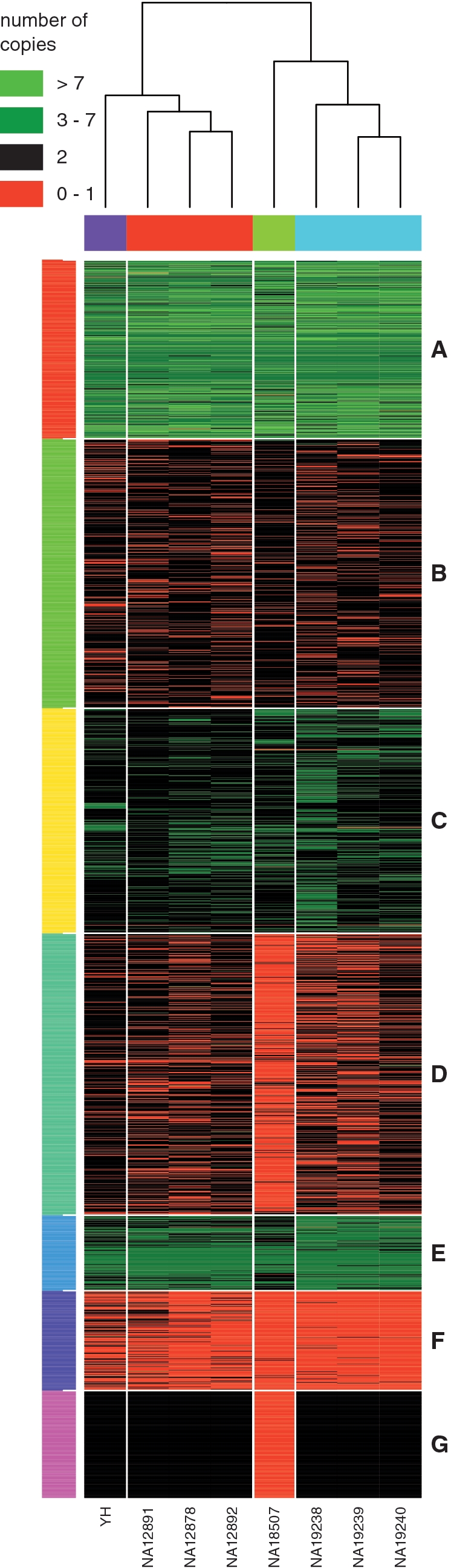
Hierarchical clustering on the estimated copy number of the 3000 CNV regions detected by JointSLM on chromosome 1 with parameters η = 10⁻⁶, ω = 0.1 and K₀ = 20. Each row represents a separate CNVs region and each column a separate individual. The coloured bars on the right of the figure represent clusters of genomic events that share similar CNV patterns over multiple individuals.

The genomic regions grouped in cluster A, E and F contain CNVs with high population frequency (shared among almost all of the eight individuals), while clusters B, C and D contain subgroups of CNVs that are primarily shared among Yoruban ancestry or european ancestry. As expected, the three clusters with common amplifications showed a greater enrichment of annotated SDs compared with the clusters that contain deletions. SDs accounted for 73, 63 and 54% of the total base pairs of clusters A, C and E, while for clusters B, D and F we found an overlap of 29, 31 and 23%, respectively.

Conversely, we observed that the clusters that contain common deletions (B, D and F) showed a greater enrichment of annotated genes compared with the amplification clusters. The number of RefSeq genes that overlap with clusters A, B and C are 128, 151 and 43, while for the deletion clusters D, E and F we found an overlap with 236, 360 and 117 RefSeq genes, respectively.

We also studied the overlap between the CNV regions that belong to each of the seven clusters and annotated regions with SRs: we found that all the clusters have an average overlap of the order of 6–8% with SR events, with the exception of cluster A that have more than 15%. Clusters A contain 434 amplification regions with very complex pattern of CNVs: around 65% of the amplifications that belong to cluster A have an estimated number of copies greater than 4.

DISCUSSION

We developed a novel algorithm that extend the univariate SLM to the multivariate case in order to detect recurrent shifts in the mean of multiple sequential processes. We applied JointSLM to DOC signals obtained from high coverage sequencing data in order to infer common CNVs among multiple individuals.

The results obtained in simulated chromosomes show that JointSLM correctly detects recurrent CNV regions as small as 500 bp in size with sensitivity larger than 90%. The comparison with other state of the art methods demonstrated the our joint model is able to obtain an unprecedented resolution in the analysis of DOC data (see Supplementary Data). We applied our algorithm on chromosome 1 of eight genomes and we identified 3000 regions with recurrent CNVs of different frequency and size. We validated in silico the 3000 CNVs regions by studying the overlap with the annotated CNVs of the Database of Genomic Variants. We found that more than 50% of the inferred regions overlap with annotated CNVs and the validation rate grows up to 70–100% for regions larger than 1 kb. These results clearly show that the use of DOC data combined with our algorithm allows to obtain an unprecedented resolution in the identification of genomic structural variants.

We also demonstrate the utility of JointSLM algorithm for population genetics analysis by applying cluster analysis to the inferred regions. Hierarchical clustering applied to the samples is able to separate the eight individuals in two main clusters that reflects their ancestry, while cluster analysis on the regions allows to identify groups of CNVs that share structural features such as enrichment in segmental duplications, enrichment in simple repeats and gene content.

JointSLM is also able to analyse DOC data from one sample at time obtaining very good results in terms of sensitivity and specificity (see Supplementary Data).

The resolution of JointSLM strictly depends on the signal to noise ratio (SNR) of the data (see ‘Materials and Methods’ section): increasing the SNR of DOC data by reducing the sequencing error rate or augmenting the coverage of the sequencing experiments, will improve the performance of JointSLM in detecting small shifts in the signals.

The JointSLM algorithm can be also used to analyse multiple tumour samples data for the discovery of recurrent copy number alterations. In this case, to estimate DNA copy numbers it is necessary to take into account cellularity and tumoural heterogeneity and for this reason we would need a more sophisticated approach similar to CGHCall (26) or FastCall (27) instead of using the simple rounding to the closest integer. Although all the analyses performed in this article were made on sequence data from the Illumina Genome Analyzer, the algorithm we developed is generic and can be used to analyse DOC data produced by different HTS platforms.

AVAILABILITY

The JointSLM algorithm is implemented as an R package. The source code includes both R and Fortran codes. The JointSLM package and a brief manual is freely available as Supplementary Data.

SUPPLEMENTARY DATA

Supplementary Data are available at NAR Online.

FUNDING

This study was supported by the project “Gene expression profile and therapeutic implication in gastric cancer. From the clinical overview to the translational research” of the Istituto Toscano Tumori (ITT).

Conflict of interest statement. None declared.

REFERENCES

- 1.Feuk L, Carson AR, Scherer SW. Structural variation in the human genome. Nat. Genet. 2006;7:85–97. doi: 10.1038/nrg1767. [DOI] [PubMed] [Google Scholar]
- 2.Tuzun E, Sharp AJ, Bailey JA, Kaul R, Morrison VA, Pertz LM, Haugen E, Hayden H, Albertson D, Pinkel D, et al. Fine-scale structural variation of the human genome. Nat. Genet. 2005;37:727–732. doi: 10.1038/ng1562. [DOI] [PubMed] [Google Scholar]
- 3.Iafrate AJ, Feuk L, Rivera MN, Listewnik ML, Donahoe PK, Qi Y, Scherer SW, Lee C. Detection of large-scale variation in the human genome. Nat. Genet. 2004;36:949–951. doi: 10.1038/ng1416. [DOI] [PubMed] [Google Scholar]
- 4.Redon R, Ishikawa S, Fitch KR, Feuk L, Perry GH, Andrews TD, Fiegler H, Shapero MH, Carson AR, Wenwei Chen W, et al. Global variation in copy number in the human genome. Nature. 2006;444:444–454. doi: 10.1038/nature05329. [DOI] [PMC free article] [PubMed] [Google Scholar]
- 5.Kidd JM, Cooper GM, Donahue WF, Hayden HS, Sampas N, Graves T, Hansen N, Teague B, Alkan C, Antonacci F, et al. Mapping and sequencing of structural variation from eight human genomes. Nature. 2008;453:56–64. doi: 10.1038/nature06862. [DOI] [PMC free article] [PubMed] [Google Scholar]
- 6.McCarroll S, Kuruvilla F, Korn J, Cawley S, Nemesh J, Wysoker A, Shapero M, de Bakker P, Maller J, Kirby A, et al. Integrated detection and population-genetic analysis of SNPs and copy number variation. Nat. Genet. 2008;40:1166–1174. doi: 10.1038/ng.238. [DOI] [PubMed] [Google Scholar]
- 7.McCarroll SA, Altshuler DM. Copy-number variation and association studies of human disease. Nat. Genet. 2007;39:S37–S42. doi: 10.1038/ng2080. [DOI] [PubMed] [Google Scholar]
- 8.Volik S, Zhao S, Chin K, Brebner JH, Herndon DR, Tao Q, Kowbel D, Huang G, Lapuk A, Kuo WL, et al. End-sequence profiling: sequence-based analysis of aberrant genomes. Proc. Natl Acad. Sci. USA. 2003;100:7696–7701. doi: 10.1073/pnas.1232418100. [DOI] [PMC free article] [PubMed] [Google Scholar]
- 9.Raphael BJ, Volik S, Collins C, Pevzner PA. Reconstructing tumor genome architectures. Bioinformatics. 2003;19(Suppl. 2):162–171. doi: 10.1093/bioinformatics/btg1074. [DOI] [PubMed] [Google Scholar]
- 10.Futreal PA, Coin L, Marshall M, Down T, Hubbard T, Wooster R, Rahman N, Stratton MR. A census of human cancer genes. Nat. Rev. Cancer. 2004;4:177–183. doi: 10.1038/nrc1299. [DOI] [PMC free article] [PubMed] [Google Scholar]
- 11.Rovelet-Lecrux A, Hannequin D, Raux G, Le Meur N, Laquerrière A, Vital A, Dumanchin C, Feuillette S, Brice A, Vercelletto M, et al. APP locus duplication causes autosomal dominant early-onset Alzheimer disease with cerebral amyloid angiopathy. Nat. Genet. 2006;38:24–26. doi: 10.1038/ng1718. [DOI] [PubMed] [Google Scholar]
- 12.Singleton AB, Farrer M, Johnson J, Singleton A, Hague S, Kachergus J, Hulihan M, Peuralinna T, Dutra A, Nussbaum R, et al. Alpha-synuclein locus triplication causes Parkinson's disease. Science. 2003;302:841. doi: 10.1126/science.1090278. [DOI] [PubMed] [Google Scholar]
- 13.Cooper GM, Zerr T, Kidd JM, Eichler EE, Nickerson DA. Systematic assessment of copy number variant detection via genome-wide SNP genotyping. Nat. Genet. 2008;40:1199–1203. doi: 10.1038/ng.236. [DOI] [PMC free article] [PubMed] [Google Scholar]
- 14.Medvedev P, Stanciu M, Brudno M. Computational methods for discovering structural variation with next-generation sequencing. Nat. Methods. 2009;6:S13–S20. doi: 10.1038/nmeth.1374. [DOI] [PubMed] [Google Scholar]
- 15.Dalca AV, Brudno M. Genome variation discovery with high-throughput sequencing data. Brief Bioinform. 2010;11:3–14. doi: 10.1093/bib/bbp058. [DOI] [PubMed] [Google Scholar]
- 16.Campbell PJ, Stephens PJ, Pleasance ED, O'Meara S, Li H, Santarius T, Stebbings LA, Leroy C, Edkins S, et al. Identification of somatically acquired rearrangements in cancer using genome-wide massively parallel paired-end sequencing. Nat. Genet. 2008;40:722–729. doi: 10.1038/ng.128. [DOI] [PMC free article] [PubMed] [Google Scholar]
- 17.Olshen AB, Venkatraman ES, Lucito R, Wigler M. Circular binary segmentation for the analysis of array-based DNA copy number data. Biostatistics. 2005;5:557–572. doi: 10.1093/biostatistics/kxh008. [DOI] [PubMed] [Google Scholar]
- 18.Chiang DY, Getz G, Jaffe DB, O'Kelly MJT, Zhao X, Carter SL, Russ C, Nusbaum C, Meyerson M, Lander ES. High-resolution mapping of copy-number alterations with massively parallel sequencing. Nat. Methods. 2009;9:99–103. doi: 10.1038/nmeth.1276. [DOI] [PMC free article] [PubMed] [Google Scholar]
- 19.Yoon S, Xuan Z, Makarov V, Ye K, Sebat J. Sensitive and accurate detection of copy number variants using read depth of coverage. Genome Res. 2009;19:1586–1592. doi: 10.1101/gr.092981.109. [DOI] [PMC free article] [PubMed] [Google Scholar]
- 20.Magi A, Benelli M, Marseglia G, Nannetti G, Scordo MR, Torricelli F. A shifting level model algorithm that identifies aberrations in array-CGH data. Biostatistics. 2010;11:265–280. doi: 10.1093/biostatistics/kxp051. [DOI] [PubMed] [Google Scholar]
- 21.Rabiner LR. A tutorial on hidden Markov models and selected applications in speech recognition. Proc. IEEE. 1988;77:257–286. [Google Scholar]
- 22.Hupè P, Stransky N, Thiery JP, Radawanyi F, Barillot E. Analysis of array-CGH data: from signal ratio to gain and loss of DNA regions. Bioinformatics. 2004;20:3413–3422. doi: 10.1093/bioinformatics/bth418. [DOI] [PubMed] [Google Scholar]
- 23.Bentley DR, Balasubramanian S, Swerdlow HP, Smith GP, Milton J, Brown CG, Hall KP, Evers DJ, Barnes CL, Bignell HR, et al. Accurate whole human genome sequencing using reversible terminator chemistry. Nature. 2008;456:53–59. doi: 10.1038/nature07517. [DOI] [PMC free article] [PubMed] [Google Scholar]
- 24.Wang J, Wang W, Li R, Li Y, Tian G, Goodman L, Fan W, Zhang J, Li J, Zhang J, et al. The diploid genome sequence of an Asian individual. Nature. 2008;456:60–65. doi: 10.1038/nature07484. [DOI] [PMC free article] [PubMed] [Google Scholar]
- 25.Nguyen DQ, Webber C, Ponting CP. Bias of Selection on Human Copy-Number Variants. PLoS Genet. 2006;2:e20. doi: 10.1371/journal.pgen.0020020. [DOI] [PMC free article] [PubMed] [Google Scholar]
- 26.van de Wiel MA, Kim KI, Vosse SJ, van Wieringen WN, Wilting SM, Ylstra B. CGHcall: calling aberrations for array CGH tumor profiles. Bioinformatics. 2007;23:892–894. doi: 10.1093/bioinformatics/btm030. [DOI] [PubMed] [Google Scholar]
- 27.Benelli M, Marseglia G, Nannetti G, Paravidino R, Zara F, Bricarelli FD, Torricelli F, Magi A. A very fast and accurate method for calling aberrations in array-CGH data. Biostatistics. 2010;11:515–518. doi: 10.1093/biostatistics/kxq008. [DOI] [PubMed] [Google Scholar]
Associated Data
This section collects any data citations, data availability statements, or supplementary materials included in this article.