Wave-spec: a preprocessing package for mass spectrometry data

Abstract

Summary:Wave-spec is a pre-processing package for mass spectrometry (MS) data. The package includes several novel algorithms that overcome conventional difficulties with the pre-processing of such data. In this application note, we demonstrate step-by-step use of this package on a real-world MALDI dataset.

Availability: The package can be downloaded at http://www.vicc.org/biostatistics/supp.php. A shared mailbox (wave-spec@vanderbilt.edu) also is available for questions regarding application of the package.

Contact: yu.shyr@vanderbilt.edu

Supplementary information: Supplementary data are available at Bioinformatics online.

1 INTRODUCTION

This paper demonstrates how the Wave-spec package works, as an application note designed to complement a Wave-spec method paper published previously (Chen et al., 2009). The rest of this paper is organized as a step-by-step demonstration on real MALDI-TOF data and follows the procedure presented in Supplementary Figure S1.

2 WAVE-SPEC APPLICATION

Users of Wave-spec must have basic programming skills in Matlab as well as background knowledge on mass spectrometry (MS) data. Given the complexity of high-throughput datasets, it is unrealistic to expect that an inexperienced user would master the use of Wave-spec, even with the thorough guidance outlined here.

2.1 Read in data

For the purpose of demonstration, we chose 210 spectra from one training cohort in a published dataset: 70 patients in ‘Italian A’ with 3 spectra per patient. Details of the data are given in (Taguchi et al., 2007). For a batch read-in, it is best to put all the spectrum files in one folder. For example, we place the data in the following folder and the first command is to give the directory:

In .txt format, each data file should have two columns. The first column is m/z, and the second is intensity. Based on our experience, in most cases, the spectra will have the same acquisition frequency but slightly different m/z values across all samples. The following two commands are used to combine all spectral intensities (denoted as Y) and to provide a common m/z value with the same dimension for all spectra.

It is important to note two other possible situations involving m/z values: (i) all spectra share exactly the same m/z values. In this case, we need only the first command; and (ii) the acquisition frequencies are different, in which case the m/z values exhibit a large discrepancy across all samples (for example, due to being acquired from different machines/institutes). In this case, an interpolation algorithm might be needed to decide a common m/z value.

2.2 Calibration

Calibration is a highly interactive process. First, prior to calibration, we need a candidate calibration peak list, which is typically provided by the investigator. Secondly, we select appropriate peaks from this list by viewing their shape in the data we have [criteria for candidate peak selection are described in (Chen et al., 2009)]. For example, Supplementary Figure S2 shows that 9428 might be a good choice, as are 6631, 11 649.3, and 15 868. Therefore, we use the following commands for spectral calibration.

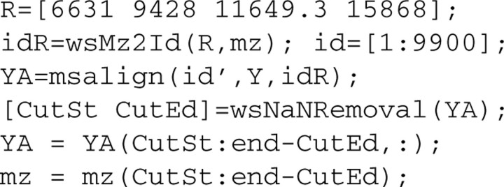
Note that, with the last three lines of code, we ignore some of the starting and ending values of the spectra, to avoid possible N/A values generated by the calibration process at starting and/or ending positions of spectra. The following process is not affected by these missing values. After calibration, we need to check the calibration performance, not only plotting the spectra before and after calibration around the calibration point, but also viewing the overall calibration performance for the full spectral range. For example, Supplementary Figures S2 and S3 show the results before and after calibration around candidate peak 9428. (Note that we generated and viewed additional plots to check the overall calibration performance, without presenting them here.)

2.3 Feature selection

The step after calibration is to extract common features from the spectra. As explained in the initial method paper, the number of ‘peaks’ is determined by the level of wavelet denoising, and an appropriate smoothing threshold is obtained by a feedback index: the ratio of baseline area to total area under the peak location distribution curve. To balance the tradeoff between admitting false peaks and removing true peaks, we apply the following schema. First, we pre-specify the feedback index upper limit (for example, 0.05). Then, we increase the wavelet threshold from relatively low levels until the feedback index is low enough to meet the upper limit constraint. To illustrate the threshold selection process, we set 3 values for the wavelet denoising threshold, thre, and set other parameters with fixed values in the code below.

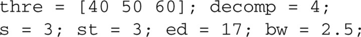
In most cases, the recommended selection range for thre is between 40 and 80. The other key parameters to tune and their recommended ranges are: (i) decomposition level, decomp, [2,3,4]; (ii) spectral intensity signal-to-noise ratio, s, [2 to 4]; (iii) band width, bw, [1 to 3]; and (iv) starting and ending m/z location, st and ed, respectively, [2k to 3k] and [17k to 20k] Dalton. (Note that the above parameter ranges have been successfully applied to most datasets we have analyzed; for any specific project with much tense or loose acquisition frequency, these values might not work and should be adjusted accordingly.) After setting the above parameters, we are ready to calculate the feedback index. The following codes calculate the feedback index and generate Supplementary Figure S4. (Note: inten is peak intensity value, bins provides peak location and range, and snr is the ratio of baseline area to the total area under the peak location distribution curve.)

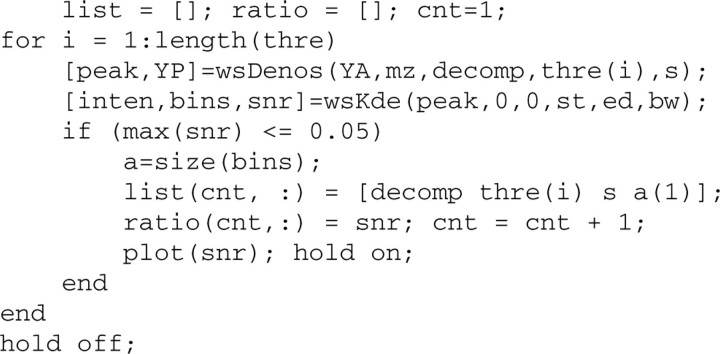
Supplementary Figure S4 shows that when the threshold is set at 60, the feedback index obtains optimal values along the whole spectral range. Such a figure is usually generated to assist on deciding the optimal threshold. We then apply this parameter to achieve the final smoothing.

2.4 Feature quantification

We quantify the selected features by calculating the area under a baseline-corrected (YB) and normalized (YN) curve. The final output intensity for selected features are auc. These steps can be achieved using the following code:

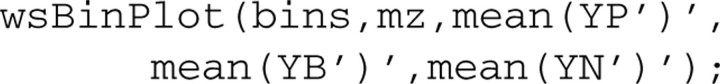
Supplementary Figure S5 provides average curves for the whole m/z range at 3 different pre-processing stages: (i) denoised only; (ii) denoised plus background-corrected; and (iii) denoised, background-corrected and normalized. The identified peaks are contained in rectangles (bins). This plot is helpful when reviewing and verifying pre-processing at the end of the procedure: we expect to see all large peaks contained in bins, and the average curve is smooth without elevated background. (Supplementary Figure S6 is a detailed version of Supplementary Figure S5 for a small m/z range.) Such plots can be obtained using the following code:

2.5 Output results

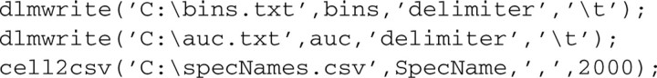
The final step in the procedure is to write out the results or any intermediate values that might be needed for further statistical analysis. For example, for bin range, peak values and names of each spectrum, use the following code to write out results:

3 DISCUSSION AND CONCLUSION

By using a publicly available mass spectrometry dataset, we have demonstrated how Wave-spec works. This package can be applied to many types of MS data, such as direct infusion or flow injection MS data, as well as MALDI-TOF MS reflectron-mode data. A user who wishes to apply our package should adapt our sample code accordingly and refer to the corresponding method paper.

REFERENCES

- Chen S, et al. A novel comprehensive wave-form MS data processing method. Bioinformatics. 2009;25:808–814. doi: 10.1093/bioinformatics/btp060. [DOI] [PMC free article] [PubMed] [Google Scholar]
- Taguchi F, et al. Mass spectrometry to classify non-small-cell lung cancer patients for clinical outcome after treatment with epidermal growth factor receptor tyrosine kinase inhibitors: A multicohort cross-institutional study. J. Natl. Cancer Inst. 2007;99:838–846. doi: 10.1093/jnci/djk195. [DOI] [PubMed] [Google Scholar]
Associated Data
This section collects any data citations, data availability statements, or supplementary materials included in this article.