Variable selection for discriminant analysis with Markov random field priors for the analysis of microarray data

Abstract

Motivation: Discriminant analysis is an effective tool for the classification of experimental units into groups. Here, we consider the typical problem of classifying subjects according to phenotypes via gene expression data and propose a method that incorporates variable selection into the inferential procedure, for the identification of the important biomarkers. To achieve this goal, we build upon a conjugate normal discriminant model, both linear and quadratic, and include a stochastic search variable selection procedure via an MCMC algorithm. Furthermore, we incorporate into the model prior information on the relationships among the genes as described by a gene–gene network. We use a Markov random field (MRF) prior to map the network connections among genes. Our prior model assumes that neighboring genes in the network are more likely to have a joint effect on the relevant biological processes.

Results: We use simulated data to assess performances of our method. In particular, we compare the MRF prior to a situation where independent Bernoulli priors are chosen for the individual predictors. We also illustrate the method on benchmark datasets for gene expression. Our simulation studies show that employing the MRF prior improves on selection accuracy. In real data applications, in addition to identifying markers and improving prediction accuracy, we show how the integration of existing biological knowledge into the prior model results in an increased ability to identify genes with strong discriminatory power and also aids the interpretation of the results.

Contact: marina@rice.edu

1 INTRODUCTION

Discriminant analysis, sometimes called supervised pattern recognition, is a statistical technique used to classify observations into groups. For each case in a given training set a p × 1 vector of observations, x_i, and a known assignment to one of G groups are available. On the basis of these data, we wish to derive a classification rule that assigns future cases to their correct groups. If the distribution of the n × p matrix X of the data, conditional on the group membership, is assumed to be a multivariate normal, then this statistical methodology is known as discriminant analysis.

We consider the typical problem of classifying subjects according to phenotypes via gene expressions and propose a method to include a variable selection procedure into the inferential process, for the identification of the important biomarkers. We build upon a conjugate normal discriminant model, linear or quadratic, and include a stochastic search variable selection procedure via an MCMC algorithm. Furthermore, we use dependent priors that reflect known relationships among the genes. Recently, there has been a rapid accumulation of biological knowledge in the form of various gene–gene networks. The importance of incorporating such biological knowledge into the analysis of genomic data has been increasingly recognized. Here, we view a gene–gene network as an undirected graph with nodes representing genes and edges representing interactions between genes. We capture this information via a Markov random field (MRF) prior that maps the connections among genes. Our prior model assumes that neighboring genes in the network are more likely to have a joint effect on the relevant biological processes. Similar priors have been used in linear regression models by Li and Zhang (2010), Wei and Pan (2010) and Stingo et al. (2010) and in gamma-gamma models by Wei and Li (2007, 2008). We extend their use to the discriminant analysis setting. We illustrate our method for the case of quadratic discriminant analysis, where different groups are allowed to have different covariance matrices.

We show good performances on simulation studies and illustrate the method on benchmark datasets for gene expression. In particular, we compare the MRF prior to a situation where independent Bernoulli priors are chosen for the individual predictors and show that employing the MRF prior leads to more accurate selection. Other authors have reported similar results. Li and Zhang (2010), in particular, comment on the effect of the MRF prior on the selection power in their linear regression setting. They also notice that adding the MRF prior implies a relatively small increase in computational cost. Wei and Li (2007, 2008) and Stingo et al. (2010) report that their methods are quite effective in identifying genes and modified subnetworks, with higher sensitivity than commonly used procedures that do not use the network structure, and similar or, in some cases, lower false discovery rates. In real data applications, in addition to improving prediction accuracy, we show how the integration of biological knowledge into the prior model results in an increased ability to identify genes with strong discriminatory power and also aids the interpretation of the results.

The rest of the article is organized as follows: in Section 2, we introduce discriminant analysis under the Bayesian paradigm and describe how to perform variable selection. We also propose a way to incorporate information about gene–gene networks into the prior model. In Section 3, we present the MCMC algorithm for posterior inference. In Section 4, we investigate performances of the proposed method on simulated data and conclude, in Section 5, with applications to benchmark datasets for gene expression where we incorporate the gene–gene network prior.

2 BAYESIAN DISCRIMINANT ANALYSIS

Let X indicate the observed data and let y be the n × 1 vector of group indicators. We assume that each observation comes from one of G possible groups, each with distribution N(μ_g, Σ_g). We represent the data from each group by the n_g × p matrix

(1)

with g = 1,…, G and where the vector μ_g and the matrix Σ_g are the mean and the covariance matrix of the g-th group, respectively. Here the notation V − M ∼ 𝒩(A, B) indicates a matrix normal variate V with matrix mean M and with variance matrices b_iiA for its generic i-th column and a_jjB for its generic j-th row, see Dawid (1981). Taking a conjugate Bayesian approach, we impose a multivariate normal distribution on μ_g and an inverse-Wishart prior on the covariance matrix Σ_g, that is,

This parametrization, besides being the standard setting in Bayesian inference, allows us to create a computationally efficient variable selection algorithm by integrating out means and covariances and designing Metropolis steps that depend only on the selected and proposed variables, see Section 3.

In discriminant analysis, the predictive distribution of a new observation x^f is used to classify the new sample into one of the possible G groups. This distribution, see Brown (1993) among others, is a multivariate T-student of the type

(2)

where , δ_g^* = δ_g +n_g, a_g = 1 + (1/h_g + n_g)⁻¹ and with π_g = (1 + h_gn_g)⁻¹ and .

The probability that the future observation, given the observed data, belongs to group g is then given by

(3)

where y^f is the group indicator of the new observation. By estimating the prior probability that one observation comes from group g with , the previous distribution can be written in closed form as

where p_g(X^f) indicates the predictive distribution defined in (2). The new observations is then assigned to the group with the highest posterior probability.

2.1 Likelihood and prior setting for variable selection

Our aim is to construct a classifier while simultaneously selecting the discriminating variables (i.e. biomarkers). Here, we extend an approach to variable selection proposed by Tadesse et al. (2005) for model-based clustering to the discriminant analysis framework. As done by these authors, we introduce a (p × 1) latent binary vector γ, whose elements equal to 1 indicate the selected variables, i.e. γ_j = 1 if variable j contributes to the classification of the n units into the corresponding groups. We use the latent vector γ to index the contribution of the different variables to the likelihood. Unlike Tadesse et al. (2005), we avoid any independent assumption among the variables by defining a likelihood that allows to separate the discriminating variables from the noisy ones as

(4)

where w_g is the prior probability that unit i belongs to group g, X_i(γ^c) is the |γ^c| × 1 vector of the non−selected variables and X_i(γ) is the |γ| × 1 vector of the selected ones, for the i-th subject. Under the normality assumption on the data, the likelihood becomes

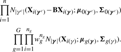where B is a matrix of regression coefficients resulting from the implied linearity of the expected value of the conditional distribution p(X_i(γ^c)|X_i(γ)), and where μ_0(γ^c) and Σ_0(γ^c) are the mean and covariance matrix, respectively, of X_i(γ^c). Murphy et al. (2010) use the same likelihood factorization (4) in a frequentist approach to variable selection in discriminant analysis. We again impose conjugate priors on the parameters corresponding to the non-selected variables:

We complete the prior model by defining an improper non-informative prior on the vector w = (w₁,…, w_G) as a Dirichlet distribution, w ∼ Dirichlet(0,…, 0). We discuss priors for the latent indicator γ in the next Section. Note that, with the inclusion of the variable selection mechanism, the predictive distribution (3) does not change as it depends only on the selected variables.

Without loss of generality, at least for the inferential procedure described in Section 3, we can assume that the set of non-selected variables is formed by only one variable so that the prior parametrization can be simplified using the scalar σ² instead of Σ_0(γ^c) and the (|γ| × 1) vector β instead of the |γ^c| × |γ| matrix B, with σ² ∼ Inv − Gamma(δ/2, k_0/2) and β ∼ N(β₀, σ²H_γ). To obtain this parametrization, the commonly used assumption Ω_0(γ^c) = k₀I_|γ^c| is needed, see for example Tadesse et al. (2005) for a model-based clustering context, and Dobra et al. (2004) for a graphical model context.

2.2 Prior distribution for the integration of gene network information

Although the model allows for dependencies among the variables, it is not straightforward to specify dependence structures known a priori on the covariance matrix prior. When prior information is available, a better strategy is to incorporate it into the prior distribution on γ. The prior model for this parameter is indeed quite flexible and allows the incorporation of biological information in a very natural way. Here, we use in particular biological information that derive from existing databases on gene–gene networks. We encode such gene–gene network information in our model via a MRF prior on γ. A MRF is a graphical model in which the distribution of a set of random variables follows Markov properties that can be described by an undirected graph.

In our context, the MRF structure represents the gene–gene network, i.e. genes are represented by nodes and relations between them by edges (direct links). With the parametrization we adopt the global MRF distribution for γ is given by

(5)

with d = d1_p and 1_p the unit vector of dimension p, and F a matrix with elements {f_ij} usually set to some constants f for the connected nodes and to 0 for the non-connected ones. Here d controls the sparsity of the model, while f affects the probability of selection of a variable according to its neighbor values. This is more evident by noting that the conditional probability

(6)

with N_j the set of direct neighbors of variable j in the MRF, increases as a function of the number of selected neighbor genes. With this parametrization, some care is needed in deciding whether to put a prior distribution on f. Allowing f to vary can in fact lead to a phase transition problem, that is, the expected number of variables equal to 1 can increase massively for small increments of f. This problem can happen because Equation (6) can only increase as a function of the number of x_j's equal to 1.

If a variable does not have any neighbor, its prior distribution reduces to an independent Bernoulli with parameter p = exp(d)/[1 + exp(d)], which is a logistic transformation of d.

3 MCMC FOR POSTERIOR INFERENCE

With the main purpose being variable selection, we perform posterior inference by concentrating on the posterior distribution on γ. This distribution cannot be obtained in closed form and an MCMC is required. The inferential procedure can be simplified by integrating out the parameters w_g, β, σ², μ₀, μ_g and Σ_g, obtaining the following marginal likelihood:

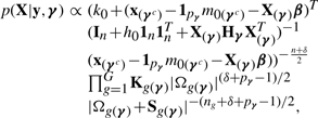where

We implement a Stochastic Search Variable Selection (SSVS) algorithm that has been successfully and extensively used in the variable selection literature, see Madigan and York (1995) for graphical models, Brown et al. (2002) for linear regression models, Sha et al. (2004) for classification settings with probit models and Tadesse et al. (2005) for clustering, among others. This is a Metropolis type of algorithm that uses two types of move, the addition/deletion of one selected variable or the swapping of one selected variable with a non selected one, as follows:

• with probability ϕ, add or delete one variable by choosing at random one component in the current γ and changing its value;

• with probability 1 − ϕ, swap two elements by choosing independently at random one 0 and one 1 in the current γ and changing their values.

The proposed γ^new is accepted with probability given by the ratio of the relative posterior probabilities of new versus current model

(7)

Because these moves are symmetric, the proposal distribution does not appear in the ratio above. In addition, the calculation of (7) can be simplified using a factorization of the marginal likelihood that allows to treat the part that involves the non-significant variables as one-dimensional, see Murphy et al. (2010) for the full details.

The MCMC procedure results in a list of visited models, γ⁽⁰⁾,…, γ^(T) and their corresponding posterior probabilities. Variable selection can then be achieved either by looking at the γ vectors with largest joint posterior probabilities among the visited models or, marginally, by calculating frequencies of inclusion for each γ_j and then choosing those γ_j's with frequencies exceeding a given cut-off value. Finally, using the selected variables new observations are assigned to one of the G groups according to (3).

4 SIMULATED DATA

We first validate our approach through simulations. We consider simulated scenarios that mimic the characteristics of gene expression data, in particular the relatively small sample size with respect to the number of variables and the fact that variables exhibit correlation structure. We focus on situations where most of the variables are noisy ones, to test the ability of our method to discover relevant covariates in the presence of a good amount of noise.

More in details, we generated a sample of 50 observations from a mixture of three multivariate normal densities, induced by six variables,

with x_i = (x_i,1,…, x_i,6), for i = 1,…, 50, and where I_[.] is the indicator function. The first 20 samples arose from the first distribution, the next 15 came from the second group and the last 15 from the third group. We then divided the observations into two sets, obtaining a training set of size 33 and a validation set of size 17. The training set was formed by 13 units from group 1, 10 from group 2 and 10 from group 3 while the validation set by 7 units from group 1, 5 from group 2 and 5 from group 3. We set the means of the normal distributions equal to μ₁ = −2 × 1_p, μ₂ = 3.5 × 1_p and μ₃ = 1 × 1_p, where 1_p is a unit vector of dimension p = 6. We constructed the covariance matrices of the six variables in the following way: the elements on the diagonals were set to σ²₁ = 3, σ²₂ = 2 and σ²₃ = 2.5. The correlation structures of the six variables were then represented by 3 × 2 grids with elements equal to 0.2 if two variables were connected and 0 otherwise. We arbitrarily connected each variable in the 3 × 2 lattice systems to either 2 or 3 other variables. This generating mechanism creates correlation also between variables not directly connected in the lattice systems.

We report here results obtained by considering four different settings: in settings (i) and (ii) an additional set of s = 100 noisy variables was generated. Settings (iii) and (iv) used 1024 noisy variables. The noisy variables were generated using a linear regression model where each of the six discriminatory variables affected three noisy variables and where the covariance structure of the error terms corresponded to a 10 × 10 (or 33 × 32) lattice system with correlations equal to 0.1 and variances set to 1 for settings (i) and (iii) and 2 for settings (ii) and (iv). This generating mechanism produced the following empirical correlation: in setting (i) the correlations between the noisy variables were in the range (−0.42, 0.54), those between the discriminatory variables were in the range (0.55, 0.80) and those between the noisy variables and the discriminatory ones in (−0.39, 0.59). In setting (ii), the correlations between the noisy variables were in the range (−0.42, 0.54), those between the discriminatory variables in (0.55, 0.80) and those between the noisy variables and the discriminatory ones in (−0.39, 0.50). In setting (iii), the correlations between the noisy variables were in the range (−0.60, 0.59), those between the discriminatory variables in (0.55, 0.80) and between the noisy variables and the discriminatory ones in (−0.52, 0.70). Finally, in setting (iv) the correlations between the noisy variables were in the range −0.60, 0.59, those between the discriminatory variables in (0.55, 0.80) and those between the noisy variables and the discriminatory ones in (−0.52, 0.64). In every setting, we permuted the columns of the data matrix X, to disperse the predictors.

We set δ = 3, the minimum value such that the expectation of Σ exists, and, as suggested by Tadesse et al. (2005), specified H_γ = 100 · I_|γ|, h₁ = … = h_G = 10, h₀ = 100 to obtain priors fairly flat over the region where the data are defined. Some care is needed in the choice of Ω_g and k₀. As suggested by Kim et al. (2006), these hyperparameters should be specified in the range of variability of the data. We found that a value around the mean of the first l eigenvalues of the covariance matrix of the data, with l the expected number of significant variables, led to good results. We set Ω_g = 0.05⁻¹ · I_|γ| and k₀ = 10⁻⁴, a value close to the mean of the remaining p − l eigenvalues, and assumed unequal covariances across the groups.

In an effort to show the advantages of using the MRF prior described in Section 2.2, we repeated the analysis of the four scenarios twice, the first time using the MRF prior with f = 1 and the second time using a simple Bernoulli prior on γ. We set the expected number of included variables to 10. For each setting, we ran one MCMC chain for 100 000 iterations, with 10 000 sweeps as burn-in. Each chain started from a model with 10 randomly selected variables. In our Matlab implementation, the MCMC algorithm runs in only 9–11 minutes, depending on the scenario, on an Intel Core 2 Quad station (2.4 GHz) with 4 GB of RAM.

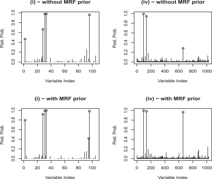
Our results suggest that the MRF prior helps in the selection of the correct variables: in all four scenarios, the posterior probabilities of the discriminatory variables are higher when the MRF prior is used. In addition, some of the discriminatory variables are not selected when the MRF prior is not used. Figure 1, in particular, shows plots of the marginal posterior probabilities of inclusion of single variables, p(γ_j = 1 |X, y), for two of the simulated scenarios. In setting (i) with the MRF prior, a threshold of 0.5 on the posterior probability results in the selection of five of the six significant variables, while a perfect selection is achieved with a threshold of 0.4. Without the MRF prior, a threshold of 0.5 on the posterior probability results in the selection of only four significant variables, while five discriminatory variables are selected with a threshold of 0.4. When calculating the posterior probabilities of class memberships for the 17 observations of the validation set, based on the selected variables, our method perfectly assigns units to the correct groups when the MRF prior is used, while unit 6 is missclassified if this prior is not used. A similar behavior was observed in scenario (ii).

Fig. 1.

Marginal posterior probabilities of inclusion for single variables for two of the four simulated scenarios, with and without MRF prior.

The method performed well also when increasing the number of noisy variables to 1024, with the only difference that the posterior probabilities were generally lower. In setting (iii), using the MRF prior we obtained a perfect selection of all six significant variables with a threshold of 0.19 on the marginal of p(γ_j = 1|X, y), without any false positives. Without MRF prior, the best selection was obtained with a threshold of 0.14 and led to the selection of five of the six significant variables. A threshold of 0.5 led to the selection of four of the six discriminatory variables, both with and without the MRF prior, while a threshold of 0.4 led to the selection of five of the six discriminatory variables when the MRF prior is used and to the selection of four of the six discriminatory variables without the MRF prior. In the most difficult simulation scenario, setting (iv), with a threshold of 0.5 the algorithm with the MRF prior selected three significant variables without any false positive, while when the MRF is not used a threshold of 0.5 led to correctly select two significant variables, without any false positives. A third discriminatory variable was included with a threshold of 0.28.

5 BENCHMARK DATASETS

In this section, we use benchmark examples for gene expression analysis to highlight the characteristics of our proposed method. We focus in particular on performances of the MRF prior (5).

We first analyze the widely used leukemia data of Golub et al. (1999) that comprises a training set of 38 patients and a validation set of 34 patients. The training set consists of bone marrow samples obtained from acute leukemia patients while the validation set consists of 24 bone marrow samples and 10 peripheral blood samples. The aim of the analysis is to identify genes whose expression discriminate acute lymphoblastic leukemia (ALL) patients form acute myeloid leukemia (AML) patients. Following Dudoit et al. (2002), we truncated expression measures beyond the threshold of reliable detection at 100 and 16 000, and removed probe sets with intensities such that max–min ≤ 5 and max–min ≤ 500. This left us with 3571 genes for the analysis. Expression readings were log-transformed and each variable was rescaled by its range. Because of the distributional assumptions behind discriminant analysis, in real data applications it is a good practice to check for normality of the data and apply appropriate transformations, see for example Jafari and Azuaje (2006), among others.

The results we report here were obtained by specifying an MRF prior model of type (5) on γ that uses the gene network structure downloaded from the public available data base KEGG. The network structure was obtained using the R package KEGGgraph of Zhang and Wiemann (2009). All the 3571 probes were included in the analysis. Note that some of the genes do not have neighbors. In our analysis, we assumed that the non-significant variables are marginally independent of the significant ones. We also set the hyperparameters to δ = 3, H_γ = 100 · I_|γ|, h₁ = … = h_G = 10, h₀ = 100, Ω₁ = 0.6⁻¹ · I_|γ| and k₀ = 10⁻¹. This setting is similar to what used in Kim et al. (2006), who analyzed the same dataset using a mixture model for cluster analysis. As for the hyperparameters of the MRF prior, parameterized according to Equation (6), we set d = −2.5 and f = 0.5. The choice of d, in particular, reflects our prior expectation about the number of significant variables, in this case set equal to 7.5% of the total genes analyzed, while a moderate value was chosen for f to avoid the phase transition problem. Two samplers were started with randomly selected starting models that had 10 and 2 included variables, respectively. We ran 150 000 iterations with the first 50 000 used as burn-in. We assessed concordance of the two chains by looking at a scatter plot of the marginal posterior probabilities p(γ_j = 1 |X, y) across the two MCMC chains (Figure not shown) and at the correlation coefficients between these probabilities (r = 0.95).

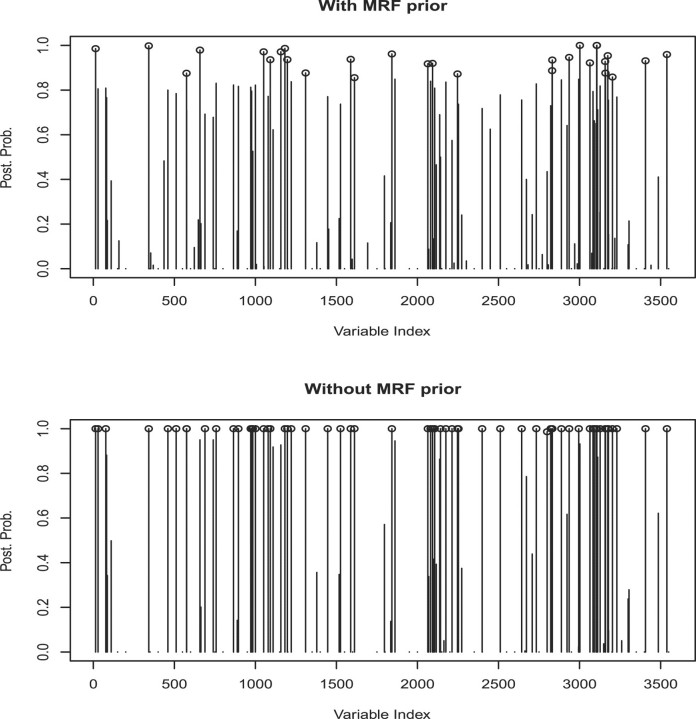
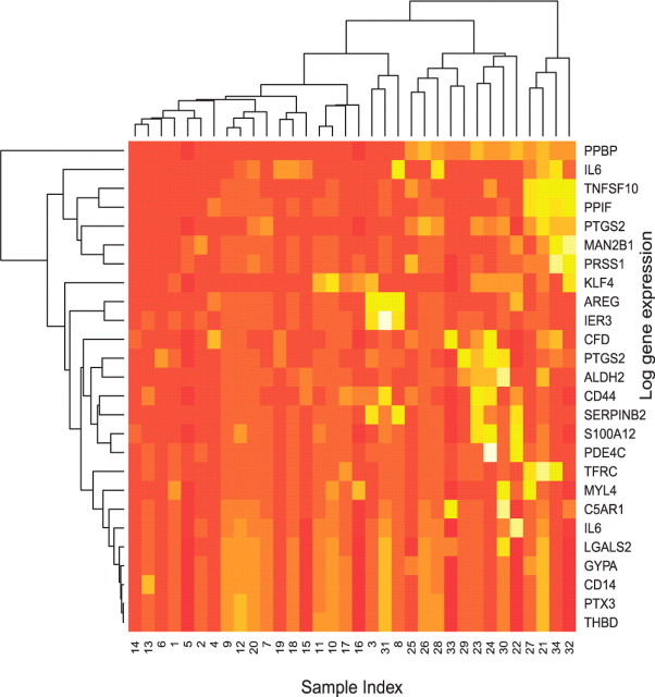
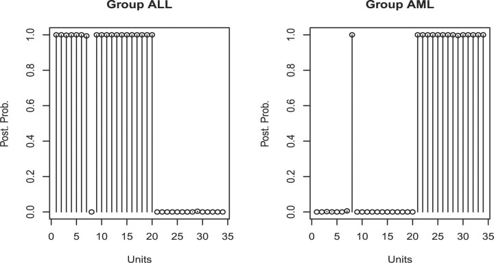
Results we report here were obtained by pooling the outputs from the two chains together. Figure 2 shows the marginal posterior probabilities of inclusion of single genes according to the pooled MCMC output. A threshold of 0.85 on the marginal probability of inclusion resulted in 29 selected genes. A heatmap of the 29 selected genes is given in Figure 3. This figure shows that the selected genes are able to separate the ALL patients, indexed from 1 to 20, from the AML patients, indexed from 21 to 34, with the only exception of unit 31. Indeed, the unsupervised clustering analysis represented by the dendrogram on top of Figure 3 creates a group formed by the entire set of ALL patients, plus unit 31, and other two groups formed by only AML patients, confirming that the 29 selected genes have a very good discriminatory power. In addition, Figure 4 shows the posterior probabilities of class memberships for the 34 units of the validation set, calculated based on the 29 selected genes. According to these probabilities, 33 of the 34 samples were corrected classified.

Fig. 2.

Golub data: marginal posterior probabilities of inclusion for single genes, with and without MRF prior.

Fig. 3.

Golub data: heatmap of the 29 selected genes with a dendrogram of the clustering on the observations (on top) and a dendrogram of the clustering on the selected genes (on the left-hand side).

Fig. 4.

Golub data: posterior probabilities of group memberships for the 34 observations in the validation set.

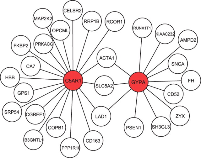
An innovative feature of our method relies in the employment of the MRF field prior. When applying our model without the MRF prior, we noticed a slight decrease in the classification power. In particular, a threshold of 0.95 resulted in 63 selected genes, as shown in Figure 2, and in the correct classification of 30 of the 34 patients of the validation set. Of the 29 genes selected with the MRF field, 26 were included in the set of 63 selected without MRF prior. This result indicates that using information on gene networks, as captured by our MRF prior, leads to an increased ability to identify genes with strong discriminatory power. Additional insights on the selected genes can be found by looking at the prior network. For example, Figure 5 shows the subnetwork of the KEGG network we used that includes the selected genes C5AR1 and GYPA. We notice that the two selected genes appear to be both connected to a same set of genes, including ACTA1, SLC5A2 and LAD1. Such information can be valuable for the biological interpretation of the selection results.

Fig. 5.

Golub data: subnetwork that includes two of the selected genes (in red). Genes are labeled with their gene symbols.

Some of the genes selected by our method are known to be implicated with the differentiation or progression of leukemia cells. For example, Secchiero et al. (2005) have found that cyclooxygenase-2 (with corresponding gene symbol PTGS2), selected by our method with posterior probability of 0.93, increases tumorigenic potential by promoting resistance to apoptosis. Also, Chien et al. (2009) have highlighted the pathogenic role of the vascular endothelial growth factor (VEGF)-C, a recognized tumor lymphangiogenic factor, in leukemia via regulation of angiogenesis through upregulation of cyclooxygenase-2. Peterson et al. (2007) have found that CD44 gene, selected with posterior probability of 0.98, is involved in the growth and maintenance of the AML blast/stem cells. Jin et al. (2006), who studied the mechanisms underlying the elimination of leukemic stem cells (LSCs), also identified CD44 as a key regulator of AML LSCs. Moreover, gene CyP3 (corresponding symbol PPIF) and gene Adipsin (corresponding symbol CFD), selected with posterior probability of 0.97 and 0.99, respectively, were also selected in the original analysis of Golub et al. (1999).

Next we analyzed the data from Alon et al. (1999) on colon cancer, another benchmark for gene expression analysis. We split the 40 tumor and 22 normal colon tissues into a training set of 47 units and a validation set of 15 units. All gene expression profiles were log-10 transformed and standardized to zero mean and unit variance. We again downloaded the gene network structure from the public available data base KEGG using the R package KEGGgraph. We ran two chains from different initial points and then pooled together the visited models. We set δ = 3, H_γ = 100 · I_|γ|, h₁ = … = h_G = 100, h₀ = 10, Ω_g = 0.5⁻¹ · I_|γ| and k₀ = 10⁻³. For the MRF prior, we set f = 1 and the expected number of included variables equal to 10. We assumed unequal covariances across the groups.

Using a threshold of 0.45, we selected 10 genes that were able to correctly classify all the units of the validation set. Most of the 10 selected genes are known to be implicated with the development of colorectal cancer. For example, Wincewicz et al. (2007) found that BCL2-like 1 (BCL2L1), selected by our method with posterior probability 0.79, is of prognostic significance in colorectal cancer. Gulubova et al. (2010) reported that transforming growth factor beta receptor II gene (TGFBR2), selected with posterior probability 0.46, is expressed in tumor cell membranes of colorectal cancers and Ogino et al. (2007) found that this gene is mutated in most microsatellite instability-high (MSI-H) colorectal cancers. When we repeated the analysis without the MRF prior, the algorithm selected a set of 10 genes that correctly classified 14 out 15 samples. The two sets of 10 genes, selected with and without MRF, respectively, shared only a single gene.

The two benchmark datasets we have analyzed have been extensively studied in the literature and similar prediction results have been obtained by other classification methods. For example, in their paper Golub et al. (1999) used the 50 most correlated genes to build a class predictor that incorrectly classified 5 out of the 34 samples of the test set. Dettling (2004) reports comparative results on a number of datasets, including the two we have analyzed, using several classification methods, including Boosting, random forest, support vector machine, nearest neighbor clustering and diagonal linear discriminant analysis. For his analyses, he reports the average misclassification rate calculated over 50 random splits. For the colon cancer dataset, for example, the misclassification rate achieved is around 15%, with DLDA achieving a best rate of 12.9%. To make a more direct comparison with the results obtained by Dettling (2004), we ran our Bayesian algorithm, with the MRF prior, 50 times, using different splits of the data. Following Dettling (2004), we assigned two-thirds of the samples to the training set and one-third to the validation set. Multiple holdout runs are not commonly adopted in Bayesian modeling, due to the impossibility of specifying the hyperparameters on a case-by-case and, in our case, to the difficulty of setting a selection criterion. With the same specification setting across all 50 splits, we obtained misclassification rates that were remarkably similar to the best techniques used in Dettling (2004). For the Leukemia dataset, we achieved an average misclassification rate of 3.9%. With the exception of only one case, where 3 units of the validation set were misclassified, the method correctly classified at least 22 out of 24 samples, with 17 of the 50 splits achieving perfect classification. For the colon cancer dataset, the average misclassification rate was 16.4%.

6 CONCLUSION

We have illustrated how to perform variable selection in discriminant analysis following the Bayesian paradigm. In particular, we have considered the typical problem of classifying subjects according to phenotypes via gene expression data and have proposed prior models that incorporate information on the network structure of genes. Our method allows the classification of future samples and the simultaneous identification of the important biomarkers. Our simulation studies have shown that employing the MRF prior improves on selection accuracy. In applications to benchmark gene expression datasets, we have found that the integration of existing biological knowledge into the prior model results in an increased ability to identify genes with strong discriminatory power and aids the interpretation of the results, in addition to improving prediction accuracy.

Funding: NIH-NHGRI (grant number R01-HG003319); NSF-DMS (grant number 1007871) to M.V. in part.

Conflict of Interest: none declared.

REFERENCES

- Alon U., et al. Broad patterns of gene expression revealed by clustering analysis of tumor and normal colon tissues probed by oligonucleotide arrays. Proc. Natl Acad. Sci. USA. 1999;96:6745–6750. doi: 10.1073/pnas.96.12.6745. [DOI] [PMC free article] [PubMed] [Google Scholar]
- Brown P. Measurement, Regression, and Calibration. Oxford: Oxford University Press; 1993. [Google Scholar]
- Brown P.J., et al. Bayes model averaging with selection of regressors. J. Roy. Stat. Soc. Ser. B. 2002;64:519–536. [Google Scholar]
- Chien M., et al. Vascular endothelial growth factor-c (vegf-c) promotes angiogenesis by induction of cox-2 in leukemic cells via the vegf-r3/jnk/ap-1 pathway. Carcinogenesis. 2009;30:2005–2013. doi: 10.1093/carcin/bgp244. [DOI] [PubMed] [Google Scholar]
- Dawid A.P. Some matrix-variate distribution theory: notational considerations and a Bayesian application. Biometrika. 1981;68:265–274. [Google Scholar]
- Dettling M. Bagboosting for tumor classification with gene expression data. Bioinformatics. 2004;20:3583–3593. doi: 10.1093/bioinformatics/bth447. [DOI] [PubMed] [Google Scholar]
- Dobra A., et al. Sparse graphical models for exploring gene expression data. J. Multivar. Anal. 2004;90:196–212. [Google Scholar]
- Dudoit S., et al. Comparison of discrimination methods for the classification of tumors using gene expression data. J. Am. Stat. Assoc. 2002;97:77–87. [Google Scholar]
- Golub T., et al. Molecular classification of cancer: class discovery and class prediction by gene expression monitoring. Science. 1999;286:531–537. doi: 10.1126/science.286.5439.531. [DOI] [PubMed] [Google Scholar]
- Gulubova M., et al. Role of tgf-beta1, its receptor tgfbetarii, and smad proteins in the progression of colorectal cancer. Int. J. Colorectal Dis. 2010;25:591–599. doi: 10.1007/s00384-010-0906-9. [DOI] [PubMed] [Google Scholar]
- Jafari P., Azuaje F. An assessment of recently published gene expression data analyses: reporting experimental design and statistical factors. BMC Med. Inform. Decis. Mak. 2006;6:27. doi: 10.1186/1472-6947-6-27. [DOI] [PMC free article] [PubMed] [Google Scholar]
- Jin L., et al. Targeting of cd44 eradicates human acute myeloid leukemic stem cells. Nat. Med. 2006;12:1167–1164. doi: 10.1038/nm1483. [DOI] [PubMed] [Google Scholar]
- Kim S., et al. Variable selection in clustering via Dirichlet process mixture models. Biometika. 2006;93:877–893. [Google Scholar]
- Li F., Zhang N. Bayesian variable selection in structured high-dimensional covariate space with application in genomics. J. Am. Stat. Assoc. 2010 to appear. [Google Scholar]
- Madigan D., York J. Bayesian graphical models for discrete data. Int. Stat. Rev. 1995;63:215–232. [Google Scholar]
- Murphy T., et al. Variable selection and updating in model-based discriminant analysis for high dimensional data with food authenticity applications. Ann. Appl. Stat. 2010;4:396–421. doi: 10.1214/09-AOAS279. [DOI] [PMC free article] [PubMed] [Google Scholar]
- Ogino S., et al. Tgfbr2 mutation is correlated with cpg island methylator phenotype in microsatellite instability-high colorectal cancer. Hum. Pathol. 2007;38:614–620. doi: 10.1016/j.humpath.2006.10.005. [DOI] [PubMed] [Google Scholar]
- Peterson L., et al. The multi-functional cellular adhesion molecule cd44 is regulated by the 8;21 chromosomal translocation. Leukemia. 2007;21:2010–2019. doi: 10.1038/sj.leu.2404849. [DOI] [PubMed] [Google Scholar]
- Secchiero P., et al. Potential pathogenetic implications of cyclooxygenase-2 overexpression in b chronic lymphoid leukemia cells. Am. J. Pathol. 2005;167:1559–1607. doi: 10.1016/S0002-9440(10)61244-8. [DOI] [PMC free article] [PubMed] [Google Scholar]
- Sha N., et al. Bayesian variable selection in multinomial probit models to identify molecular signatures of disease stage. Biometrics. 2004;60:812–819. doi: 10.1111/j.0006-341X.2004.00233.x. [DOI] [PubMed] [Google Scholar]
- Stingo F., et al. Incorporating biological information into linear models: a bayesian approach to the selection of pathways and genes. Ann. Appl. Stat. 2010 doi: 10.1214/11-AOAS463. Revised. [DOI] [PMC free article] [PubMed] [Google Scholar]
- Tadesse M., et al. Bayesian variable selection in clustering high-dimensional data. J. Am. Stat. Assoc. 2005;100:602–617. [Google Scholar]
- Wei Z., Li H. A Markov random field model for network-based analysis of genomic data. Bioinformatics. 2007;23:1537–1544. doi: 10.1093/bioinformatics/btm129. [DOI] [PubMed] [Google Scholar]
- Wei Z., Li H. A hidden spatial-temporal markov random field model for network-based analysis of time course gene expression data. Ann. Appl. Stat. 2008;2:408–429. [Google Scholar]
- Wei P., Pan W. Network-based genomic discovery: application and comparison of markov random-field models. Appl. Stat. 2010;59:105–125. doi: 10.1111/j.1467-9876.2009.00686.x. [DOI] [PMC free article] [PubMed] [Google Scholar]
- Wincewicz A., et al. Significant coexpression of glut-1, bcl-xl, and bax in colorectal cancer. Ann. N.Y. Acad. Sci. 2007;1095:53–61. doi: 10.1196/annals.1397.007. [DOI] [PubMed] [Google Scholar]
- Zhang J., Wiemann S. KEGGgraph: a graph approach to KEGG PATHWAY in R and Bioconductor. Bioinformatics. 2009;25:1470–1471. doi: 10.1093/bioinformatics/btp167. [DOI] [PMC free article] [PubMed] [Google Scholar]