Improved similarity scores for comparing motifs

Abstract

Motivation: A question that often comes up after applying a motif finder to a set of co-regulated DNA sequences is whether the reported putative motif is similar to any known motif. While several tools have been designed for this task, Habib et al. pointed out that the scores that are commonly used for measuring similarity between motifs do not distinguish between a good alignment of two informative columns (say, all-A) and one of two uninformative columns. This observation explains why tools such as Tomtom occasionally return an alignment of uninformative columns which is clearly spurious. To address this problem, Habib et al. suggested a new score [Bayesian Likelihood 2-Component (BLiC)] which uses a Bayesian information criterion to penalize matches that are also similar to the background distribution.

Results: We show that the BLiC score exhibits other, highly undesirable properties, and we offer instead a general approach to adjust any motif similarity score so as to reduce the number of reported spurious alignments of uninformative columns. We implement our method in Tomtom and show that, without significantly compromising Tomtom's retrieval accuracy or its runtime, we can drastically reduce the number of uninformative alignments.

Availability and Implementation: The modified Tomtom is available as part of the MEME Suite at http://meme.nbcr.net.

Contact: uri@maths.usyd.edu.au; e.tanaka@maths.usyd.edu.au

Supplementary Information: Supplementary data are available at Bioinformatics online.

1 INTRODUCTION

Research into gene regulation has motivated significant interest in the bioinformatics community in the computational problem of motif finding (Das and Dai, 2007). Consequently, numerous tools have been developed to identify motifs given a set of co-regulated sequences (Tompa et al., 2005).

More recently, the growth of motif databases such as JASPAR (Portales-Casamar et al., 2010), TRANSFAC (Wingender et al., 2000) and a protein-binding microarray (PBM) motif database (Newburger and Bulyk, 2009) spurred the development of new tools designed to allow researchers to test whether the motif returned by a motif finder is ‘significantly similar’ to a known motif [e.g. STAMP, Mahony and Benos (2007) and Tomtom, Gupta et al. (2007)]. Such motif search tools may be viewed as ‘BLAST for motifs’, and their utility includes identification of newly detected motifs and automatic clustering of transcription factor into motif families.

Motif search tools can potentially represent each motif in a variety of ways. The most detailed representation consists simply of the complete list of known binding sites. While useful in some cases, this representation is difficult to work with. At the other extreme is the consensus sequence representation, which often glosses over important subtleties of the motif. Motif database search tools, therefore, typically use a position weight matrix (PWM) representation of the motif. The PWM is typically a 4× l matrix where l is the length of the motif and the (i, j) entry of the matrix contains either the frequency or, alternatively, the count of letter i at position/column j.

After selecting a motif representation, one of the first steps in designing a motif database search tool is the choice of a distance or similarity function between motifs. To the best of our knowledge, all current tools use a linear similarity function which sums up the similarities between the aligned columns of the two motifs. Gupta et al. (2007) performed a comprehensive study comparing the most popular column similarity functions. Their finding was that while generally there are very small differences between most of these functions, the Euclidean distance (ED, Section 7.1 in Supplementary Material) consistently gives slightly better results than the other measures.

Habib et al. (2008) made the important observation that ED, as well as most other scores that are commonly used for measuring similarity between motifs, does not distinguish between alignments of columns with identical composition. For example, the ED score assigns the same perfect score to the two pairs of column alignments in Figures 1A and Figures 1B. Due to the linearity of the score, it follows that the alignments in Figures 1C and Figures 1D also share the same score, even though one is clearly more informative than the other. This is not merely a theoretical issue. Indeed, we have observed that Tomtom occasionally includes clearly spurious alignments of uninformative columns in its reported list of significant alignments (Fig. 2). While uninformative alignments¹ are not the common case, they do persistently show up, even when using curated databases that often trim leading and trailing stretches of uninformative columns. Indeed, Supplementary Figure S5 shows that such stretches are present in the commonly used motif databases.

Fig. 1.

Distinguishability problem of informative and uninformative columns. The figures above utilize a visual representation of the positional nucleotide distribution (Crooks et al., 2004), where the height of each letter is proportional to the nucleotide frequency; in all other figures, the height of the letter is proportional to the nucleotide frequency times the information content of the column. Figures (a) and (b) show an alignment of a pair of columns with identical composition: all ‘A’ in (a) and uniform in (b). Figures (c) and (d) show two competing alignments between the same pair of motifs. These alignments would have the same scores under most similarity scores, including ED, even though one is clearly more significant than the other.

Fig. 2.

Example of uninformative alignments in ‘real data’. This alignment between the query motif DIG1 and the target motif HAP4 is one of several such spurious alignments reported by Tomtom as significant (P-value 0.00014, q-value 0.0068) when querying the MacIsaac set of yeast motifs (MacIsaac et al., 2006) against itself (using ED). All these uninformative alignments are no longer reported when the same experiment is repeated with the ‘complete-scores’ option turned on (3).

Habib et al. (2008) suggested addressing this problem through a novel column similarity score they termed Bayesian Likelihood 2-Component (BLiC). The BLiC score takes into account the similarity of the columns' nucleotide composition as well as their dissimilarity to the background distribution, thereby penalizing alignments of columns that are too similar to the background distribution (Section 2). Although the BLiC score is effective at removing spurious alignments of uninformative columns, we show below that BLiC exhibits a strong bias toward motifs with a high number of instances. This means that the BLiC score will assign a high score to a match to essentially any ‘deep’ database motif (one comprised of a high number of instances) irrespective of the query motif. Note that unlike ED, the BLiC score takes into account the number of instances or sites that comprise the motif.

The aforementioned bias makes the BLiC score unsuitable as a general purpose column similarity score. While one could design several ad hoc post-processing methods to try and remove uninformative alignments, we aimed instead to design a more principled way, in the spirit of Habib et al., to address this problem.

We can tackle this problem at two levels. The first is when choosing the best alignment between a pair of motifs: can we modify popular column similarity scores such as ED so that they will prefer the alignment in Figure 1D over the alignment in Figure 1C The second is when assigning statistical significance to the chosen alignment. Because real motifs often contain short stretches of uninformative columns (Xing and Karp, 2004), a more sophisticated model than the independent and identically distributed (iid) model employed by Tomtom might better capture and penalize alignments of uninformative columns.

In the remainder of this article, we examine the combined and individual effects these two approaches have on reducing the number of uninformative alignments, keeping in mind that we wish to avoid compromising the retrieval accuracy. Our results show that our approach all but eliminates uninformative alignments while maintaining a retrieval accuracy that is on par with the original Tomtom.

2 WHAT IS WRONG WITH BLIC?

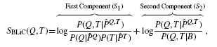
The BLiC score was introduced in Habib et al. (2008) to address the inability of scores like ED to distinguish between a good alignment of informative columns and a good alignment of uninformative columns. BLiC measures the similarity between the ‘query’ column Q and the ‘target’ column T as

(1)

where , and are posterior mean estimates (using a Dirichlet prior or a mixture of Dirichlet priors) of the nucleotide distribution for the query, target and combined columns, respectively, and B refers to the background distribution.

The first component of the BLiC score measures the likelihood that the observed counts of the two columns are generated by a common distribution rather than two distinct distributions and is thus a similarity measure in the spirit of other such scores. The second component penalizes the alignment of uninformative columns as it compares the likelihood that the two columns were generated by a common distribution with the likelihood they were generated by the background distribution. Unfortunately, as we show next, this second component of the BLiC score creates a distinct bias toward motifs composed of a large number of sites.

Let N_Qa be the count of nucleotide a in column Q and let N_Q be the number of sites of the query motif, i.e. N_Q = ∑_a∈N_Qa, where is the four-letter alphabet (similar definitions apply to T). Then, with π_a denoting the background distribution of a∈ we have,

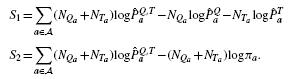In Section 1 of the Supplementary Material, we argue that as N_T→∞, assuming does not converge to the background distribution π, S₂→∞, whereas |S₁| remains bounded. This means that the BLiC score prefers target motifs with large N_T regardless of the query motif. A graphical representation of this phenomenon is presented in Supplementary Figure S1. The following experiment demonstrates that this bias is not just a hypothetical mathematical curiosity.

We implemented the BLiC score in Tomtom and selected the first motif in TRANSFAC to search against all the motifs in the TRANSFAC database (including the query motif). Tomtom reports a list of matches ranked according to the significance of the alignment score. The alignments are schematically presented using motif logos (Schneider and Stephens, 1990). The top three hits in TRANSFAC are shown in Figure 3. For ED, the top hit is, as expected, the query motif itself. However, the top three hits using the BLiC score do not look remotely like the corresponding query motif. As it happens, the top three hits for the BLiC score have a large number of sites associated with them. The analysis above, as well as further examples below, demonstrate that the BLiC score suffers from a significantly compromised retrieval accuracy. This detrimental effect is particularly pronounced when querying a database which has a few deep motifs such as TRANSFAC. Thus, while the BLiC score is effective at reducing the number of uninformative alignments, it is not suitable as a general similarity score. This motivates our following, alternative, approach to reducing spurious uninformative alignments that does not materially compromise the retrieval accuracy.

Fig. 3.

Top three TRANSFAC hits to the query TRANSFAC motif M00001.The figure shows the top three TRANSFAC alignments Tomtom found in response to the query TRANSFAC motif M00001 using BLiC (a) and ED (b) similarity scores. The visual alignments clearly show that using the BLiC score ranked undesirable alignments as top hits, whereas ED assigns the highest ranks to motifs that appear similar. The top three target motifs for the BLiC score have 389, 274 and 235 sites, respectively. These numbers are relatively large when compared with the average number of sites in TRANSFAC (29.5).

3 ALIGNMENT SELECTION

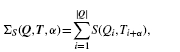
How can we prevent Tomtom from selecting the alignment portrayed in Figure 1C The current prevailing alignment scoring scheme is linear, that is, the alignment is scored as the sum of the similarity scores of the aligned columns. More explicitly, let Σ_S(Q, T, α) denote the similarity score of the ungapped alignment α between the query motif Q and the target motif T using the column similarity score S. Then

(2)

where Q_i, T_i are the columns of Q, T, the alignment α is identified with the offset between Q₁ and T₁, |Q| is the width or length of the query and S is conveniently defined as 0 when i+α∉[1, |T|].

Because the score is linear in the number of aligned columns, it needs to be normalized before we can compare alignments. Tomtom normalizes the alignment score by computing its ‘offset P-value’. The latter is an alignment specific P-value, which is the probability that a random alignment of the same length will have a better score. Random here refers to an iid model for the target motif columns:

where R is a random motif whose columns R_i are drawn with replacement from 𝕋, the reservoir of all target columns (note that we only need to draw the aligned number of columns). After normalizing the alignment scores, Tomtom selects the one with the optimal, i.e. minimal, offset P-value.

While this approach in general yields a very high retrieval accuracy (Gupta et al., 2007), when it comes to filtering uninformative alignments as in Figure 1C, the approach cannot overcome the fact that most scoring schemes give this alignment a maximal score. One way to address this problem is to look at the unaligned part of the motif, a segment which is typically ignored by existing tools, including Tomtom. Specifically, we would like to assign scores to unaligned columns in such a way that unaligned informative columns would contribute less than unaligned uninformative columns. Such a scheme would prefer the alignment in Figure 1D over the one in Figure 1C.

In (2) we used the convention S(Q_i, ∅): = 0 so that only aligned columns get scored. Instead of that, we now propose to define a ‘complete’ version of S, denoted as S_c as follows. S_c agrees with S on aligned columns; however, S_c(Q_i, ∅): = m_i, where m_i is the median of the set {S(Q_i, T) : T∈𝕋}, i.e. m_i is the median score of randomly aligning a target column to Q_i. By assigning the average null score to any unaligned columns, we place all alignments scores on the same scale since all the query columns are considered for each alignment.

Moreover, recall that most column similarity scores such as ED assign the same perfect score to columns with identical composition, regardless of whether they are informative or not. It follows that for a typical target database max{S(U, T) : T∈𝕋} = max{S(A, T) : T∈𝕋}, where U is an uninformative uniform column and A is a maximally informative all-A column. At the same time, these similarity scores also typically satisfy S(A, X) < S(U, X), where X is an all-X column for X∈{C, G, T}, and it follows that min {S(U, T) : T∈𝕋} > min {S(A, T) : T∈𝕋}. This explains why in practice m_i is higher when Q_i = U than when Q_i = A (Table 1 and Supplementary Fig. S6). Therefore, this new approach effectively assigns a lower score to an unaligned informative column than to an unaligned uninformative column, guaranteeing that our modified score will rank the alignment in Figure 1D higher than the one in Figure 1C.

Table 1.

Median scores

	A	C	G	T	U
ED	− 1.046	− 1.080	− 1.080	− 1.046	− 0.548
PCC	0.243	0.194	0.194	0.243	0.674
SW	0.907	0.834	0.834	0.907	1.699
KLS	− 0.967	− 1.040	− 1.040	− 0.967	− 0.269
ALLR	− 1.465	− 1.640	− 1.640	− 1.465	− 0.419

The median null column scores of an all-A, all-C, all-G, all-T and a uniform column. The null distribution was generated using Tomtom by scoring, using the specified column score, the alignment of the corresponding column against every column in TRANSFAC (as well as its reverse complement). The median null score of the uninformative column (U, bold) is higher than that of any of the informative columns. ED stands for Euclidean distance, PCC for Pearson's correlation coefficient (Section 7.2 in Supplementary Material), SW refers to the Sandelin–Wasserman score (Section 7.4 in Supplementary Material), KLS to the symmetric Kullback–Leibler divergence (Section 7.5 in Supplementary Material) and ALLR to the average log-likelihood ratio (Section 7.3 in Supplementary Material).

The discussion above motivated and introduced our new scoring scheme. However, for computational convenience, it is beneficial to introduce the following twist on our last score. Note that is constant for a given query. Hence, if we subtract μ from our newly defined alignment score, we get an equivalent score: the ranking of the alignments of the database motifs to the given query is not affected by a constant shift. This new score is formally quite similar to the standard score in (2) and is therefore significantly easier to incorporate into Tomtom. We refer to it as the ‘complete score’.

(3)

When presented this way, our new score once again ignores unaligned columns. However, note that now the median null score of an aligned query column is 0 so this modified scheme is consistent with our original score motivated above.

Note that the complete score is a transformation of a column similarity score, rather than a score per se, so for example, ‘complete-ED’ stands for (3) with ED for S.

4 SIGNIFICANCE ASSESSMENT

Having normalized the alignment score, we now need to assign an overall statistical significance to the score of the optimal alignment between the given query and target motifs. As mentioned above, Tomtom relies on an iid column model to compute the offset P-values for each alignment. Tomtom then makes the approximating assumption that the scores, and therefore the offset P-values, of different alignments are independent. Under this assumption, the optimal offset P-value is essentially distributed as a minimum of uniformly distributed random variables whose distribution is readily available (Tomtom refers to this overall P-value of the minimal offset P-value as the ‘motif P-value’).

Making the same pair of assumptions, we compute an overall query–target P-value for the optimal alignment score (3) as outlined next. First, mapping the scores to a lattice, we compute the distribution of the latticed null alignment similarity score for each alignment using the same dynamic programming (DP) mechanism that Tomtom uses to compute its offset P-values. Recall that, unlike Tomtom, we select the best alignment based on its (complete) score rather than its offset P-value.² Therefore, at the second step we need to compute the distribution of the maximal of all possible latticed alignment scores. Of course, the different alignment scores are not uniformly distributed; however, adopting the independent alignment assumption that Tomtom is making, we can still find the distribution of this maximum using a straightforward DP approach (see Section 3 in Supplementary Material for discussion of the accuracy of the DP-computed P-values). This method allows us to assign a P-value to the optimal complete alignment score in a process that is not significantly slower than the current one employed by Tomtom.³

Motivated by our goal of reducing uninformative alignments, we also introduce a hidden Markov model (HMM) of a target motif that is more appropriate than the iid model for capturing the tendency of uninformative columns to cluster. The topology of the Markov chain is specified in Figure 4. A key feature of this model is the partition of the columns to ones with high versus low information content (Stormo, 2000). Accordingly, each of the HMM states consistently emits either informative or uninformative columns.

Fig. 4.

Topology of the null target motif HMM. The LL (leading), L and TL (trailing) states emit low information content columns before, within and after the ‘core’, respectively. The H state emits columns with high information content. The I and T state are the silent initial and terminal states, respectively.

The LL and TL states are designed to capture the occasional leading or trailing stretches of uninformative columns. Because the transitions between the states are learned from a reference motif database,⁴ the reference database, from which the distributions of column scores are estimated, is identified with the target database but this can be loosened here. the transitions can capture phenomena such as leading, trailing or internal stretches of uninformative columns (LL/TL/L).

STAMP (Mahony and Benos, 2007) uses a somewhat similar model, originally introduced by Sandelin and Wasserman (2004), to estimate the significance of the match between motifs. There are two notable differences between the latter and our HMM. First, Sandelin and Wasserman only model the first and last columns rather than leading and trailing stretches. Second, their model is an iid mixture model so it cannot model dependencies between columns which are crucial to the modeling of clusters of uninformative columns. See also Piipari et al. (2010) for a related, albeit more complex, approach.

In our analysis, we used a cutoff of 0.5 to determine whether a column has a high or low information content. Using this cutoff, we could unambiguously label each motif in the reference database, i.e. infer the hidden states. Thus, training becomes trivial: we used a simple maximum likelihood estimation for estimating the transition probabilities, while the column emission distributions were set to the observed empirical distributions of each state. In other words, new columns emitted from state X are sampled from the set of reference motif columns that were annotated as emitted from state X.

Once trained, we use our HMM to estimate the significance of an optimal query–target match through a Monte Carlo (MC) sampling scheme. Explicitly, we use the HMM to generate N random motifs of exact length |T| (target motif length), and we find the optimal alignment score for each. This procedure gives us a sample of size N from the null distribution of the optimal query–target match score (conditioned on the given query as well as on the target length). If N is sufficiently large, then the derived empirical distribution can be used to assign a P-value for the observed match score.

Note that while generating a null target motif of a specified length can be done through rejection—reject any path that does not end at state T at step |T|+2—a more efficient sampling can be achieved by conditioning on the last event (0, ). See Section 2 in Supplementary Material for more details.

5 RESULTS

In this section, we compare the performance of various combinations of methods for selecting an optimal query–target alignment with methods for assigning an overall motif P-value. Each such ‘target function’ (alignment-selection and motif P-value evaluation) is assessed with respect to two criteria: reduction of uninformative alignments and retrieval accuracy. We begin with the former criterion.

5.1 Reduction of uninformative alignments

To keep our benchmarks realistic, we chose to study the number of uninformative alignments in the context of a real motif database: the mouse PBM database consisting of 386 motifs (Newburger and Bulyk, 2009). In summary, for each target function we noted the percentage of uninformative alignments among all significant alignments reported when the mouse PBM database was queried against itself.

We define an alignment as uninformative if all the aligned columns of both the query and the target have an information content less than 0.5. An alignment is called significant if its P-value is less than a pre-determined false positive rate (FPR). In Supplementary Figure S4, we compare the performance of several target functions by plotting the percentage of uninformative alignments out of all significant alignments as we vary the significance threshold. Table 2 provides a similar comparison of the ability of several target functions to filter out uninformative alignments only with the significance threshold fixed at the canonical FPR of 0.05.

Table 2.

Reduction of uninformative alignments and retrieval accuracy

Column	Optimal alignment	Overall (motif)	Uninformative alignments	Mean AUC
score	selection	P-value	% at FPR of 0.05
ED	iid offset P-value	ind alignments (TT)	>22.9	0.9994
PCC	iid offset P-value	ind alignments (TT)	>24.9	0.9994
KLS	iid offset P-value	ind alignments (TT)	>22.1	0.9997
SW	iid offset P-value	ind alignments (TT)	>23.3	0.9995
ALLR	iid offset P-value	ind alignments (TT)	>6.2	0.9984
ED	HMM offset P-value	HMM (MC)	>13.7	0.9754
Complete-ED	Motif score	HMM (MC)	< 0.1	0.9869
Complete-ED	Motif score	iid (MC)	< 0.1	0.9791
Complete-ED	Motif score	ind alignments (DP)	< 0.1	0.9994
Complete-PCC	Motif score	ind alignments (DP)	< 0.1	0.9994
Complete-KLS	Motif score	ind alignments (DP)	< 0.1	0.9996
Complete-ALLR	Motif score	ind alignments (DP)	< 0.1	0.9985
Complete-SW	Motif score	ind alignments (DP)	< 0.1	0.9990

Comparison of several target functions (a combination of alignment selection and an overall P-value estimation) in terms of reduction of uninformative alignments and retrieval accuracy. The first column specifies the column similarity method (see Table 1 for the meaning of ED, PCC, KLS, ALLR and SW). All these scores were originally implemented in Tomtom and were modified here to their complete versions (3) where the prefix ‘Complete’ is used. The second column specifies how the optimal alignment is chosen. Tomtom selects the optimal alignment based on the offset P-value computed relative to an iid null model. We also tested computing the offset P-values relative to our HMM (sixth row) and selection based on the maximal complete score (starting from the seventh row). The third column specifies how the overall P-value is computed. Tomtom uses an independent alignments assumption (ind alignments'), ‘MC’ refers to Monte Carlo estimation where the P-value is estimated by generating 10 000 samples for each target motif using either the HMM or the iid null target model. ‘ind alignments (DP)’ refers to our DP calculation of the P-value of the optimal complete score using an independent alignment assumption. The fourth column specifies the percentage of the significant alignments that are uninformative. An alignment is considered significant if its overall P-value computed using the indicated method is below the 0.05 threshold. The alignment is considered uninformative if the information content of all aligned columns is less than 0.5. The fifth column specifies the average of the AUC over all queries. Note that the first row is the current default in Tomtom. All experiments were done using the mouse PBM database. For comparison, using the BLiC score yields the same reduction in uninformative alignments as any of the complete scores but also the worst AUC of 0.9645. While this retrieval accuracy might still be acceptable when the database contains deeper motifs the BLiC AUC drops significantly (see Supplementary Table S2 and Section 2).

The results show that there is a drastic reduction in the percentage of uninformative alignments when the optimal alignment is selected using complete scores, regardless of which column similarity score or overall P-value method is used. This effect is most readily observable in Table 2, where we can see a reduction in uninformative alignments from 22.9% for Tomtom using ED to nearly zero uninformative alignments for any complete score.

How much reduction do we get by replacing Tomtom's iid target null model with the more complex HMM? To gauge that we kept the ED similarity score but used MC sampling from the HMM to estimate the offset, or alignment specific, P-values. Then, selecting the alignment with the optimal P-value we estimated the overall P-value again using MC sampling from the HMM. The result shows that while the HMM generates a substantial reduction in the percentage of uninformative alignments (down from 22.9% to 13.7%), it is far less striking than the reduction obtained by using any of the complete scores.

The performance of the ALLR score merits some discussion as it is significantly more effective at filtering out uninformative alignments (6.2%) than any of the other column similarity scores Tomtom offers. Consistently, ALLR is the only such non-complete column similarity score which can differentiate between perfect alignments of informative and of uninformative columns. Still, when ALLR is compared with any of the complete scores, including a complete-ALLR, the results show that there is room for further reduction in the number of uninformative alignments. This observation is not only a benchmark issue. The same uninformative alignment depicted in Figure 2 comes up as significant when using the ALLR, but is not reported as such if either complete-ED or complete-ALLR are used.

5.2 Retrieval accuracy results

To study the retrieval accuracy of the various combinations that make our target functions, we adopted a framework inspired by the ones used in Habib et al. (2008) and in Gupta et al. (2007). The general idea is to repeatedly sample motifs from the database to create a query database and then quantify, using each of the studied target functions, how many queries are correctly paired with the target motif from which they were sampled.

While the details of our experimental setup are given below, Table 2 summarizes the retrieval accuracy of all the target functions we consider. The table shows that all the methods yield a very high mean AUC (area under the receiver operating characteristic, or ROC, curve), so there is little to choose from in that sense. This observation is consistent with the results reported in Gupta et al. (2007). Having said that, we note that all the methods that use MC sampling to estimate the P-values have a slightly lower mean AUC. This is most evident in the decline of mean AUC when using MC sampling versus the DP computation to estimate the P-values of alignments selected using complete-ED: mean AUC of 0.9791 and 0.9994, respectively (rows 8 and 9). See more on this in Section 6.

The specific experimental design is as follows. We randomly select from the mouse PBM database 80 motifs which will serve as templates for generating randomized queries of the same width w as that of the template motif. Each randomized query is generated by first setting the number of sites, N, to 5, then 10 and then 20. Then, each of the w columns of the template motif PWM is associated with a Dirichlet distribution on ℝ⁴ parameterized by the vector obtained from multiplying the column's frequencies by N. We then sample each column of the randomized query from the corresponding Dirichlet distribution.

We further add variation to these motifs by varying the ‘coverage’ of the sites. Specifically, we either take the full site or remove up to 0.3w columns from a randomly chosen end of the motif. The number of columns to be removed and which end to remove it from are chosen uniformly. Finally, we add additional noise to some of the query motifs by either adding an informative column for motifs with full sites or adding 1 or 3 uninformative columns at an end of a motif that was not previously truncated. This process yields a total of 1680 motifs to query against the target of the mouse PBM database.

For each query motif, we rank the target motifs according to the overall P-value of their match to the query. The query–target pairs that are from the same motif are labeled ‘true’, and those that are not from the same motif are marked ‘false’. A ROC curve plots the fraction of the true positive pairs as a function of the fraction of false positive pairs. The area under this curve (AUC) corresponds to the probability that a score function will rank a randomly chosen positive pair higher than a randomly chosen negative pair. A perfect score function will have an AUC of 1.0, whereas a random score function will have an AUC of 0.5. The AUC is calculated for each query motif against the target database, and the mean AUC (over all queries) is reported in Table 2 for different score functions.

We repeated a similar experiment using the TRANSFAC database (see Section 5 in Supplementary Material). The findings there largely repeat the ones observed in the mouse data: for each of Tomtom's similarity scores, the retrieval accuracy of our complete version combined with the DP-computed P-values is essentially the same as that of Tomtom. At the same time, using MC methods to estimate the P-value slightly compromises the retrieval accuracy.

The experiments above were asymmetric in that mostly the query motifs were randomly missing key motif columns (by truncation). In addition, the query motifs were generated by sampling columns using a Dirichlet distribution. Therefore, to broaden the scope of the tests of our complete scores we designed an additional set of experiments where (i) we generated queries by sampling sites and (ii) to simulate cases where the target motifs miss a growing number of key columns of the motif, but without resorting to truncation which would create artificially short target motifs, we added an increasing number of randomly selected target database columns to the query motifs. The precise protocol and the results are described in Section 6 in Supplementary Material. Qualitatively, we noticed that as the percentage of added query columns was increased from 10% to 100%, the complete scores showed very little loss in retrieval accuracy when compared with the raw scores. More precisely, for the experiments using the mouse PBM and TRANSFAC databases, the loss was negligible throughout the entire range, whereas for experiments based on the MacIsaac yeast database, the loss was negligible when no >50% columns were added to the query and increased after that to ~1% loss in mean AUC when adding up to 100% columns. See Section 6 below for further analysis.

6 DISCUSSION

Habib et al. (2008) offered a possible explanation for the phenomenon of uninformative alignments, wherein a motif database search tool such as Tomtom reports as significant an alignment consisting of uninformative columns. They pointed out that most similarity scores do not distinguish between good alignments of informative and of uninformative columns.

Habib et al. then introduced the BLiC score to address this issue. Our analysis shows that while the BLiC score is effective at reducing the number of uninformative alignments, it can significantly reduce the retrieval accuracy. While one can design post-processing tools to filter out uninformative alignments, we preferred the more principled approach in the spirit of Habib et al. This is not only a question of elegance and deeper understanding of the issues; indeed, post-processing tools tend to compromise the statistical significance analysis in a way that is very difficult to fix. Therefore, we tested a two-pronged approach to reducing the number of uninformative alignments: by modifying the way, we select the optimal query–target alignment, and by testing with respect to a more sophisticated null model.

The evidence presented above indicates that our initially designed two-pronged approach is somewhat of an overkill. Indeed, our general approach to selecting the optimal alignment using complete scores (3) has proven quite effective on its own at removing uninformative alignments for all similarity scores we looked at. At the same time, the new version of Tomtom that uses the complete scores exhibits a retrieval accuracy which is essentially as good as the original method employed by Tomtom (see comment below) with no significant runtime penalty. Taken together, our new recommended settings for Tomtom is to use the new –complete-scores option available in the MEME Suite. More generally, our complete scores can in principle assist any motif database search tool, which uses a linear similarity score (2), to reduce the number of uninformative alignments.

The complete scores exhibit negligible loss or indeed some gain in retrieval accuracy when applied to reasonably well curated databases where the target motifs do not lack more than a third of the motif columns. Even when the database motifs were simulated to be missing up to 50% of the motif columns the complete score's loss of retrieval accuracy was negligible when we used the mouse PBM and TRANSFAC. A similar experiment at this extreme setting but using the MacIsaac yeast database showed a loss of 1% in retrieval accuracy. There are a couple of possible explanations for this difference. First, the yeast database is significantly smaller than the other two: 1218 columns in total versus 6295 (mouse PBM) and 10 642 (TRANSFAC). Because we estimate from the target database the significance as well as the medians that are crucial for the complete scores, a significantly smaller database implies a much larger variability in the results. Second, the median motif length of the yeast database is 9, whereas it is 16 for the mouse PBM data and 12 for TRANSFAC. Again, the smaller motif length could imply more variability when testing for partial matching.

We were puzzled by the slight decline in retrieval accuracy when using the more sophisticated HMM, when compared with the iid model (Table 2). One possible explanation lies in the MC simulations which we use to evaluate the P-value under the null HMM. Indeed, when we increased the number of MC simulations per target motif from 1000 to 10 000 we observed an increase in retrieval accuracy (mean AUC of 0.9785 to mean AUC of 0.9869 under the same experiment described in Section 2 using HMM P-values for complete-ED).

Furthermore, we compared the retrieval accuracy of the complete scores (3) combined with the iid null target model with P-values computed in two different ways: using MC simulations versus using the DP approach described in Section 4. In this case, the DP computed P-values consistently demonstrated better retrieval accuracy than the MC generated P-values (using 10 000 samples). If we can make the leap of faith that a similar principle is at work for the null HMM, then that would again point to the MC sampled P-values as the cause of the inferior retrieval performance of the HMM compared with the iid model.

Finally, on this issue, we suspect that ties, in particular, compromise the power of MC sampled P-values. Using 10 000 samples to evaluate the P-values, we observed a non-negligible number of cases where the selected target motif shared the same P-value with a few other target motifs.⁵ Our analysis showed that, had all these ties been broken in favor of the correct target, then the retrieval accuracy would have been at least as good as Tomtom's.

The HMM described in Figure 4 proved redundant here: its retrieval accuracy was slightly lower when compared with the complete scores or the raw scores, and the MC significance evaluation made it significantly slower as well. As explained in detail above, we believe that we could address both drawbacks by developing a DP algorithm to compute the significance under the HMM null model. However, currently, we are not motivated to design such an algorithm because the complete score achieved our stated goal. We might revisit this issue in the future. For example, in order to effectively apply the complete score one must verify, as in Table 1, that the median null score of an uninformative column is higher than the median of an informative column. While we cannot at the moment imagine a scoring system for which that would not be the case, one could still use the HMM for such a score. Similarly, the experiments with the MacIsaac yeast motif database suggest that when querying against a rather small database that includes many motifs that are missing a significant number of key columns, there is a small price to pay when using the complete scores.

The complete scores defined in (3) assign the median of the null target column similarity score to each unaligned column. This approach is akin to randomly selecting a target column to align to the unaligned query column. We considered quantiles other than the median, and we found that both in terms of reducing uninformative alignments and in terms of retrieval accuracy the method is quite robust to the exact value of the quantile (Section 4 in Supplementary Material).

Finally, the ALLR score is unique among the (incomplete or raw) column similarity scores considered here in the sense that it can differentiate between perfect matches of informative and of uninformative columns. Undoubtedly, this property contributes to the ALLR score being the most effective at filtering out uninformative alignments. Still, as we showed, any complete score (including complete-ALLR) does a significantly better job at removing such alignments. Moreover, our findings and to a larger extent the ones in Gupta et al. (2007) show that ALLR is not optimal as far as retrieval accuracy is concerned.

REFERENCES

- Crooks G, et al. Weblogo: a sequence logo generator. Genome Res. 2004;14:1188–1190. doi: 10.1101/gr.849004. [DOI] [PMC free article] [PubMed] [Google Scholar]
- Das M, Dai HK. A survey of DNA motif finding algorithms. BMC Bioinformatics. 2007;8(Suppl. 7):S21. doi: 10.1186/1471-2105-8-S7-S21. [DOI] [PMC free article] [PubMed] [Google Scholar]
- Durbin R, et al. Biological Sequence Analysis. Cambridge University Press, New York: 1998. [Google Scholar]
- Gupta S, et al. Quantifying similarity between motifs. Genome Biol. 2007;8:R24. doi: 10.1186/gb-2007-8-2-r24. [DOI] [PMC free article] [PubMed] [Google Scholar]
- Habib N, et al. A novel Bayesian DNA motif comparison method for clustering and retrieval. PLoS Comput. Biol. 2008;4:e1000010. doi: 10.1371/journal.pcbi.1000010. [DOI] [PMC free article] [PubMed] [Google Scholar]
- MacIsaac KD, et al. An improved map of conserved regulatory sites for Saccharomyces cerevisiae. BMC Bioinformatics. 2006;7:113. doi: 10.1186/1471-2105-7-113. [DOI] [PMC free article] [PubMed] [Google Scholar]
- Mahony S, Benos PV. STAMP: a web tool for exploring DNA-binding motif similarities. Nucleic Acids Res. 2007;35:W253–W258. doi: 10.1093/nar/gkm272. [DOI] [PMC free article] [PubMed] [Google Scholar]
- Newburger DE, Bulyk ML. UniPROBE : an online database of protein binding microarray data on protein – DNA interactions. Nucleic Acids Res. 2009;37(Suppl. 1):D77–D82. doi: 10.1093/nar/gkn660. [DOI] [PMC free article] [PubMed] [Google Scholar]
- Piipari M, et al. Metamotifs–a generative model for building families of nucleotide position weight matrices. BMC Bioinformatics. 2010;11:348. doi: 10.1186/1471-2105-11-348. [DOI] [PMC free article] [PubMed] [Google Scholar]
- Portales-Casamar E, et al. JASPAR 2010: the greatly expanded open-access database of transcription factor binding profiles. Nucleic Acids Res. 2010;38(Suppl. 1):D105–D110. doi: 10.1093/nar/gkp950. [DOI] [PMC free article] [PubMed] [Google Scholar]
- Sandelin A, Wasserman WW. Constrained binding site diversity within families of transcription factors enhances pattern discovery bioinformatics. J. Mol. Biol. 2004;338:207–215. doi: 10.1016/j.jmb.2004.02.048. [DOI] [PubMed] [Google Scholar]
- Schneider TD, Stephens RM. Sequence logos: a new way to display consensus sequences. Nucleic Acids Res. 1990;18:6097–6100. doi: 10.1093/nar/18.20.6097. [DOI] [PMC free article] [PubMed] [Google Scholar]
- Stormo G. DNA binding sites: representation and discovery. Bioinformatics. 2000;16:16–23. doi: 10.1093/bioinformatics/16.1.16. [DOI] [PubMed] [Google Scholar]
- Tompa M, et al. Assessing computational tools for the discovery of transcription factor binding sites. Nat. Biotechnol. 2005;23:137–144. doi: 10.1038/nbt1053. [DOI] [PubMed] [Google Scholar]
- Wingender E, et al. TRANSFAC: an integrated system for gene expression regulation. Nucleic Acids Res. 2000;28:316–319. doi: 10.1093/nar/28.1.316. [DOI] [PMC free article] [PubMed] [Google Scholar]
- Xing EP, Karp RM. Motifprototyper: a Bayesian profile model for motif families. Proc. Natl Acad. Sci. USA. 2004;101:10523–10528. doi: 10.1073/pnas.0403564101. [DOI] [PMC free article] [PubMed] [Google Scholar]
Associated Data
This section collects any data citations, data availability statements, or supplementary materials included in this article.