Combination of Markov State Models and Kinetic Networks for the Analysis of Molecular Dynamics Simulations of Peptide Folding

Abstract

Atomistic molecular dynamics simulations of the TZ1 beta-hairpin peptide have been carried out using an implicit model for the solvent. The trajectories have been analyzed using a Markov state model defined on the projections along two significant observables and a kinetic network approach. The Markov state model allowed for an unbiased identification of the metastable states of the system, and provided the basis for commitment probability calculations performed on the kinetic network. The kinetic network analysis served to extract the main transition state for folding of the peptide and to validate the results from the Markov state analysis. The combination of the two techniques allowed for a consistent and concise characterization of the dynamics of the peptide. The slowest relaxation process identified is the exchange between variably folded and denatured species, and the second slowest process is the exchange between two different subsets of the denatured state which could not be otherwise identified by simple inspection of the projected trajectory. The third slowest process is the exchange between a fully native and a partially folded intermediate state characterized by a native turn with a proximal backbone H-bond, and frayed side-chain packing and termini. The transition state for the main folding reaction is similar to the intermediate state, although a more native like side-chain packing is observed.

Introduction

The energy landscape theory of protein folding(1) asserts that proteins evolved to minimize frustration during the folding process.(2) This suggested that the energy landscape of proteins is globally funneled toward the native state, so that many routes are available for the folding polypeptide chain to reach the native conformation. Thus, the folding process involves the formation of ensembles of increasingly ordered structures as it proceeds down the funnel.^1,3,4 Characterization of the main conformers of the protein and the ways taken to move from one to the other is a fundamental objective of protein folding research.

While experiments provide the primary evidence regarding protein folding and its determinants, molecular dynamics (MD) simulations can potentially add up important information thanks to the atomistic resolution they provide.(5) Ideally, if the force field used were accurate enough and if computational time was sufficient, MD simulations could directly identify all the protein conformers and transitions between them. Even in that case, however, we would be challenged by the enormous amount of data which constitute the MD trajectory. How can we extract the relevant information from the trajectory and provide it in a “human readable” form without losing or overlooking any important details?

A tractable representation of the dynamics of the protein corresponds to providing, e.g., populations of conformers and their rates of exchange. A large variety of methods have been proposed to address this point. On one hand, there are approaches based on the projection of the dynamics along a series of observables (i.e., the end-to-end distance, the radius of gyration, root mean squared deviation (rmsd) from reference structure, dihedral angles, etc.). Such methods have the advantage of providing the results with a clear and immediate meaning, but may lead to missing the relevant degrees of freedom, as we project an intrinsically multidimensional system onto the few dimensions represented by the observables.^6,7 On the other hand, another class of approaches is based on a discretization of the trajectory via clustering, where conformations of the peptide chain are grouped together when they are similar according to some metrics defined directly in the multidimensional space of the peptide chain. These approaches reduce the risk of missing relevant degrees of freedom and allow for the determination of purely kinetic properties such as commitment probabilities and mean first passage times.⁸⁻¹² However, they usually require further complex steps of analysis like Markov state models^13,14 or procedures to recover the free energy basins^12,15 to reach an accurate and concise description of the system.

Markov state models (MSM) have received increasing attention as a powerful tool to analyze and integrate MD trajectories and obtain a concise and unbiased view of the dynamics of biopolymers.^{13,14,16−21} On the basis of the assumption that on a long enough time scale the biopolymer dynamics can be represented as a Markov process, these procedures naturally provide a way to identify the relevant macrostates of the system and their exchange rates. The procedures usually require an initial discretization of the trajectory into microstates that have to satisfy certain criteria; e.g., conformations separated by free energy barriers have to belong to different microstates,(13) and the size of the microstates has to be sufficient to provide a statistically significant estimate of the transition probabilities into the other microstates. These requirements cannot always be enforced from the beginning of the analysis. Although MSMs provide tools to check a posteriori the Markovianity of the system, other ways to cross-check the results and identify possible weaknesses in the model can improve the overall description and understanding of the biopolymer dynamics.

Here, we analyze extensive MD simulations of a model β-hairpin, for which hundreds of folding and unfolding events could be sampled, thanks to the adoption of a continuous model for the solvent. Using a Bayesian approach,^18,19 we optimize a MSM to fit the trajectories projected onto two relevant observables, and from the eigenvectors of the rate matrices we extract information on the macrostates involved in the slowest relaxation dynamics. Then, we evaluate the Markovianity of the description. Beside the Markov state analysis, we carry out a kinetic network analysis^9,22 which consists of building a network (or graph) out of the clustered trajectories by associating the conformational clusters with the nodes of the network and the observed transitions with the links between nodes. We then merge the results of the Markov state analysis and those of the kinetic network analysis. This is done by projecting the Markov macrostates on the network representation and using the Markov macrostates as target states for folding commitment probability calculations on the network. We show that this combined approach allows for the determination of the main conformers of the peptide, their exchange rates, and also the transition state ensemble, and helps to provide a concise view of the peptide dynamics. The methods described are found to be particularly useful in the present case, as they allow for the identification of different conformers within the denatured state ensemble. This is especially important because partially unfolded and denatured states of proteins have been implicated in several cellular processes, and the importance in cellular function of natively unfolded and marginally stable proteins is being increasingly recognized.(23) Similarly, the role played by the residual structure of the denatured states in determining the folding process needs to be carefully evaluated.(24) We finally provide a structural and thermodynamic description of the states identified for the hairpin peptide.

Methods

Simulation Protocols

The 12-residue β-hairpin tryptophan zipper 1 (TZ1, Figure 1, pdb ID 1LE0)(25) with a type II′ turn and a core of four interlocking tryptophan residues was modeled using implicit-solvent molecular dynamics simulations. Simulations were run using the program CHARMM,(26) with all heavy atoms and polar hydrogen atoms being modeled explicitly using a united-atom parametrization (PARAM19). The aqueous effects of the solvent on the solute are described by a mean-field approximation based on the solvent-accessible surface area (SASA) of the peptide.(27) To improve sampling, solute–solvent frictional forces have been neglected; this has no appreciable effect on the thermodynamic properties of the system. Initial atomic positions are extracted from the NMR structure.

Figure 1.

The 12-residue β-hairpin TZ1: from the Protein Data Bank with (a) backbone carbon (cyan), nitrogen (blue), oxygen (red), and hydrogen (white) atoms and residue labels, and (b) tryptophan side-chains and secondary structure, with gray for random coil, red for extended β-sheet, and tan for turn sequence.

Ten MD simulation trajectories of 2 μs each and different initial velocities were run at 300, 330, and 360 K. The temperature was kept constant during the simulations by weak coupling to an external bath, as described by Berendsen et al.,(28) with no pressure constraints being imposed on the system. The SHAKE algorithm(29) was used to fix covalent bond lengths, allowing a 2 fs integration time step.

Structural Analysis

The trajectories were examined by observing the deviation from the NMR structure in the root-mean-square distance (rmsd) between backbone C_α atoms. The number of backbone hydrogen bonds (H-bond) was also examined for the peptide. Instead of using a step function to describe a H-bond as either formed (1) with an interatomic distance of less than 2.6 Å or not formed (0) with an interatomic distance in excess of this cutoff, a sigmoidal function of the distance d was used f_HB(d) = 1/(1 + (x/2.6)⁶). Using this method, a continuous range of values between 1 and 0 is obtained, with f_HB(d = 2.6 Å) = 0.5 representing a conformation with an interatomic distance of exactly 2.6 Å, f_HB(d) values close to 1 representing conformations with interatomic distances less than 2.6 Å, and values close to 0 representing conformations with interatomic distances greater than 2.6 Å.

Five native H-bond contacts were identified along the backbone of the native conformation. Since the H-bond nearest to the turn sequence was formed for conformations in all states, the remaining four H-bonds were taken as a reference by which to assess the degree of nativeness of a given structure, through the variable HB = ∑_if_HB(d_i), where the sum is extended to the four H-bonds.

Definition of the Microstates for the Markov State Model

The globally funneled energy landscape theorized for protein folding allows for a significant reduction in the complexity of the description provided that simple reaction coordinates are found to capture the folding process.(1) In this study, the simulation trajectories were projected along the observables HB and rmsd and binned into N two-dimensional microstates. Thus, each bin/microstate is defined by both a range of HB values and a range of rmsd values. In this way, a discretized trajectory s(t) ∈ [1,2,...N]∀t ∈ [0,T_f] was obtained, where T_f is the total simulation time. Uniform binning (i.e., all bins having the same width along each of the two observables) resulted in poor statistics for some of the transitions between microstates, which compromised the accuracy of the rate matrix diagonalization (data not shown). Thus, a variable binning strategy was adopted, which requires a few iterations of the following algorithm. Starting from a single two-dimensional bin containing all the data points, bins containing more than n_tb = 12 000 points were evenly split into four smaller identical bins with halved width along each dimension, and the data points were redistributed in the four smaller bins. No splitting was performed for bins whose width was equal or smaller than (ΔHB = 0.25 × Δrmsd = 0.625), both to limit the total number of bins and to prevent artificial splitting of very similar conformations. This procedure favors a more uniform distribution of the data points into the bins (i.e., the microstates), and eventually leads to more accurate estimates for transition probabilities between microstates. The binning procedure was applied separately for the simulations at 300, 330, and 360 K, resulting in different numbers of bins/microstates at each temperature. The observed probability P_i of each microstate is given by

where t is the time and δ is the Kronecker delta function. The number of transitions observed from microstate i to microstate jN_ji after a lag time Δt is thus expressed as

Markov State Model

Below, the MSM is derived following the formalism proposed by Hummer and co-workers.(18) Assuming that, after the initial lag time Δt, the dynamics observed along the simulation trajectories is Markovian, the probability P_i satisfies a master equation:

where the vector P(t) represents the probability for each microstate at time t and R is a transition rate matrix with constant elements R_ij ≥ 0 for i ≠ j, R_ii ≤ 0, and ∑_iR_ij = 0.

Equation 3 has the solution

If the system converges to an equilibrium distribution, the equilibrium probability P^eq is a right-eigenvector of R with zero eigenvalue, and the system must satisfy detailed balance so that

The matrix exponential of eq 4 can be calculated through the diagonalization of the symmetric matrix R̃:

where P^±1/2 is the diagonal matrix with elements (P_i^eq)^±1/2.

For the diagonalization, the orthogonal matrix U of eigenvectors of R̃ must satisfy the relation R̃U = UΛ, where Λ is the diagonal matrix with eigenvalues of −λ_i. Since UU^T = U^TU, where U^T is the transpose of U, eqs 4 and 6 can be combined:

The left and right eigenvectors of R can be obtained from the eigenvectors of R̃ (note that they have the same eigenvalues):

In addition to the stationary solution P^eq with zero eigenvalue, the other right-eigenvectors of R have negative eigenvalues representing decay rates, and the vectors’ elements sum up to zero. So a system in state i at time t = t₀ has a probability p(j, t₀ + Δt|i, t₀) of being in state j at time t₀ + Δt given by

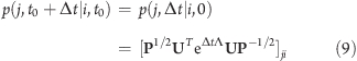The rate matrix R was estimated using Bayesian inference^18,19,30 by constructing a posterior distribution of the model parameters from the simulation data. If a uniform prior distribution of the model parameters is assumed, the posterior distribution is proportional to a likelihood function L, which gives the probability of observing the same motions on the HB-rmsd reaction coordinates in the Markov model as those seen in the simulations:

This may be rewritten in the form

A Monte Carlo sampling of the values of R and P^eq compatible with the simulation data was obtained using −ln(L) as the energy function and by constructing the initial rate matrix R from the equilibrium probabilities P_i (eq 1) and the observed transitions N_ij (eq 2) after symmetrization and normalization. A simulated annealing strategy was used where the Monte Carlo temperature, initialized at 10, was gradually lowered to 1 following an exponential decay as a function of Monte Carlo steps. Only the data obtained with Monte Carlo temperatures below 1.005 were retained for the sampling. The Monte Carlo step size was dynamically adapted in order to obtain an acceptance ratio between 10 and 30%. A total of 10⁷ Monte Carlo steps were performed, and samples of R and P^eq values were saved every 1000 steps. Each sampled R and P^eq pair was individually used to compute the eigenvalues and eigenvectors of the associated Markov model. Eigenvalues and eigenvectors of R were averaged over the sampled data.

On the basis of Perron clustering theory,(31) the microstates were then partitioned into macrostates using information from the slowest non-null left eigenvectors of R. Because of the gap between the third and fourth non-null eigenvalues, we considered the three slowest eigenvectors for partitioning. Each macrostate is defined as the set of microstates having the same signs of the components of the three slowest left eigenvectors used for partitioning. We note that numerically more robust versions of this algorithm have also been presented.^14,32

Cluster Analysis

The Leader algorithm(33) was used to group structures whose distance root-mean-square deviation between C_α and C_β atoms was less than 0.8 Å. This value for the clustering cutoff was chosen as a compromise between smaller values, yielding many small clusters and poor intercluster statistics, and larger values, resulting in heterogeneous structures being grouped in the same cluster. The clustering and other structural analyses were performed using the program WORDOM.(34)

Commitment Probability

The commitment probability p_commit^α,β for a protein conformation is the probability that it will fold into a given state α before reaching state β. There are several methods to measure the p_commit of a conformation.(35) One method is to start a large number of short MD simulations from the given conformation, and record the number of trajectories that commit to a given state of the molecule.(36) The number of trial simulations required for a reliable evaluation of p_commit for the many conformations saved along a trajectory makes this method unfeasible. An alternative method estimates commitment probabilities for all structures in an equilibrium folding/unfolding trajectory without the need for any additional simulations.^10,11 This method is outlined in more detail below.

The probability p_commit^α,β of a single structure i reaching either of the states α or β is given by

where n_α is the number of MD simulations starting from structure i which reach state α and n_tot is the total number of committed MD simulations starting from i.

Since structurally similar conformations have similar kinetic behavior, they also have similar p_commit^α,β.(11) Structures along a trajectory were grouped in structurally similar clusters, as described above, and the segment of MD trajectory following each structure was checked for reaching either the states α or β. The p_commit of a cluster C is defined as the ratio between structures folding into state α and the total number of committed structures in the cluster. Each structure in the cluster is then assigned the p_commit^α,β of the cluster. Although the MSM identified several slow relaxation processes in TZ1, we are mostly interested in the one between the folded and the denatured region of the peptide, i.e., the main folding transition, which, in the present case, is represented by the slowest non-null eigenmode of the rate matrix. Thus, we considered only the sign structure of the slowest non-null eigenvector and we selected the three most populated microstates with a positive eigenvector component (i.e., belonging to the folded region) and the most populated microstate with a negative eigenvector component (i.e., belonging to the denatured region, the denatured region has a much larger population than the native region so a single microstate is sufficient) and used them as targets α and β for measuring p_commit. The α and β subsets are meant to represent the bottom of the free energy well of the native and denatured region, respectively.

The ability of the approximate commitment probability as a reaction coordinate to locate the dominant transition between the folded and denatured states can be evaluated by examining the conformations on a transition pathway. Following Hummer,(37) a transition pathway (TP) is defined as any section of a trajectory leaving a state A and proceeding directly to state B (i.e., without crossing back into A), and vice versa. In our calculations, A and B are the conformations with p_commit ≤ 0.2 and p_commit ≥ 0.8, respectively. A minimum path length of 0.08 ns was imposed to rule out rapid fluctuations at the boundaries of the TPs. The conditional probability that a conformation with a given value of the p_commit coordinate will be on a TP, p(TP_A↔B|p_commit), is then measured directly from the trajectory, and its distribution is compared with the limiting case of the pure unidimensional diffusion to ascertain the quality of our approximate p_commit as a reaction variable for the folding transition.

Kinetic Network Analysis

The conformation space of the peptide, as sampled by molecular dynamics, can be mapped to a network describing the significant free energy minima and their dynamic connectivity, without requiring arbitrarily chosen reaction coordinates. Some studies(6) have found poorly chosen reaction coordinates can mask important details, such as heterogeneity of denatured or transition states, especially in the case of potentials based on physiochemical principles, like CHARMM.

In this case, the “nodes” of the network are the clusters defined previously by the cluster analysis, with direct transitions between clusters along the trajectory representing the “edges” of the network.(9) Two clusters are connected by an undirected link if either they include a pair of structures that are visited within 20 ps or they include structures that are separated by one or more conformations belonging to clusters with less than 20 structures each.

The nodes of the network were ordered on the graph so that close nodes correspond to clusters with a similar link pattern, and colored according to the Markov macrostates defined above.

Results

Identification of Stable States

The stable states of the peptide were identified by optimizing a MSM using Bayesian analysis, as described in “Methods”. Initial calculations carried out using only the backbone H-bonds for the definition of the microstates did not show Markovianity, as reported by the eigenvalue spectrum which did not converge at any lag time (data not shown). Simulations were then projected along both HB and rmsd, and the data were binned into a discrete number of two-dimensional microstates defined by both a range of HB and rmsd values (Figure 2a). Thus, 55, 53, and 41 microstates were obtained at 300, 330, and 360 K, respectively. The variable width of the microstates/bins, obtained using the adaptive binning procedure described in the “Methods” section, reduces the presence of scarcely populated bins which would introduce large uncertainties on the elements of the transition matrix. The MSM was then built using those microstates. The ensemble of rate matrices compatible with the simulation data was obtained using the Bayesian analysis and the likelihood function L (eq 11). The rate matrices were then diagonalized. At all three temperatures (300, 330, 360 K), the slowest non-null eigenvalue converged for lag times not less than 2.56 ns, and a well-defined gap was observed between the slowest and second-slowest non-null eigenvalues (the eigenvector corresponding to the null eigenvalue is the equilibrium state) and between the third and fourth non-null eigenvalues (Figure 2b). The relaxation times for the three slowest processes at the three temperatures are reported in Table 1. Although the slowest relaxation process at 360 K is on average slightly faster than the lag time, the subsequent analysis of the corresponding macrostates provided results in line with those obtained at the lower temperatures, so we decided to present the 360 K data as well.

Figure 2.

(a) Equilibrium distribution of the microstates of the Markov state model fitting simulation data at 300 K (left), 330 K (middle), and 360 K (right). The simulation data binned into the microstates provide very similar (undistinguishable) distributions. The variable width of the microstates in the HB/rmsd space is obtained via an adaptive binning algorithm (see “Methods”) to limit the presence of poorly populated microstates. (b) Relaxation times (inverse eigenvalues) of the Markov state model as a function of lag time for the simulations at 330 K (error bars at 99% confidence interval). Convergence is reached for lag times equal or larger than 2.5 ns. Similar plots are obtained at 300 and 360 K (not shown). First (left), second (middle), and third (right) average non-null left eigenvectors of the rate matrices at (c) 300 K, (d) 330 K, and (e) 360 K. The color scale ranges from black for the smallest (most negative) components to white for the largest (most positive) components, with the midpoint of the scale fixed at 50% gray for the zero components.

Table 1. Relaxation Times of the Markov State Model from the Average Eigenvalues of the Rate Matrices.

	relaxation time (ns)
temperature (K)	1/λ1	1/λ2	1/λ3
300	20.0 ± 0.6	4.6 ± 0.4	4.2 ± 0.1
330	6.7 ± 0.5	2.6 ± 0.2	1.8 ± 0.1
360	2.0 ± 0.1	1.4 ± 0.1	0.8 ± 0.1

The sign of the components of an eigenvector of the rate matrix (note that components of left and right eigenvectors of R have the same sign) tells us which microstates exchange population during the corresponding relaxation process (e.g., the microstates with positive components of the eigenvector lose population in favor of those with negative components, or vice versa, depending on the initial conditions). On the basis of this idea, which has been rigorously formalized in Perron clustering theory,(31) the signs of the components of the first three non-null left eigenvectors of the rate matrices, which give information on the slowest, second-slowest, and third-slowest relaxation processes, respectively, were used to identify four significantly populated stable macrostates, as detailed in “Methods”. Nonsignificantly populated macrostates were lumped into the other macrostates according to structural similarity.

Inspection of the elements of the first eigenvector reveals that it describes the relaxation process between the folded and denatured regions of the peptide’s conformational space. At 300 K (Figure 2c, left), the folded region is roughly defined by a maximum rmsd of 6 Å and between 0.5 and 4 formed HB contacts, and the denatured region is defined by a maximum of 0.25 formed HB contacts for 2.25 Å < rmsd < 6.25 Å and a maximum of 1 formed HB contact for rmsd's above 6.25 Å. The second eigenvector yields more detailed information about the denatured region, which at 300 K (Figure 2c, center) is comprised of two distinct macrostates occupying separate regions on the HB-rmsd projection: the first macrostate is roughly defined by HB < 0.25 and 2.25 Å < rmsd < 3.75 Å and will be referred to as state D1. The second macrostate is roughly defined by HB < 1 and rmsd > 3.75 Å and will be referred to as state D2 (at 360 K, in Figure 2e, middle, there is some scatter with a microstate from D1(dark) in the D2 region; however, this microstate has an extremely low population as reported by Figure 2a, right, and its presence does not affect the validity of our statement). The third eigenvector identifies two subsets of the folded region. The most native-like subset will be referred to as the native state N and will comprise roughly conformations with HB > 0.5 and rmsd < 2.25 Å. The intermediate region (at 300 K with roughly 0.25 < HB < 2 and 2.25 Å < rmsd < 6.25 Å, Figure 2c, right) will be referred to as state I. The eigenvectors at 330 and 360 K show a very similar picture, as illustrated in Figure 2d and e.

In Figure 3, information from all three eigenvectors is merged to yield a picture comprising four stable macrostates at all three temperatures: N (magenta), I (yellow), D1 (blue), and D2 (green).

Figure 3.

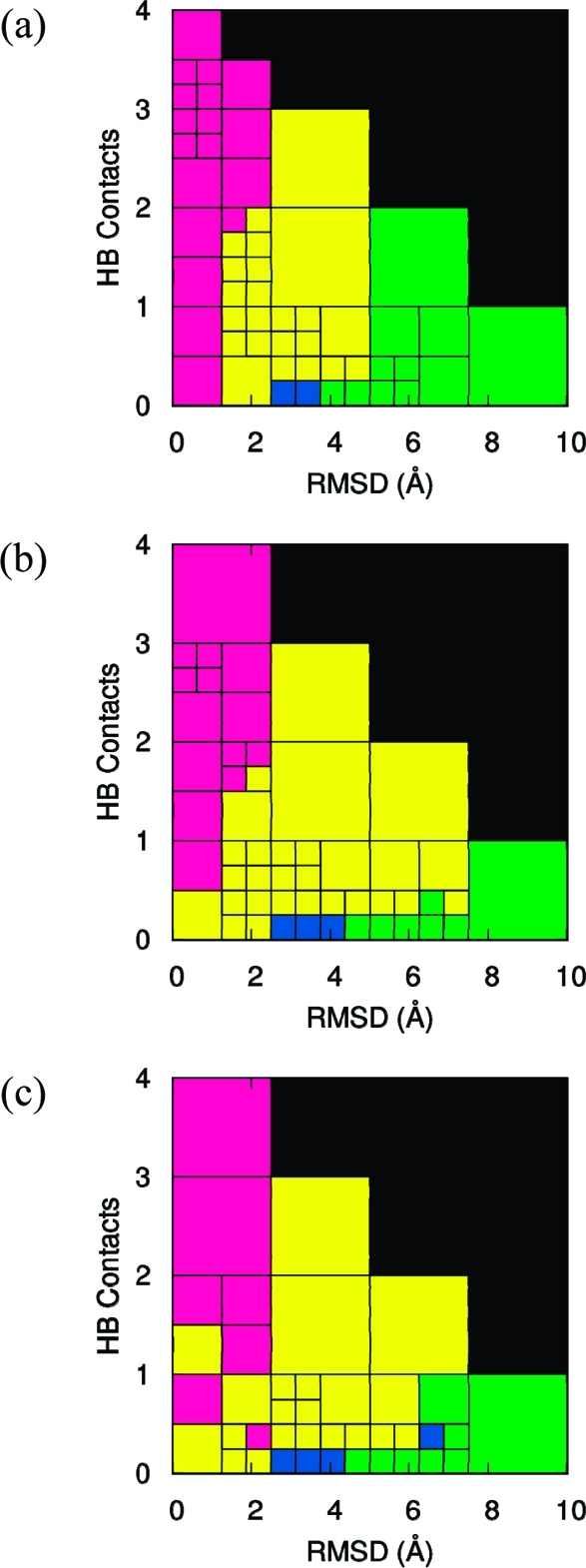
Markov macrostates at (a) 300 K, (b) 330 K, and (c) 360 K obtained by grouping together microstates with the same signs of the components of the three slowest eigenvectors of the MSM. The native state N is shown in magenta, the intermediate state I in yellow, the denatured state D1 in dark blue, and the denatured state D2 in green.

Kinetic Networks

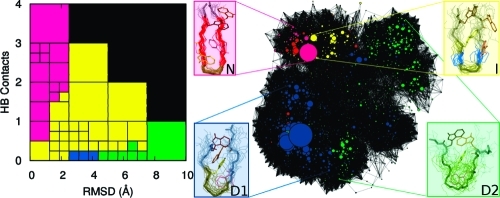
As described in “Methods”, a kinetic network is produced based on the clustering of the MD trajectory. Conformational clusters correspond to the nodes of the network, and the observed transitions correspond to the links between nodes. This mapping allows for the definition of a vector for each cluster whose components are the network distances (i.e., the minimal number of separating links) between the cluster and a set of reference clusters (e.g., the most populated ones). The network can be projected onto a two-dimensional graph, using the first two principal components of the covariance matrix of the cluster vectors.(38) This representation has the advantage of preserving the kinetic similarities between clusters. Thus, the network could be represented in a plot where the clusters were colored according to their most populated state, identified by the MSM analysis, with the same color scheme as in Figure 3. The network analysis performed on the simulations of TZ1 at each temperature (see Figure 4) show the N and I states occupying a small, localized region of the network while the denatured states D1 and D2 occupy the majority of the network. At all three temperatures, the mapping of the macrostates from the MSM analysis onto the kinetic network shows that the Markov states are kinetically partitioned, i.e., different states occupy different regions of the network, with limited overlap.

Figure 4.

Kinetic networks describing the conformation space of the TZ1 peptide at (a) 300 K, (b) 330 K, and (c) 360 K. The nodes of the network are colored according to their most populated macrostate, with the N state being magenta, the I state being yellow, the D2 state being green, and the D1 state being blue. The dominant conformation belonging to each state is also shown. The network pictures are obtained using the program VISONE.(38)

The localization of the N state is particularly prominent at 300 K, where the relative depth of the free energy minima is larger with respect to temperature, as reported by the low link density region separating the native clusters from the rest of the network in Figure 4a. This confirms the presence of free energy barriers between the Markov macrostates, and that the observed denatured states are in a different free energy basin than the folded states. In agreement with the kinetic measurements, the presence of the gap is less well-defined at 330 and 360 K, corresponding to a smaller free energy barrier relative to k_BT, separating N from I. We note that the increase in link density between separate free energy basins as the temperature increases is equivalent to an increase in the available pathways used by the system to connect the basins, in analogy to the findings for the Trp-cage mini protein.(39) At all three temperatures, there is also evidence of a free energy barrier between the D1 state and the most populated region of the D2 state (green), although regions where the two states are mixed are also present on the network.

Commitment Probability

The MSM identified a series of relaxation processes. Each relaxation process can be associated with the crossing of a free energy barrier defined on the free energy landscape of the peptide. The highest barrier, corresponding to the slowest relaxation process, separates variably folded microstates from denatured microstates. The folded microstates, which share the same sign of the first eigenvector components (light-colored microstates in Figure 2c–e, left), comprise both microstates in N and I. The denatured microstates (sharing the opposite sign to the folded microstates for the elements of the first eigenvector, dark microstates in Figure 2c–e, left) comprise both D1 and D2. Smaller free energy barriers split the folded microstates in I and N and the denatured microstates in D1 and D2. Disregarding the smaller free energy barriers, we specifically looked for the main folding transition state associated with the highest free energy barrier. Approximate commitment probabilities for the main folding transition were measured for all the structures collected along the trajectories at each temperature, using the most populated microstates P_i in the folded and denatured regions (as determined by the sign of the first non-null eigenvector) as target states (see “Methods”).

The distribution of commitment probabilities (Figure 5a) shows two distinct peaks at p_commit ≈ 0.0 and p_commit ≈ 1.0, which correspond to the denatured and folded states, respectively (the distribution of p_commit for intermediate values is noisy due to the relatively low number of conformations populating this region). The approximate procedure used to measure the commitment probability, which depends on the clustering algorithm and sampling, may in principle compromise its reliability as a reaction coordinate. Hummer and collaborators^37,40,41 proposed a method to evaluate the quality of a reaction variable r by measuring the conditional probability, p(TP|r), that a conformation will be on a transition pathway (TP) for a given value of r. He showed(37) that, in the limit of diffusive dynamics along r, the transition path probability p(TP|r) is related to the exact commitment probability ϕ(r) by p(TP|r) = 2ϕ(r)(1 – ϕ(r)). Thus, p(TP|r) in the limiting case of a pure diffusive system has a maximum of 0.5 at the transition state, i.e., for ϕ(r) = 0.5. This finding has been used to assess the quality of reaction variables for describing the dynamics of a generic system. In those studies,^40,41 the authors compared the p(TP|r) obtained using several reaction variables. Those variables which provided p(TP|r) distributions close to the diffusive limit (i.e., peak close to 0.5, bell shaped distribution around the peak) are considered good, as they can separate stable and reactive species. Vice versa, those variables giving rise to broad p(TP|r) distributions with a small peak (<0.3) cannot be used to tell unequivocally if a structure is reactive (i.e., if it belongs to the transition state); thus, they do not act as good reaction coordinates. In the present case, the distribution of p(TP|p_commit), shown in Figure 5b, is bell-shaped with a maximum of 0.48 at 300 K, 0.49 at 330 K, and 0.48 at 360 K centered on the region 0.4 ≤ p_commit ≤ 0.55, almost reaching the ideal limit of 0.5 observed in the case of pure unidimensional diffusion. This demonstrates that the approximate p_commit reported in the present work represents a good reaction coordinate.

Figure 5.

(a) Distribution of approximate commitment probabilities shown at 300 K (solid line), 330 K (dashed line), and 360 K (dash-dotted line). (b) The conditional probability of being on a transition pathway for a given value of the approximate commitment probability is shown at 300 K (solid line), 330 K (dashed line), and 360 K (dash-dotted line).

Structural and Thermodynamic Analyses of Macrostates

Once the metastable macrostates and transition state were identified by the Bayesian and commitment probability analyses of the Markov model, respectively, their structural and thermodynamic properties could be examined.

The populations of states D1, D2, I, N, and T were used to calculate their relative stabilities (Table 2):

where P(A) and P(B) are the populations of the two states, N_A is the Avogadro constant, and k_B is the Boltzmann constant.

Table 2. Relative Stabilities of the D1, D2, I, and N States at the Three Simulation Temperatures.

	relative stability ΔGstate1–state2 (kcal/mol)
temperature (K)	D1–D2	D1–N	D2–N	D1–I	D2–I	I–N
300	0.163	1.146	0.982	0.937	0.774	0.208
330	0.382	1.482	1.100	1.143	0.761	0.339
360	0.454	1.750	1.296	1.343	0.890	0.406

The average internal potential energy of each macrostate ⟨E_pot⟩ was calculated from the internal potential energies recorded for each structure along a trajectory (Table 3). The relative enthalpies of the denatured and native state were also compared:

where ΔH(T)_U–N is the enthalpy change at temperature T and ⟨E_pot(U)⟩ and ⟨E_pot(N)⟩ are the average internal potential energies of the denatured (D1 + D2) and native (N) state, respectively. The average number of backbone H-bonds and average rmsd's for each state are shown in Tables 4 and 5.

Table 3. Average Internal Potential Energies of the D1, D2, I, N, and T States Given at 300, 330, and 360 K.

	⟨Epot⟩ (kcal/mol)
temperature (K)	N	I	T	D1	D2
300	29.1 ± 3.5	32.6 ± 3.6	32.9 ± 3.5	33.2 ± 3.5	33.3 ± 3.8
330	44.3 ± 3.8	48.3 ± 3.9	49.3 ± 4.0	48.6 ± 3.9	49.5 ± 4.1
360	60.6 ± 4.2	63.8 ± 4.1	65.4 ± 4.2	64.0 ± 4.2	65.6 ± 4.3

Table 4. Average Numbers of Backbone H-Bonds Given for States D1, D2, I, N, and T at 300, 330, and 360 K.

	HB
temperature (K)	N	I	T	D1	D2
300	2.80 ± 0.20	0.90 ± 0.25	0.88 ± 0.20	0.006 ± 0.009	0.007 ± 0.013
330	2.58 ± 0.26	0.78 ± 0.22	0.61 ± 0.22	0.007 ± 0.011	0.005 ± 0.007
360	1.94 ± 0.40	0.62 ± 0.19	0.44 ± 0.22	0.008 ± 0.012	0.005 ± 0.009

Table 5. Average rmsd's Given for States D1, D2, I, N, and T at 300, 330, and 360 K.

	rmsd (Å)
temperature (K)	N	I	T	D1	D2
300	1.16 ± 0.19	3.05 ± 0.36	2.46 ± 0.23	4.07 ± 0.15	5.15 ± 0.29
330	1.32 ± 0.22	3.17 ± 0.41	3.28 ± 0.31	4.25 ± 0.20	5.50 ± 0.28
360	1.79 ± 0.31	3.43 ± 0.39	3.57 ± 0.44	4.27 ± 0.21	5.66 ± 0.30

As shown in Table 3, the N state has the lowest average potential energy and the denatured states D1 and D2 have the highest average potential energies at 300, 330, and 360 K, as expected. At all three temperatures, the enthalpy increases in the denatured state relative to the native state (ΔH(T)_U–N = 4.1 ± 4.9, 4.7 ± 5.5, and 4.2 ± 5.9 kcal/mol at 300, 330, and 360 K, respectively), although the error on the difference is quite large.

A structural comparison of the various states of the peptide is provided in Figure 6. The secondary structure of the peptide according to STRIDE(42) was computed along the trajectories using VMD(43) for the macrostates D1, D2, I, N, and T. For the compact denatured state D1 (Figure 6, column 1), the hairpin is quite “open”, and with the H-bonds between residues E5 and K8 only loosely formed (HB < 0.01), the shape of the backbone fluctuates significantly within this state. The turn sequence extends from residues W4 to N7 at the three simulation temperatures, while the rest of the residues are in the coil region. The four tryptophan side-chains appear to stabilize this state. In this case, the tryptophan residues appear to minimize their exposed surface area by packing between the backbones of the two strands. The second denatured state D2 (Figure 6, column 2) has, on average, a greatly extended turn sequence from residues W2 to T10 at 300, 330, and 360 K, though the secondary structure is less homogeneous than for the other macrostates. The hairpin is more open with much higher fluctuation in both backbone shape and the positions of the tryptophan side-chains. The I state (Figure 6, column 3), in which the native G6–N7 turn sequence is preserved, features β-bridge structure at residues E5 and K8 and additional turn structure for residue W4 at 300, 330, and 360 K. The rest of the peptide is random coil. The hairpin remains relatively “closed”, and the tryptophan residues form a disordered hydrophobic core on one side of the hairpin. The shape of the backbone shows slightly less variation within this macrostate, primarily toward the terminal residues, since the turn sequence is stabilized by a strong H-bond between residues E5 and K8. The N state conformations (Figure 6, column 4) at all three temperatures are characterized by the preservation of the G6–N7 turn sequence and the presence of extended β-sheet structure in the four residues on either side of the turn, residues W2–E5 and K8–W11. Stabilized by the presence of five strongly formed backbone H-bonds, the ensemble of conformations shows very little variation in the shape of the backbone within the N state, and the tryptophan residues are regularly packed in the center of the hairpin.

Figure 6.

Conformations of the four stable macrostates identified by the Markov state model analysis (D1, D2, I, and N) and the transition state identified by the commitment probability (T) at (a) 300 K, (b) 330 K, and (c) 360 K. The unstructured random coil is shown in gray, turn sequence in tan, extended β-sheet structure in red, and β-bridge structure in blue. Several backbone conformations for each state are superimposed to illustrate the conformational variability within the state, and representative positions of the four tryptophan side chains are shown. The C_α atoms of the conformations were aligned using the first NMR conformation as a reference.

At 300 and 330 K, the transition state T (Figure 6, column 5) identified from the commitment probability in Figure 5 is structurally very similar to the intermediate state, though the variation in structures is greater for this less energetically stable state. At 360 K, while the G6–N7 turn sequence is unchanged, the β-bridge structure of residues E5 and K8 dominant at the two lower temperatures is replaced by two residues of the extended β-sheet (W4–E5 and K8–W9). The fluctuation in the backbone shape is also similar to that of the intermediate state. At 300 K, there are two formed H-bonds between residues E5 and K8, while at the two higher temperatures only the H-bond closest to the turn is formed.

The changes in the secondary structure content between the states along the peptide sequence were also examined. Within each of the D1, D2, I, N, and T states, the numbers of conformations with random coil, turn, extended β-sheet, or β-bridge structures were calculated as a fraction of the total number of conformations for each of the 12 residues at the three simulation temperatures. Since the changes in secondary structure between the states at each temperature are nearly identical (see Figure 6), only the 330 K data are shown in Figure 7.

Figure 7.

Residue-specific secondary structure distribution for the states D1 (blue), D2 (green), I (yellow), N (red), and T (black) at 330 K for (a) the turn sequence, (b) extended β-sheet, (c) β-bridge structures, and (d) random coil.

These data highlight the homogeneity of the N state, with all the conformations having a similar secondary structure, as expected. While the D1 state is also structurally homogeneous (with the exception of residues K8–W9), the outer tryptophan pair (W2 and W11) and the two threonine residues (T3 and T10) in the D2 state can variably be in either a turn conformation or a random coil. Similarly, the intermediate and transition states are less structurally homogeneous, particularly for the residues on either side of the G6–N7 turn sequence (W4–E5 and K8–W9), for which no secondary structural feature is present in more than half of the conformations within the state. It is also noteworthy that in D1 not only G6 and N7 show recurrent turn secondary structure, but also W4 and E5 (Figure 7a). In addition, β-sheet formation in D1, although relatively rare, involves residues W2–W4 and residues E7–W9 (Figure 7b). These two pieces of data suggest the presence of out-of-register hairpins in D1 with the turn shifted one residue to the N terminus.

The relevance of all formed contacts was determined by calculating structural Φ-values^10,44 for each residue in the intermediate and transition states at the three simulation temperatures. In each individual structure, a van der Waals contact was defined when the distance between two atoms was less than 6.0 Å, and was defined as “formed” if it occurred for at least 2/3 of the structures within a state. Nearest-neighbor contacts (both interatomic and between residues) and backbone atoms were excluded from the calculation. If the fraction of N-state structures in which the contact i is formed is ρ_N(i) and the fraction of structures in a state X in which the contact i is formed is ρ_X(i), the structural Φ-value for state X is

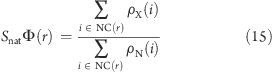where NC(r) is the group of contacts occurring in conformations of the native state for each residue r. S_natΦ(r) usually takes values ranging from 0 to 1 (although values out of this range are also possible), 0 indicating that the structure around residue r is conformationally far from the N state and 1 indicating that the structure is conformationally similar to the N state.

As can be seen in Figure 8, the central residues of the peptide are most native-like, with a general decrease in nativeness toward the terminal residues. The number of contacts formed in the intermediate state is largely independent of temperature, while the transition state becomes less native-like as the temperature is increased. At the lower temperatures, the T state S_natΦ values are larger than those in the I state, indicating a more native-like packing of the side-chains. Figure 8 confirms that the G6–N7 turn sequence is strongly native-like for both the intermediate and transition states at all three temperatures.

Figure 8.

Structural Φ-values per residue in the I and T states at 300, 330, and 360 K.

Discussion

Markov State Model and Markovianity of the TZ1 Representations

The optimized Markov state approach employed here is based on several assumptions whose validity must be considered. The first of these is that the dynamics of the system is Markovian, or memory-less. This implies that the future dynamical evolution of the conformation of a molecule depends only on its current state and not on the previous history of the molecule. In practice, the dynamics of a system is unlikely to be completely Markovian at short time scales,(19) so the mean lifetime of the stable states of a system must be long compared to the length of the memory, allowing fast initial non-Markovian dynamics to be neglected. A preliminary test of the Markovian assumption is based on the convergence of the spectrum of the eigenvalues of the rate matrix, as the lag time is varied. This test showed us that a representation of the system obtained by binning the trajectory along a single observable (the number of native backbone HBs) did not provide Markovian dynamics (as it did in other instances^30,45). This means that the information conveyed by the HB is not sufficient to describe the kinetics of folding of the peptide.

The method was therefore extended to use both HB and rmsd (see Methods), and in this case, the slowest eigenvalues at the three simulation temperatures studied were found to converge for lag times larger than 2.5 ns (Figure 2b). As a further and more stringent test of the Markovian assumption, the decay times of the autocorrelation functions of the first three eigenvectors of R projected along the simulations were examined. Figure 9 shows that these decay times are in good agreement with the decay times expected from the corresponding eigenvalues (Table 1), confirming that this representation is Markovian. The Markovianity of the representation provides a validation, a posteriori, for both the choice of observables (HB and rmsd) and the fine graining of the binning procedure. Indeed, if either of the two was not good enough, then the representation would not be Markovian. We note also that other choices of observables should provide similar slow eigenmodes, as long as the observables report the same amount of information about the slow dynamics of the system.(17)

Figure 9.

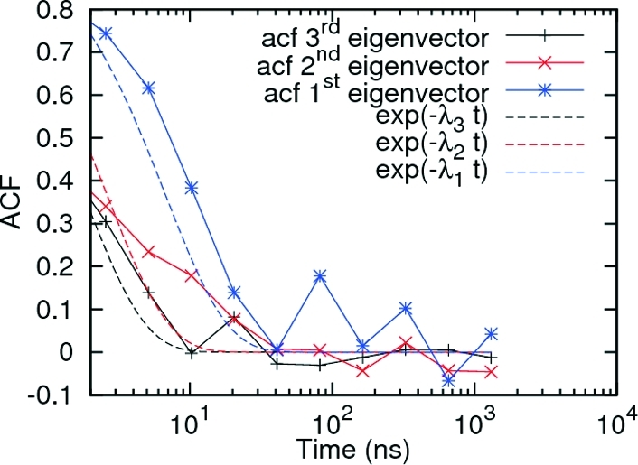
Autocorrelation functions for the first three eigenvectors (continuous lines) of the rate matrix R at 330 K and the corresponding exponential decay associated with the eigenvector (dashed lines). Only data for times larger than lag time are shown.

The Markov States of TZ1

The eigenvector analysis identified three significant relaxation processes, the slowest being the one between the folded and denatured states of the peptide, with relaxation times ranging from 2 to 20 ns, according to the temperature (Table 1). The relaxation times measured in this study cannot be directly compared with experimental data, as the simulations were deliberately run in the absence of solvent viscosity to maximize the number of sampled transition events. However, the 2 orders of magnitude reduction in the transition times measured at 300 K (20.0 ± 0.6 ns, Table 1) with respect to the experimental data (k_obs^–1 = [k_f + k_u]⁻¹ = 4.7 ± 0.3 μs at 296 K(36)) is in line with the reduction observed in a variety of other systems ranging from helices to three-stranded β-hairpin peptides simulated in the same way,⁴⁶⁻⁴⁸ indicating that the force field yields a separation of time scales consistent with experimental data.

Interestingly, the second slowest relaxation, with relaxation times ranging from 1.4 to 4.6 ns (Table 1), occurs between a highly populated, compact state (D1) and a less densely populated state encompassing a broader range of HB and rmsd values (D2). Evidence of this separation of the D1 and D2 states was also indicated in the kinetic network analyses by regions of low link density separating the two (Figure 4). The distance from a pure exponential relaxation for the autocorrelation function of the associated eigenvector (Figure 9) and the presence of a limited overlap (Figure 4) in the kinetic network projection between D1 and D2 states, as reported by the presence of network regions containing clusters from both states, indicates, however, that even the rmsd and HB may be flanked by some other observable to improve the separation between the D1 and D2 states. We also note that, because D1 and D2 may not have been perfectly separated by the HB-rmsd-based MSM, the relaxation times between the two states may be underestimated. These relaxation times are already close to those measured for the main folding transition; thus, we cannot completely exclude the possibility that the D1/D2 exchange occurs via the native state, or, in other words, that the native state represents a kinetic hub connecting the two heterogeneous denatured states as recently proposed for β3s(12) and for villin and NTL9.(49) On the other hand, here the native state is not very stable at any of the simulated temperatures; thus, our system is in a regime where the kinetic hub picture may not necessarily hold. It is plausible that the lack of Markovianity of the representation based only on HB is due to the complexity of the denatured state and the presence of two distinct free energy basins D1 and D2, which cannot be separated by HB alone.

The third significant free energy barrier at 330 and 360 K was found between the N and I states (Figure 2d,e, right), with relaxation times ranging from 0.8 to 1.8 ns (Table 1). This barrier, which is visually more evident from the HB-rmsd projections than the one between D1 and D2, is actually smaller than the latter, as it allows for a faster relaxation (i.e., larger eigenvalue). This is a clear demonstration of the need for a careful kinetic analysis to correctly discriminate the populated macrostates of a biomolecular system, especially when the nature of the stable states is unknown a priori, as in the present case, or in any attempt to characterize the structures of the denatured state. At 300 K, the third relaxation process primarily involves a population exchange between I and D2, with only a weak participation of N (Figure 2c, right), in contrast to what happens at higher temperatures. We note, however, that this result is still sufficient to separate N from I.

The Kinetic Network Analysis Is Necessary to Identify Reactive Species

The disadvantage of using a MSM based on projections of the trajectory upon simple observables (i.e., HB and rmsd) is that the kinetic information contained in the simulation data may be partly lost, an issue that becomes particularly serious when kinetically unstable transition states are considered.(6) The decomposition in macrostates provided by the MSM does not allow for the direct identification of reactive species. Indeed, the distribution of the probability of folding for conformations belonging to the I state shows that I is enriched in reactive conformations with respect to the overall trajectory. However, it also shows that the largest majority of the conformations in I are not reactive (Figure 10). Then, the use of the kinetic network analysis, which allows for the definition of a reliable reaction coordinate, p_commit, becomes necessary for the correct identification of the reactive species.

Figure 10.

Probability density of the commitment probability distribution for state I (continuous line) and for the overall trajectory (dotted line).

The Denatured State

The denatured state of TZ1 in the present simulations appears heterogeneous, because the two substates D1 and D2 have a relatively slow interconversion rate. The state D1 is a compact state where the turn at residues G6 and N7 is formed, while the two strands of the hairpin are not paired by backbone HB and interlocking Trp side chains like the native state but by a disordered arrangement of the Trp side chains in a conformation that possibly minimizes the nonpolar exposure to the solvent. The state D2, on the other hand, is more diffuse and heterogeneous with a lower amount of residual structure, although it retains a certain tendency to form a turn close to residues G6 and N7 (Figure 7). It is worth pointing out that the compact structures with buried tryptophan side chains observed here for the states D1, and to a lesser extent D2, may be the result of an overstabilization of hydrophobic interactions due to the approximate model for the solvent. This may also explain the low population of the native state observed here even at 300 K, in contrast with the experimental midpoint transition temperature of 323 K.(25) Although the comparison with explicit water simulations of the same peptide(22) is made difficult by the different temperatures used in that study, no strong propensity to sample compact conformations in the denatured state was observed in those simulations. Nor were they able to distinguish the two components D1 and D2 of the denatured state, although a further investigation (G.S. unpublished data) revealed that the tendency to form a turn in position 6 and 7 in the denatured state was also present in the explicit water simulations. High temperature explicit water simulations of TZ2,(50) a peptide similar to TZ1 but with a different turn sequence, and an analysis using an automatic Markov state decomposition(13) revealed considerable structure in the denatured state in analogy with what has been found here, although in those studies structure in the denatured state appeared to be stabilized by non-native backbone H-bonds while here it is predominantly stabilized by hydrophobic interaction between tryptophan side chains. Those studies also pointed out the presence of out-of-register hairpin states, some of which are compatible with the N-terminal shift of the turn observed here in some of the conformations of D1.

The Intermediate State

The presence of the significantly populated intermediate state (I) in the current simulations was also observed in explicit-solvent high temperature molecular dynamics simulations of the same peptide,(22) although the detailed structures differ. Indeed, in the present simulations, state I is stabilized by a hydrogen bond between K8 and E5, while, in the explicit water simulations, a hydrogen bond between T3 and T10 was also formed. Previous simulations performed on the related TZ2 peptide led to contrasting results. While large numbers of short implicit-solvent MD simulations suggested a two-state system,(36) other simulations of TZ2 using implicit solvent models(51) favored a noncooperative folding hypothesis, even if the projection of the free energy landscape showed a minimum with characteristics similar to the I state identified in this study. Explicit solvent simulations of TZ2⁵²⁻⁵⁴ also revealed the presence of an intermediate state similar to the I state. Experimental characterization of TZ2 by isotope-edited 2D IR spectroscopy(55) revealed the presence of partially folded states with only the midrange native H-bonds formed along the hairpin, a bulged turn, and variably frayed termini. These conformations resemble the I state identified for TZ1 here and, to a larger extent, that observed in the explicit water simulations.(22) Explicit water simulations of the hairpin B1 from protein G,(56) which has a similar sequence to the trpzip peptides, reported the presence of at least one kinetic intermediate with characteristics similar to the one observed here. The presence of an intermediate state fits the available experimental data on the folding of TZ2 and related peptides, where the unfolding rates are mainly determined by the robustness of the hydrophobic core packing and the folding rates are determined by the turn propensity of the sequence.(57)

The Folding Transition State of TZ1

The transition state T of TZ1 is characterized by a well formed turn region and the proximal part of the strands in extended β-sheet conformation (Figures 6 and 7). With respect to secondary structure content, T is similar to the I state although slightly less native-like. In terms of side chain packing, the T state presents a compact and disordered arrangement of the tryptophan side chains similar to I, although the number of native side-chain contacts in T is larger than in I (Figure 8), indicating the importance of correct side-chain packing for the folding transition to complete. This picture of the transition state is similar to the one obtained from explicit solvent simulations(22) where the rate limiting step for folding was identified in the correct packing of the tryptophan side-chains, while proximal H-bonds and the turn region were already formed at transition.

The structure of the folding transition state was found to be relatively insensitive to changes in temperature in proteins like CI2^58,59 and Protein A.(60) However, smaller structural units such as those represented by small peptides may be more sensitive to environmental changes. While explicit water simulations of the unfolding of the TZ1 peptide(22) showed subtle structural changes in the transition state structures as a function of temperature, the high temperature and lack of proper thermodynamic equilibrium in the simulations prevented a deeper exploration of these phenomena. Here, we observe that the similarity of the T state to the native state N, as reported by the structural Φ values and by the superposition of conformations of T in Figure 6, decreases with temperature. This, however, should not be interpreted as anti-Hammond behavior because this comparison does not take into account the corresponding changes in the denatured state. Indeed, the conformational distribution of N and D1/D2 is also temperature dependent. Experimentally, movements of transition states relative to the ground states are measured in terms of the Tanford beta value,(61) which is thought to approximate the ratio between the solvent accessible surface area buried in T and in N, upon folding from D. Accessible surface area calculations on the conformations identified here as belonging to T, N, and D2 (Table 6) show small differences between the states, relative to the spread of the distributions. This leads to large errors on the determination of the Tanford beta value, which rules out drawing a definitive conclusion about temperature dependent transition state movements. A possible reason for the large error lies in the fact that D2 in our simulations, although less compact than D1, is still a relatively compact state; thus, the change in solvent accessible surface area upon folding is limited.

Table 6. Average Solvent Accessible Surface Area for States D2, N, and T at 300, 330, and 360 K.

	solvent accessible surface area (Å2)
temperature (K)	N	T	D2
300	1410 ± 40	1460 ± 50	1470 ± 80
330	1430 ± 50	1500 ± 70	1490 ± 80
360	1460 ± 60	1500 ± 70	1530 ± 80

Conclusions

Here, we showed how the combined use of MSM analysis and kinetic network analysis allows for a detailed, concise, and consistent characterization of both the metastable and the transition states for folding of peptides. Besides states identified in earlier simulations, the Markov state analysis of trajectories projected on standard observables allowed for the identification of different subspecies in the denatured state of the TZ1 peptide, which could otherwise be easily missed by standard inspection of the projected trajectory. The metastable states as identified by the Markov state analysis provided a solid base to perform approximate commitment probability calculations using the kinetic network representation of the peptide dynamics and correctly identify the reactive species. The approximate commitment probabilities were proven to represent a good reaction variable. The Markov state analysis and the kinetic network analysis also provided a consistent reciprocal validation of the results, showing that the Markov macrostates are kinetically localized and well partitioned along the network. The picture of the folding process of TZ1 emerging from the analysis is the following. The slowest conformational change observed in TZ1 is the conversion between folded and denatured species. The other slow processes involve exchange between a compact and a less compact subspecies of the denatured state and exchange between the fully native and partially folded intermediate state with an H-bond formed close to the turn. The transition state for the slowest relaxation process (i.e., folding) is characterized by the formation of H-bonds proximal to the turn and a well structured turn region, while packing of the tryptophan side-chains is not complete, although it encompasses more native contacts than in the intermediate state.

Author Present Address

^† Institute of Physics, University of Mainz, Germany.

References

- Bryngelson J. D.; Onuchic J. N.; Socci N. D.; Wolynes P. G. Proteins 1995, 21, 167. [DOI] [PubMed] [Google Scholar]
- Bryngelson J. D.; Wolynes P. G. Proc. Natl. Acad. Sci. U.S.A. 1987, 84, 7524. [DOI] [PMC free article] [PubMed] [Google Scholar]
- Onuchic J. N.; Wolynes P. G.; Luthey-Schulten Z.; Socci N. D. Proc. Natl. Acad. Sci. U.S.A. 1995, 92, 3626. [DOI] [PMC free article] [PubMed] [Google Scholar]
- Wang J.; Onuchic J.; Wolynes P. Phys. Rev. Lett. 1996, 76, 4861. [DOI] [PubMed] [Google Scholar]
- Daggett V.; Li A. J.; Itzhaki L. S.; Otzen D. E.; Fersht A. R. J. Mol. Biol. 1996, 257, 430. [DOI] [PubMed] [Google Scholar]
- Rao F.; Settanni G.; Caflisch A. Methods Mol. Biol. 2007, 350, 225. [DOI] [PubMed] [Google Scholar]
- Das P.; Moll M.; Stamati H.; Kavraki L. E.; Clementi C. Proc. Natl. Acad. Sci. U.S.A. 2006, 103, 9885. [DOI] [PMC free article] [PubMed] [Google Scholar]
- Singhal N.; Snow C. D.; Pande V. S. J. Chem. Phys. 2004, 121, 415. [DOI] [PubMed] [Google Scholar]
- Rao F.; Caflisch A. J. Mol. Biol. 2004, 342, 299. [DOI] [PubMed] [Google Scholar]
- Settanni G.; Rao F.; Caflisch A. Proc. Natl. Acad. Sci. U.S.A. 2005, 102, 628. [DOI] [PMC free article] [PubMed] [Google Scholar]
- Rao F.; Settanni G.; Guarnera E.; Caflisch A. J. Chem. Phys. 2005, 122, 184901. [DOI] [PubMed] [Google Scholar]
- Krivov S. V.; Muff S.; Caflisch A.; Karplus M. J. Phys. Chem. B 2008, 112, 8701. [DOI] [PMC free article] [PubMed] [Google Scholar]
- Chodera J. D.; Singhal N.; Pande V. S.; Dill K. A.; Swope W. C. J. Chem. Phys. 2007, 126, 155101. [DOI] [PubMed] [Google Scholar]
- Noe F.; Horenko I.; Schutte C.; Smith J. C. J. Chem. Phys. 2007, 126, 155102. [DOI] [PubMed] [Google Scholar]
- Gfeller D.; De Los Rios P.; Caflisch A.; Rao F. Proc. Natl. Acad. Sci. U.S.A. 2007, 104, 1817. [DOI] [PMC free article] [PubMed] [Google Scholar]
- Ozkan S. B.; Dill K. A.; Bahar I. Biopolymers 2003, 68, 35. [DOI] [PubMed] [Google Scholar]
- Swope W. C.; Pitera J. W.; Suits F. J. Phys. Chem. B 2004, 108, 6571. [Google Scholar]
- Sriraman S.; Kevrekidis I. G.; Hummer G. J. Phys. Chem. B 2005, 109, 6479. [DOI] [PubMed] [Google Scholar]
- Buchete N. V.; Hummer G. J. Phys. Chem. B 2008, 112, 6057. [DOI] [PubMed] [Google Scholar]
- Noe F.; Schutte C.; Vanden-Eijnden E.; Reich L.; Weikl T. R. Proc. Natl. Acad. Sci. U.S.A. 2009, 106, 19011. [DOI] [PMC free article] [PubMed] [Google Scholar]
- Bowman G. R.; Huang X.; Pande V. S. Methods 2009, 49, 197. [DOI] [PMC free article] [PubMed] [Google Scholar]
- Settanni G.; Fersht A. R. Biophys. J. 2008, 94, 4444. [DOI] [PMC free article] [PubMed] [Google Scholar]
- Fink A. L. Curr. Opin. Struct. Biol. 2005, 15, 35. [DOI] [PubMed] [Google Scholar]
- Sanchez I. E.; Kiefhaber T. J. Mol. Biol. 2003, 327, 867. [DOI] [PubMed] [Google Scholar]
- Cochran A. G.; Skelton N. J.; Starovasnik M. A. Proc. Natl. Acad. Sci. U.S.A. 2001, 98, 5578. [DOI] [PMC free article] [PubMed] [Google Scholar]
- Brooks B. R.; Bruccoleri R. E.; Olafson B. D.; States D. J.; Swaminathan S.; Karplus M. J. Comput. Chem. 1983, 4, 187. [Google Scholar]
- Ferrara P.; Apostolakis J.; Caflisch A. Proteins 2002, 46, 24. [DOI] [PubMed] [Google Scholar]
- Berendsen H. J. C.; Postma J. P. M.; Vangunsteren W. F.; Dinola A.; Haak J. R. J. Chem. Phys. 1984, 81, 3684. [Google Scholar]
- Ryckaert J. P.; Ciccotti G.; Berendsen H. J. C. J Comput. Phys. 1977, 23, 327. [Google Scholar]
- Hummer G. New J. Phys. 2005, 7. [Google Scholar]
- Deuflhard P.; Huisinga W.; Fischer A.; Schütte C. Linear Algebra Appl. 2000, 315, 39. [Google Scholar]
- Deuflhard P.; Weber M. Linear Algebra Appl. 2005, 398, 161. [Google Scholar]
- Hartigan J. A.Clustering Algorithms; John Wiley & Sons, Inc.: New York, 1975. [Google Scholar]
- Seeber M.; Cecchini M.; Rao F.; Settanni G.; Caflisch A. Bioinformatics 2007, 23, 2625. [DOI] [PubMed] [Google Scholar]
- Du R.; Pande V. S.; Grosberg A. Y.; Tanaka T.; Shakhnovich E. S. J. Chem. Phys. 1998, 108, 334. [Google Scholar]
- Snow C. D.; Qiu L.; Du D.; Gai F.; Hagen S. J.; Pande V. S. Proc. Natl. Acad. Sci. U.S.A. 2004, 101, 4077. [DOI] [PMC free article] [PubMed] [Google Scholar]
- Hummer G. J. Chem. Phys. 2004, 120, 516. [DOI] [PubMed] [Google Scholar]
- Brandes U.; Wagner D.. Visone - Analysis and visualization of social networks. In Graph Drawing Software; Jünger M., Mutzel P., Eds.; Springer: Berlin, 2003; p 321. [Google Scholar]
- Zheng W.; Gallicchio E.; Deng N.; Andrec M.; Levy R. M. J. Phys. Chem. B 2011, 115, 1512. [DOI] [PMC free article] [PubMed] [Google Scholar]
- Best R. B.; Hummer G. Proc. Natl. Acad. Sci. U.S.A. 2005, 102, 6732. [DOI] [PMC free article] [PubMed] [Google Scholar]
- Best R. B.; Hummer G. Proc. Natl. Acad. Sci. U.S.A. 2010, 107, 1088. [DOI] [PMC free article] [PubMed] [Google Scholar]
- Frishman D.; Argos P. Proteins 1995, 23, 566. [DOI] [PubMed] [Google Scholar]
- Humphrey W.; Dalke A.; Schulten K. J. Mol. Graphics 1996, 14, 33. [DOI] [PubMed] [Google Scholar]
- Li A. J.; Daggett V. J. Mol. Biol. 1996, 257, 412. [DOI] [PubMed] [Google Scholar]
- Best R. B.; Hummer G. Phys. Rev. Lett. 2006, 96, 228104. [DOI] [PubMed] [Google Scholar]
- Ferrara P.; Apostolakis J.; Caflisch A. J. Phys. Chem. B 2000, 104, 5000. [Google Scholar]
- Cavalli A.; Ferrara P.; Caflisch A. Proteins 2002, 47, 305. [DOI] [PubMed] [Google Scholar]
- Cavalli A.; Haberthur U.; Paci E.; Caflisch A. Protein Sci. 2003, 12, 1801. [DOI] [PMC free article] [PubMed] [Google Scholar]
- Bowman G. R.; Pande V. S. Proc. Natl. Acad. Sci. U.S.A. 2010, 107, 10890. [DOI] [PMC free article] [PubMed] [Google Scholar]
- Pitera J. W.; Haque I.; Swope W. C. J. Chem. Phys. 2006, 124. [DOI] [PubMed] [Google Scholar]
- Yang W. Y.; Pitera J. W.; Swope W. C.; Gruebele M. J. Mol. Biol. 2004, 336, 241. [DOI] [PubMed] [Google Scholar]
- Zhang J.; Qin M.; Wang W. Proteins 2006, 62, 672. [DOI] [PubMed] [Google Scholar]
- Nymeyer H. J. Phys. Chem. B 2009, 113, 8288. [DOI] [PubMed] [Google Scholar]
- Kim J.; Keiderling T. A. J. Phys. Chem. B 2010, 114, 8494. [DOI] [PubMed] [Google Scholar]
- Smith A. W.; Lessing J.; Ganim Z.; Peng C. S.; Tokmakoff A.; Roy S.; Jansen T. L.; Knoester J. J. Phys. Chem. B 2010, 114, 10913. [DOI] [PubMed] [Google Scholar]
- Bolhuis P. G. Proc. Natl. Acad. Sci. U.S.A. 2003, 100, 12129. [DOI] [PMC free article] [PubMed] [Google Scholar]
- Du D.; Zhu Y.; Huang C. Y.; Gai F. Proc. Natl. Acad. Sci. U.S.A. 2004, 101, 15915. [DOI] [PMC free article] [PubMed] [Google Scholar]
- Tan Y. J.; Oliveberg M.; Fersht A. R. J. Mol. Biol. 1996, 264, 377. [DOI] [PubMed] [Google Scholar]
- Day R.; Daggett V. Protein Sci. 2005, 14, 1242. [DOI] [PMC free article] [PubMed] [Google Scholar]
- Sato S.; Fersht A. R. J. Mol. Biol. 2007, 372, 254. [DOI] [PubMed] [Google Scholar]
- Fersht A. R.Structure and Mechanism in Protein Science; W. H. Freeman: New York, 1999. [Google Scholar]