Detecting Selective Expression of Genes and Proteins

Abstract

Selective expression of a gene product (mRNA or protein) is a pattern in which the expression is markedly high, or markedly low, in one particular tissue compared with its level in other tissues or sources. We present a computational method for the identification of such patterns. The method combines assessments of the reliability of expression quantitation with a statistical test of expression distribution patterns. The method is applicable to small studies or to data mining of abundance data from expression databases, whether mRNA or protein. Though the method was developed originally for gene-expression analyses, the computational method is, in fact, rather general. It is well suited for the identification of exceptional values in many sorts of intensity data, even noisy data, for which assessments of confidences in the sources of the intensities are available. Moreover, the method is indifferent as to whether the intensities are experimentally or computationally derived. We show details of the general method and examples of computational results on gene abundance data.

It is well established that a eukaryotic cell’s genomic DNA and expressed mRNA are present in a variety of abundance classes (Britten and Kohn 1968; Galau et al. 1977; Hames and Higgins 1985). Very wide differences in gene expression level, that is, in intracellular mRNA copy number or in amount of gene product, are possible within the same cell. For example, it has been estimated that the copy numbers of expressed genes can vary from 1 to ∼200,000 (Patanjali et al. 1991). For many genes, such differences in abundances can be detected coarsely through experimental rehybridization kinetics or can be estimated from the rates of protein synthesis of specific enzymes (Galau et al. 1977). More modern abundance detection techniques are also available (Singer and Berg 1991; Adams 1994; Wilkins et al. 1997). The same cell type, as well as different cell types, may exhibit different patterns of gene expression when exposed to different conditions (Singer and Berg 1991; Adams 1994; Lodish et al. 1995; Wilkins et al. 1997). Assessing differences in expression patterns, therefore, can be used to gauge differences in cell physiology and tissue behavior, intrinsically or in response to many different kinds of stimuli.

Because gene expression is central to modern biology, it is expected that delineations of patterns of gene or protein expression among normal and diseased states will have increasing importance in medical diagnostics and therapy (Anderson et al. 1984; Anderson and Seilhamer 1997). The conjunction of large-scale biology technologies (e.g., genomic sequencing or proteomics) and the need for new pharmaceutical targets has motivated the development of computational methods for detecting unusual expression patterns. Among the patterns of interest is selective expression, in which the expression (mRNA or protein) in a specific tissue is at a significantly different level than the other tissues. Selective expression is of particular interest because it may be correlated with fundamental biological phenomena or disease processes.

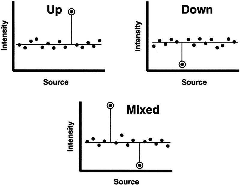
Two stereotypical selective expression situations are possible: up, in which expression is elevated in a specific tissue when compared with the levels in other tissues; and down, in which the expression in a specific tissue is reduced significantly when compared with the levels in other tissues. Although mixed situations are possible, they will not be discussed in this article (see Fig. 1 for diagrammatic representations). The extension of the techniques for identifying up or down selective expression to the mixed cases is straightforward.

Figure 1.

Selective expression types. Examples of selective expression stereotypes—up, down, and mixed—are diagrammed. Intensities vs. sources from a source set are plotted in arbitrary order. In each diagram, it is presumed that the outstanding intensities are exceptionally large or exceptionally small, when compared against the other intensities; hence, selective expression. Selectively expressed intensities are indicated by encircled symbols.

Up selective expression may be an important indication that the gene has been activated specifically, up-regulated, or its product elevated differentially in association with certain phenomena or agents affecting a particular tissue’s biology. Similarly, down selective expression is either a significant down-regulation or a nearly complete inactivation of the gene (e.g., tumor-suppressor loss of function) in association with specific biological events. Such broad phenomena as morphogenesis, differentiation, metabolic alteration, mutagenesis, bacterial and viral infection, physiological stress, disease, drugs and therapeutic interventions, etc. can manifest or cause selective expression effects. A particular example at SmithKline Beecham Pharmaceuticals was the discovery of a novel cathepsin gene (cathepsin K) being selectively up-expressed in an osteoclast library and subsequently shown to be involved in bone resorption (Bossard et al. 1996; Drake et al. 1996; Zhao et al. 1997). This experimental finding significantly motivated the development of this selective expression detection computational method.

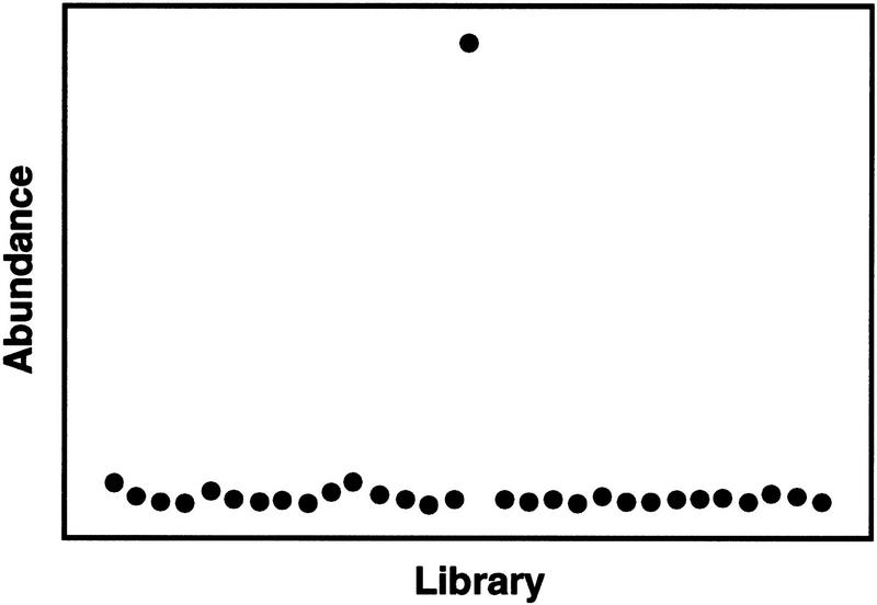
This article presents a robust computational method that identifies genes or proteins that are expressed selectively (see Fig. 2 for a representation of selective expression in real data). The method is not restricted to gene or protein expression data, though such expression data is among the more natural contexts for this approach. The method is generally applicable to any kind of intensity data in which a distinguishable data source (e.g., tissue, library, assay, drug, dose, time, etc.) can be associated with each intensity value (e.g., gene or protein abundance, activity, binding strength, fluorescence, etc.). If assessments of reliabilities, that is, confidences, in the sources are available, these can be utilized to make more reliable predictions. The intensities can be experimentally determined values, computationally derived values [e.g., from expressed sequence tag (EST) data (Myers 1994)], or combinations. The method is indifferent to the experimental or computational lineages of the data to be analyzed. All that is required are triples of associated values: intensity, source, and source confidence. Conveniently, a set of values can be organized generally as a two-dimensional matrix of intensities, in which each column corresponds to each source (with its associated source confidence), and each row corresponds to each entity for which intensities are assessed, for example, intensity in row versus column, corresponding respectively to abundance of gene versus library, binding strength of drug versus tissue, biological activity of drug versus dose, and so forth. The method is applicable as well to intensities from the same source (column), for example, different genes’ abundances (row) in a particular library (column), binding strength of different drugs (row) in the same tissue (column), biological activity of different drugs (row) at the same dose in the same tissue (column).

Figure 2.

Selective expression example from real data. The results shown in this example are for an actual assembly, which is highly homologous to mRNA for a 23-kD highly basic protein. Intensities (abundances) are plotted vs. sources (libraries) in arbitrary order. The single exceptionally large intensity compared to the other intensities in the source set was detected by the algorithm as a strong selective expression.

Foundations

Before presenting the approach, we delineate four essential concepts to provide a conceptual footing for the selective expression identification method:

1. “Intensity” is a non-negative numerical quantity that is representative of the phenomenon of interest. For example, intensity could be a drug’s binding affinity, a compound’s activity in a screen, or a gene’s “abundance,” such as the gene product’s copy number (molecules or concentration of mRNA) or amount of protein expressed, and so forth. Intensity can be either an experimentally measured quantity or a quantity that is calculated from analyses of EST assemblies. [Assemblies are computational constructs comprising EST components from sequenced libraries that have been combined to represent putative genes (Adams et al. 1994; Burks et al. 1994; Myers 1994).]

2. “Source” is the identification of the source of the “intensity” data. It can be, for example, a cDNA library or a tissue that provides a set of expression intensity or abundance values (Anderson et al. 1984; Adams et al. 1994; Anderson and Seilhamer 1997) of the genes being compared. If a source is manipulated experimentally or edited in any way, for example, a subtracted or normalized cDNA library, it should not be included in the analysis lest its pattern of expressed genes is artificially skewed. This exclusion principle can be relaxed if all the sources being compared have been manipulated in the same way.

   In general, sources are considered independent of each other with no intrinsic ordering. However, this is not always true when the sources can be ranked according to an external experimentally controlled variable, e.g., time, age, dose, disease staging, treatment concentration, etc. In these situations it is natural, although not required, to order the sources by ascending control variable values.

3. “Source set” comprises a subset of the sources among which intensities can be compared. In particular, selective expression is a marked difference of intensity in a single source from a baseline level of expression established by the gene’s intensities in a particular source set (see Fig. 1 for stereotypical examples). The selective expression concept does not require, however, that comparisons be made against all known sources. Instead, a carefully chosen subset of the known sources can be considered, especially as selective expression is a relative, not an absolute, assessment. Care must be exercised in choosing source sets so as not to bias the selective expression prediction. Recognizing this, choice of source set enables the biological context for expression comparisons to be tailored to the biological questions being asked—organ systems versus one another, tissues versus one another (e.g., endothelium versus smooth muscle or fibroblast), drug dose responses versus one another, effects of compounds versus one another, human versus nonhuman species, and so forth. It is the careful matching of source set to the relevant biological question that should minimize artifactual biases being introduced.

   All the intensities from the same source are scaled by the source’s maximum observed intensity. This is done to make intensities from different sources within the source set commensurably comparable, which is necessary if intensity patterns across sources are to be identified.

4. “Source confidence” represents the quality, reliability, and knowledge of error or the relative trust that can be attributed to the source. When source confidences are quantitated in some fashion, we call them “source quality weights.” For example, a larger weight would be associated with a carefully harvested and rapidly preserved tissue (high quality) than with a poorly captured or slowly preserved one (low quality). A cDNA library sequenced in depth is a more reliable source, hence has a larger weight, than the same library sequenced to a lesser depth. An edited or normalized cDNA library should be considered a low confidence source unless all the sources in the source set have been manipulated equivalently. We note that any consistent source quality weighting scheme can be used, but care must be exercised. If the weights are not faithful to the reliabilities of the sources, any results dependent upon them may be improperly distorted. As explained in the Algorithm and Details sections (below), a selective expression assessment can take into account the weights of the different sources constituting the source set.

The focus of this work is not on the molecular details of the processes of gene expression or protein synthesis. Rather, we are interested in comparing relative levels of mRNA transcripts or protein products. Despite the inherent difficulties in measuring precisely which mRNA species are translated and in what relative proportions, reliable enough information on expression levels can be obtained (Adams 1994; Anderson and Seilhamer 1997; Herbert et al. 1997). Moreover, the established experimental techniques of cDNA and EST sequencing, especially when employed on a large scale, can provide ESTs that can be combined computationally into assemblies (Adams et al. 1994). Assemblies can be interpreted as putative expressed genes, though with widely varying levels of confidence in the assignments to genes (Burks et al. 1994; Myers 1994). Abundances of expressed genes or assemblies obtained from sampling are dependent on the depth of the sampling (Lewins and Joanes 1984; Bunge and Fitzpatrick 1993) and contribute to inaccuracies in the computed intensities (Myers 1994). We note that this sampling depth issue (Audic and Claverie 1997) can be viewed as a source reliability problem.

Statistical Considerations

In general, the problem of identifying selectively expressed intensities in multisource data can be viewed as an outlier identification problem in a different guise. We choose to adopt the view of outlier employed by Barnett and Lewis (1978a) and others (Grubbs 1969): “But what characterizes the ’outlier’ is its impact on the observer (it appears extreme in some way)” (Barnett and Lewis 1978b). Identification of an outlying intensity is not the endpoint of the analysis. Rather, statistical outlier identification is one component of a larger analysis scheme that includes additional (e.g., biological) considerations.

Statistical objectivity can be introduced through the concept of discordancy: “... an observation will be termed discordant if it is statistically unreasonable on the basis of some prescribed probability model.” (Barnett and Lewis 1978c). This relies on choosing a probability model for the data so quantitative assessments of outliers against the model can be done. We choose to interpret a resulting discordancy significance probability as a relative strength of confidence in the statistical identification. An advantage of this interpretation is that it makes it possible to consistently order the results from statistically insignificant, to weak, to strong. Thus, the rank order of the relative confidences of identification is preserved. This confidence ordering is critical because there is little knowledge of the extent to which the statistical test’s probability model may be inappropriate.

At the current state of biological understanding, the actual form of any underlying probability distribution (if one exists at all) is entirely unknown (Singer and Berg 1991; Lewin 1994). Moreover, even if the concept of an underlying intra-source intensity distribution is appropriate, very little can be said about distributions that may be governing inter-source intensity comparisons. Nonetheless, it could be assumed that certain distributions can reasonably describe inter-source intensity comparisons. Because intensities are nonnegative, well-known distributions on the nonnegative real axis could be chosen, e.g., exponential, gamma, log normal. However, the discordancy tests associated with these distributions suffer from the necessity to estimate parameters (Barnett and Lewis 1978a). Neither the available intensity data nor theoretical knowledge support the estimation of distribution parameters in this inter-source sampling problem. As expression intensities are bounded, a practical way exists for the choice of a distribution: Assume a distribution defined on a finite domain, whose shape is simple, and for which a discordancy test independent of the distribution’s parameters is available. The Dixon discordancy test for uniform distributions meets these criteria (Barnett and Lewis 1978a). Uniform is a reasonable choice because it confers only a very weak bias in distribution shape or in central tendency. How we employ this test for selective expression is described in the Details subsection of Results.

Outline of the Selective Expression Algorithm

The previous discussions have set the stage for the identification of selective expression in data comprising triples: intensity, source, and source quality weight. First, an overview of the algorithm is given. Then, the mathematical details of the key steps (steps 4–7) are explained in the Details section.

Step 1—Minimum Source Quality Criterion

For an entity’s collection of intensities to be analyzed from the source set (e.g., a particular gene’s abundances in a source set of libraries), select the intensities from only those sources whose corresponding quality (i.e., trust, reliability, or relevance) exceeds a minimum threshold. Because the method seeks to identify an entity’s exceptional intensity in a source set, it would make trifling sense to attempt such an identification when there is not at least a minimal quality met by the individual sources. Though there is no intrinsic method for setting a minimum quality threshold, scientific judgments concerning the reliabilities or relevances of the sources and the nature of weighting schemes can be used to make this determination. Often, as data are being accumulated, a source’s quality will change with the data collected, requiring the selective expression algorithm to be reapplied.

Step 2—Minimum Number of Sources Criterion

There must be at least a predetermined minimum number of intensities, for example, 10, surviving step 1, each of which exceeds appropriate detection limits (discussed below). If this occurs, continue with further analysis. Generally, it is not possible, practically or theoretically, to reliably identify exceptional values in data sets that have too few elements (Barnett and Lewis 1978a; Hawkins 1980). In practice, we consider 10 to be a prudent minimum number of intensities, i.e., enough to make confident identifications of exceptional intensities. However, a number below 10 (but more than two) can be analyzed for discordancy, if one is willing to accept lower confidences in the assessments (Barnett and Lewis 1978a). Plots of theoretical statistical significance of discordancy (such as Figs. 3 and 4, which are discussed in Details) can show the rate at which statistical significance degrades with decreasing source set sample size.

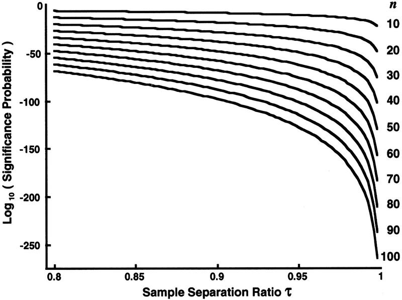
Figure 3.

Dependence of the Dixon theoretical statistical significance probabilities on the sample separation ratio at fixed number of samples taken. The logarithms of the Dixon theoretical statistical significance probabilities for discordancy in uniform samples (Barnett and Lewis 1978a) are plotted against the sample separation ratio τ ε [0.8, 0.995], (equations 1–6). Each theoretical curve (right) is at a different fixed number n of samples, n = [10, 20, ... , 100], respectively. τ near 1 reflects a largest sample being widely separated from the next largest sample when compared to the separation of the largest and smallest samples (see Fig. 6).

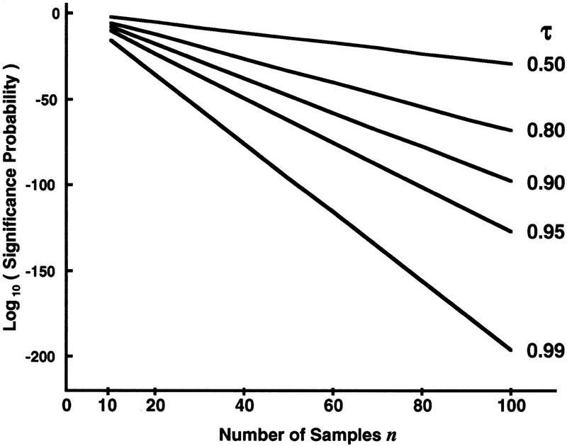
Figure 4.

Dependence of Dixon theoretical statistical significance probabilities on the number of samples taken at fixed separation ratios. The logarithms of the Dixon test theoretical statistical significance probabilities (equation 6) are plotted against the number of points n in a sample, [10, 11, ... , 100]. Each theoretical line (right) is at a different fixed sample separation ratio τ = [0.5, 0.8, 0.9, 0.95, 0.99], respectively. From the family of lines, the rapid decrease in statistical significance probability with increasing sample size n is apparent. This effect is stronger the closer τ is to unity.

Several points should be made concerning intensity detection limits. If an intensity appears to be absent from a particular source, then either (1) the intensity is actually not expressed in the source, or (2) the intensity is indeed expressed but is smaller than the minimum intensity that can be measured, the detection limit. In the second case, because the intensity is not truly absent but instead occurs below the detection limit, it is recorded as absent. However, trusting an absent intensity amounts to accepting point 1 as the explanation over point 2. To decide quantitatively to trust an intensity as being absent from a source, that is, how to trust “absence of evidence as evidence of absence,” is outside the algorithm being discussed even though this issue is intrinsically linked to the issue of source quality. The general problem of estimating confidences of unobserved events has a long history in the statistical literature, yet remains unwieldy (Robbins 1968; Bunge and Fitzpatrick 1993). Adopting a philosophy that maintains that absent intensities can be trusted as genuine absence seems prudent only for very high quality sources with very low detection limits. This is the philosophy we adopt in practice, and all absent or subdetection limit intensities are therefore ignored. This has the effect of being overly conservative in the direction of generating too many false negatives. However, the method does not require adopting this philosophy.

Step 3—Discordancy Statistical Test

The quantitative identification of exceptional intensities occurs in this step. Apply a statistical test of discordancy (Barnett and Lewis 1978a), which may employ the source qualities from step 2, as a means to identify an exceptional intensity. Use the resulting statistical significance to score how exceptional the putative discordant intensity is. The mathematical details of the discordancy test and how the source quality weights are incorporated are explained in the Details section. We note that the method is applicable to exceptionally small intensities (down-selective expression) as well as exceptionally large intensities. The subsequent discussions focus on the exceptionally large intensity case (up-selective expression) to frame ideas. The down case will be discussed in Details.

Step 4—Adjustment Due to Intensity Baseline

Apart from the putative discordant intensity, the other intensities among those being compared can be characterized as being clustered about a baseline level (see Fig. 5, which is discussed further in Details, for illustrations of the effects of different baseline positions). Adjust the step 3 statistical test of discordancy according to the difference between the baseline position and the maximum allowed intensity. The adjustment to the statistical significance is to increasingly downgrade it as the baseline becomes closer to the maximum allowed intensity. The motivation and reasoning behind the baseline-dependent adjustment is based on the dynamic range of the values being increasingly compressed, hence less mutually distinguishable, the closer the baseline is to the allowed upper limit. Because the discrimination of values is necessarily eroded as the effective dynamic range is compressed, the confidence in outlier detection should be eroded correspondingly. This is explained further with an illustrative example in Details.

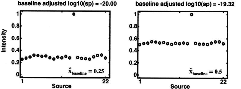
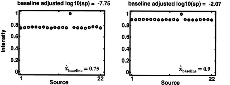
Figure 5.

Discordancy statistical significance adjusted for baseline position. Synthetic intensity data vs. source for several different baselines, [0.25, 0.5, 0.75, and 0.9], are plotted. In each case, the number of samples (n = 22), the maximum intensity (x_n = 1), and the traditional Dixon significance probability [log₁₀(sp) = −20] are kept fixed. Constant Dixon statistical significance, regardless of baseline position, is achieved deliberately in these synthetic data by adjusting x_n −1 according to equations 1–6. Hence, the gap (x_n − x_n − 1) necessarily decreases as the baseline increases; yet, the traditional Dixon statistical significance remains unchanged. The closer the baseline is to the maximum allowed intensity (i.e., 1), the less statistical confidence we can have in an outlier assessment. As can be seen in each panel, the baseline adjusted statistical significance decreases as the baseline increases toward the allowed maximum. The erosion of statistical confidence from the traditional Dixon significance as baselines are continuously increased toward the allowed maximum is plotted in Fig. 7 (see also Table 1).

Step 5—Minimum Intensity Gap Criterion

A fundamental ingredient in discordancy assessment is the separation between the largest and the next-to-largest intensities, which we call the gap (see Fig. 6 and Details step 3). If the gap is below or near the resolving power of the technique providing the intensity data, there is a necessarily negligible confidence in the assessment of discordancy, regardless of the discordancy statistical significance. This is because a gap commensurable with the intensity measurement technique’s resolving power means that the difference between the values constituting the gap is indistinguishable from measurement noise. Therefore, a minimum gap criterion should be applied in conjunction with the discordancy statistical test from step 4. Whereas there is no objective formula for establishing the minimum gap criterion, scientific judgment can be used to set the minimum gap threshold that takes into account the accuracy and resolving power of the technique that provides the intensity data.

Figure 6.

Separation of a largest value from the others and the basic measures for the Dixon test. This diagram displays the separation of a largest value from the others when the values being compared are sorted from smallest to largest, x_i − 1 ⩽ x_i. The separation ratio τ, is the distance between the largest and the next-to-largest values (gap = x_n − x_n − 1) divided by the distance between the largest and smallest values (x_n − x₁). The ratio τ is fundamental in the Dixon test for discordancy (Barnett and Lewis 1978a), which assesses statistically how exceptionally large the largest value is compared to the others. See equations 1–6 in Algorithm Details. In the examples, f_max = 1.

Step 6—Overall Confidence in Selective Expression Determination

The gap from step 5 should be combined with the baseline adjusted statistical significance of discordancy from step 4 to provide an overall confidence of selective expression. This is accomplished by applying a decision function of both the baseline adjusted statistical significance and the gap. The decision function ranks the assessment into low (weak), medium (moderate), or high (strong) confidence of selective expression. However, if either a minimum baseline adjusted discordancy significance was not met or a minimum gap was not exceeded, then selective expression is not considered as being exhibited. How such a decision function is constructed and employed is explained in Details.

We note that there is no intrinsic method to determine the mathematical forms of decision functions. Even if there were such, the situation would still remain that there is no intrinsic objective technique to determine what separates the overall confidences, weak from strong. Nonetheless, there is practical utility in assigning confidences, however imperfectly, to separate weak from strong predictions of selective expression. An interpretation of the strength of a result is often used for setting priorities for further analyses of the data or new experiments.

RESULTS

Here we present the mathematical details of the algorithms’s key steps (3, 4, and 6), as well as examples of the algorithm applied to synthetic and real data.

Details of the Key Steps of the Algorithm

Step 3—The Discordancy Test for Identifying Exceptional Intensities

As discussed in Statistical Considerations (above), we choose a Dixon test (Barnett and Lewis 1978a) for the statistical test of discordancy among the sources being compared within the source set. Further comments are warranted concerning the Dixon test. The first graph in Figure 1 diagrammatically shows a source set of intensities having a single exceptionally large intensity. Such data can be sorted in ascending order and replotted as in Figure 6. When values are sorted, the relative separation between the largest value and the remaining values becomes clearer. [We note that it is common practice for various analysis purposes such as assessing extremes, determining likelihoods of exceptional values occurring, distinguishing populations, etc., to order the elements of data sets sequentially when the data are intrinsically unordered or nonsequentially related (Gumbel 1958; Barnett and Lewis 1978a; Sachs 1982; Poschel et al. 1995).] The size of the gap between the largest and next largest value divided by the distance between the largest and smallest values (see Fig. 6) is an obvious measure of the separation of the largest value from all the other values. This separation ratio (equation 4 below) is the core of the statistic employed in the Dixon test for a single largest discordant value among uniform samples (Barnett and Lewis 1978a). It captures the logical underpinnings of the test.

We consider as well the more general Dixon test for the m^th largest discordant value in a set of n uniform samples (1 ⩽ m < n). However, for application to selective expression, the single largest value test (m = 1) is sufficient. Hence, the mathematical details for only the single largest value form of the Dixon test are presented. In the case of the more general m^th largest discordant value Dixon test, the appropriate changes in the formulas for the degrees of freedom and the separation ratio-dependent statistic (Barnett and Lewis 1978a) can be employed. The more general case is applicable to the problem of simultaneously identifying more than one selectively expressed intensity in a collection of intensities.

Step 3—Mathematical Details

For a selected entity (e.g., gene), let the vector f′ comprise the intensities from the n different sources of the source set which are to be analyzed after step 2. Let q be the vector comprising the corresponding source quality weights from step 2. The elements of f′ and q are real numbers ≥0. The sequential order of the vectors’ elements is arbitrary as the order of the sources in the source set can be arbitrary. However, once an order of sources is chosen, the elements of f′ and of q must appear in the same order, as the respective correspondences between qualities and sources must be maintained. Define vectors f and f_down from f′ as follows:

1a

1b

1c

{f′} represents all the intensities that could occur in the source set. Thus, f_max is the maximum possible intensity that can be observed in principle over the source set. This can be based on either experimental considerations (e.g., maximum signal possible from the intensity measuring instrument) or on how the intensity data are chosen to be normalized. When, for example, the intensities from a source represent gene-expression abundances as a fraction of total genes that could be expressed in a source, the maximum possible intensity is 1. Typically, we take f_max = 1, and this is used in the examples. However, it may not be possible to know the maximum in principle, in which case the maximum observed in the source set will do for f_max.

We note that essentially the same method that is used for the identification of exceptionally large intensities (i.e., up-selective expression) can be employed with minor modifications for the identification of exceptionally small intensities (i.e., down-selective expression). For down-selective expression, replace the vector f (equation 1b) throughout the following discussion by the vector f_down (equation 1c). Though the mathematical form of the algorithm is unchanged by using f_down in place of f, identifying exceptionally small values is fundamentally, and practically, different from identifying exceptionally large values. This is because there can be intensities in f that are so minute (though still above a very small detection limit) as to be measurements indistinguishable from noise, making them useless as reliable values in a discordancy test. One way to remedy this difficulty is to restrict f to comprise only those values that are considerably larger than the detection limit. However, once equation 1b is used, the same baseline adjustment technique used for f (step 4) can be applied to f_down.

Define x as the vector that comprises the n elements of f sorted in ascending order, that is, x_i − 1 ⩽ x_i. Next, compute the Dixon critical statistic t_critical from the elements of x (equations 3–5, below). Then use the Dixon test (equation 2, below) to compute the discordancy significance probability of the largest intensity among these intensities being compared.

According to the Dixon test for a single largest value in n independent samples of a uniform random variable (Barnett and Lewis 1978a), the significance probability (sp) that the largest sample is discordant, that is, exceptionally large, is given by

2

where P is probability; t represents any possible value of (n − 2)τ/(1 − τ) for fixed n, F is the standard statistical F distribution with 2 degrees of freedom and 2n − 2 (Sachs 1982), and where

3

4

5

The interpretation of significance probability, sp, is the natural one: The smaller the significance probability, the more exceptionally large is the largest value, x_n, when compared against all the other values of x. The significance probability given by equation 2 can be reduced algebraically (Barnett and Lewis 1978a) to the very simple form:

6

Equation 6 conveniently quantitates the theoretical statistical significance that the largest sample is exceptionally large. Evaluations of equation 6 across sample separation ratios τ at various fixed sample sizes n are shown in Figure 3. The significance probability decreases markedly as the separation ratio τ approaches 1. Moreover, this effect is stronger, the larger the sample size n. For a fixed sample separation ratio τ, the logarithm of the significance probability decreases linearly with the number of samples n as τ < 1, as shown in Figure 4.

Note that the conventional Dixon definition of the separation ratio τ effectively normalizes the separation between the largest and next-to-largest intensities by the range spanned by all the intensities being compared. This is what confers an apparent dynamic range indifference to the Dixon test. However, we reiterate that the effective dynamic range of the analyzed intensities with respect to a maximum allowed intensity is important to the algorithm. The mathematical details of the adjustment we make to the Dixon test to remedy the test’s otherwise indifference to dynamic range is discussed in the Step 4 Details below. It can be shown numerically and analytically that

7

Thus, Δ log(sp) is small for changes in gap or in any of x₁, x_n−1, or x_n. This obviates replacing any of x₁, x_n−1, or x_n by respective source quality weighted estimates in the computation of τ in equation 4 above. However, roles for q persist in steps 4 and 6.

Step 4—Details of the Baseline Adjustment

To amplify what was discussed in step 4 of the Algorithm Outline section, the position of the baseline, that is, a level that characterizes the nonextreme values of a collection of intensities, should affect the confidence of the selective expression determination: The closer the baseline is to the maximum intensity that can occur, the less confident we should be in a discordancy detection. If the dynamic range is too compressed, then the measurements would all become essentially indistinguishable because the accuracy of real measurements is always limited. Hence, discordancy detection would be meaningless in such a situation, regardless of how discordancy is computed, because separation between the values involved would be indistinguishable from numerical or measurement noise. However, the Dixon test is indifferent to the dynamic range of the data, as noted in step 3. [Indifference to dynamic range is not idiosyncratic to Dixon tests, but is inherent generally to any excess/spread, range/spread, or deviation/spread discordancy statistical test (Barnett and Lewis 1978a]. So, even if the dynamic range is compressed, as long as the difference between the largest and the next-to-largest values is proportionally compressed, the Dixon test outlier significance is unchanged. Thus, we must modify the traditional Dixon test to correct for erosion in confidence in discordancy detection as a compression in dynamic range occurs.

To do this, we adjust the Dixon separation ratio τ by a «baseline compression factor λ.^″ λ ∈ (0, 1) is designed to attenuate the traditional Dixon τ (equation 4) so that the adjusted τ is diminished:

8

We choose λ to be a sigmoidal function of baseline with the parameters of the sigmoid chosen so that λ remains approximately unity until the baseline encroaches substantially on the maximum allowed intensity:

9

where c is the value of x̂_baseline for which λ = 0.5, that is, the sigmoid’s point of inflection, and b > 0 controls the steepness of λ decay with increasing x̂_baseline. In practice, we typically use c = 0.8 and b = 10 in equation 9. x̂_baseline is a source quality weighted estimator of x baseline that excludes the putative extreme value x_n, for example, a weighted average:

10

In equation 10, k = n − 1 insulates the baseline estimate from the possible undue influence of a putative extreme value x_n. k = n − 2 if the baseline estimate is to be independent as well of the gap between the largest and next-to-largest intensity. Though we prefer quality-weighted baseline estimates, one can choose to ignore quality differences in x̂_baseline, and therefore, substitute unity for the q_i. In which case, equation 10 becomes a simple average.

For this τ adjustment, any function can be chosen that has the effect of substantially diminishing outlier significance when baselines encroach upon the maximum allowed intensity. We find sigmoids to be especially convenient. Thus, the traditional Dixon outlier significance probability (equation 6) is adjusted for the baseline by the simple formula:

11

This is an approximation given equations 6 and 8.

To illustrate, consider the examples plotted in Figure 5 and analyzed in Table 1. Each row represents a different, yet related, set of intensities. In each example, the source set size is held constant at n = 22, and the maximum intensity x_n is held fixed at 1. Source-quality weights are unity for simplicity. For each example (row), the minimum intensity x₁ is set to the value in the first column. For illustrative simplicity, x₁ is also taken to be the baseline estimate x̂_baseline because the nonextreme values are so narrowly clustered near x₁ in these examples. Quality weights are not needed in these simplified baseline estimates.

Table 1.

Effect of Baseline Position on the Adjusted Dixon Statistical Significance Probability

Baseline	xn−1a	gapb	λc	τadjusted = λτd	log10(spadjusted)e	Δlog10(sp)
0.25	0.32	0.68	1.00	0.90	−20.00	0.00
0.50	0.55	0.45	0.99	0.89	−19.32	0.68
0.75	0.78	0.22	0.66	0.59	−7.75	12.25
0.90	0.91	0.09	0.24	0.21	−2.07	17.93

See Step 4 of the Details section for a discussion of these examples and explanations of the columns and equations employed. See Fig. 5 for the accompanying plots of synthetic intensities vs. source. See Fig. 7 for a continuous graph of Δlog₁₀(sp) vs. baseline. 

^aEquation 3. 

^bEquation 3. 

^cEquation 9. 

^dEquations 4, 8, and 9. 

^eEquation 11. 

^fEquation 8. 

Each example set of synthetic intensity values corresponding to x̂_baseline (i.e., x₁) values of 0.25, 0.5, 0.75, and 0.9, respectively are plotted in Figure 5. x_n−1 (column 2) is computed by using equations 4, 3, and 6 to ensure that the traditional Dixon statistical significance probability remains fixed at log₁₀(sp) = −20 even through x₁ is different in each example. The gap = x_n − x_n−1 is in column 3, and the baseline adjustment factor computed using equation 9 with b = 10 and c = 0.8 is in column 4. The loss of statistical significance, denoted Δlog₁₀(sp), is the difference between the baseline adjusted statistical significance and the traditional Dixon significance:

12

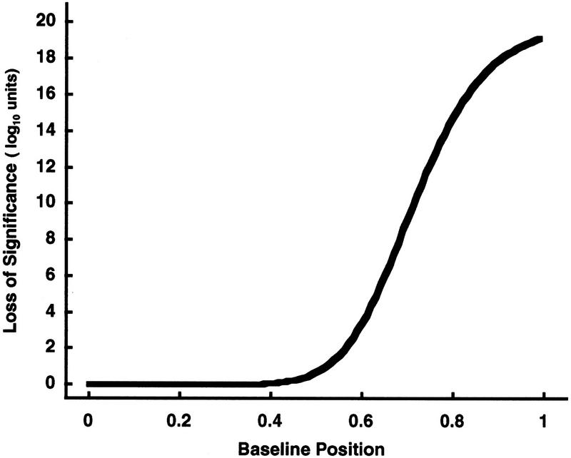
The effects of the baseline adjustment factor λ on the traditional Dixon significances are shown in columns 5–7. In Figure 7 the Δlog₁₀(sp) is plotted as a continuous function of baseline encroaching toward the maximum allowed intensity. As desired for baseline adjustments of significance, the erosion in statistical confidence reflected by the loss of significance probability Δlog₁₀(sp) becomes substantial when the baseline encroaches upon the maximum allowed intensity (i.e., 1).

Figure 7.

Erosion of confidence increases as the baseline position increases toward the maximum. The number of samples (n = 22), the maximum intensity (x_n = 1), and the traditional Dixon significance probability [log₁₀(sp) = −20) are kept fixed throughout this example as in Fig. 5. The resulting erosion of confidence, i.e., the loss of statistical significance Δlog₁₀(sp) from the traditional Dixon value, is plotted continuously as the baseline increases toward the allowed maximum intensity (see also Table 1).

An important general principle is illustrated by these examples: Though the traditional Dixon statistical significance probability can remain extremely strong (e.g., 10⁻²⁰) even as the dynamic range of the data is compressed ever smaller (represented here by the baseline coming ever closer to an allowed maximum), a baseline compression adjusted significance probability can nonetheless reflect the erosions of statistical significance that should occur in data whose dynamic range is substantially compressed.

Whereas there is no intrinsic method to determine how much outlier statistical significance probability ought to be attenuated, scientific judgment concerning data accuracy, the resolving power of intensity measurement techniques, and the dynamic range of intensity data can be used to design significance adjustment functions.

Step 6—Decision Function

Design a decision function d, 0 ⩽ d ⩽ 1, as discussed qualitatively in step 6 of the Algorithm section. d near 0 is interpreted as very weak overall confidence, whereas d near 1 is very strong overall confidence in selective expression detection.

To construct d, we need to introduce normalized, transformed versions of the gap (equation 3) and significance probability (equation 11) that are contained in [0,1]. Those gaps which meet a minimum gap threshold (g_thresh) are rescaled linearly between a minimum gap threshold g_thresh and the maximum possible gap of 1 (equations 1b and 3):

13

Analogously, linearly transform the baseline compression adjusted significance log₁₀(sp_adjusted) (equation 11) between the weakest-to-strongest statistical significances that one is willing to accept, that is, between log₁₀(sp)_thresh and log₁₀(sp)_∞, respectively. The lower bound log₁₀(sp)_∞ is the statistical significance beyond which stronger significance is essentially inconsequential. Denoting s, (0 ⩽ s ⩽ 1), as this transformation gives:

The choices of gap and significance probability thresholds are up to the user. To be conservative, we often choose log₁₀(sp)_thresh = −5 instead of the more conventional −3. For log₁₀(sp)_∞ we have found that −20 is a reasonable choice allowing the significance probability a dynamic range of 10¹⁵.

d is designed to capture the biological notions of confidence, which are summarized in Table 2. Either a log₁₀(sp_adjusted) or a gap weaker than their respective thresholds (equations 13 and 14) is not selective expression, and d is immediately 0 in such cases. In Table 1, d is moderate even when s is strong if, in conjunction, g is weak. This reflects an erosion of confidence that should occur when a gap is near the intensity measurement’s resolving power, as discussed in the Step 5 Details. Also, note that d is strong when g is strong even if s is weak. A strong gap confers strong confidence in this case because even a weak s is still a significance probability that is stronger than a rather conservative threshold (e.g., log₁₀(sp)_thresh = −5). Thus, there is no a priori requirement that d be symmetrical with respect to s and g. We prefer in practice an asymmetry that gives more importance to large gap values as long as log₁₀(sp_adjusted) is stronger than a conservative threshold.

Table 2.

Selective Expression Confidences According to a Decision Function

		Scaled gap ga
		weak (g ≈ 0)	strong (g ≈ 1)
Scaled signal  probability, sb	weak (s ≈ 0)	weak (d ≈ 0)	strong (d ≈ 1)
strong (s ≈1)	moderate (d ≈1)	strong (d ≈1)

See Step 6 of the Details section for a discussion; equation 15 is a representative function for d. 

^aEquation 13. 

^bEquation 14. 

A decision function that incorporates these principles is

15

where α > 0, β > 0, γ > 0, and δ (0 < δ < 1) are independent parameters chosen empirically, and φ = (α + β + γ)⁻¹. Observe that the term in brackets amounts to a numerical version of a logical and of three terms, the third term of which amounts to a numerical logical or of two terms blended in a proportion controlled by δ. The function d is contained in [0,1].

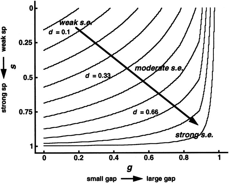
Typically, we choose α = β = γ = 1.5 and δ = 0.3. Figure 8 shows this decision function d plotted as a series of constant d contours in (g,s) space. Calibrating ranges of δ contours against weak to strong archetypes of the user’s choosing is up to the user. Though there is no intrinsic method for setting break points between weak, moderate, and strong confidences, in practice we take these to be 1/3 and 2/3, respectively.

Figure 8.

Decision function for selective expression of overall confidence. The decision function [d(g,s), equation 15] is plotted as constant d contours in the space of (g,s) coordinates, each ≥0 and ⩽1. (g,s) Respective linear transformations of gap and baseline adjusted log₁₀(sp) between the weak thresholds and strong limits (equations 13 and 14). Overall confidence of a selective expression is assessed by the value of the decision function, weak being associated with d near 0 and strong associated with d near 1. Typically, we assign overall confidences as weak when 0 ⩽ d < 0.33, moderate when 0.33 ⩽ d < 0.66, and strong when 0.66 ⩽ d ⩽1.

It is noted that the decision function is somewhat analogous in character to document retrieval similarity functions as defined by Salton for information retrieval from databases (Salton 1989). These similarity functions are highly nonlinear functions of weighted combinations of Boolean-like query vectors and document information content feature vectors. As in the decision function, each feature is a scalar between 0 and 1, and the function returns a scalar between 0 and 1. Retrieval similarity functions provide a means by which retrieved documents can be ranked in order of similarity to a given multicomponent query. Analogously, the decision function provides a means by which intensity patterns can be ranked in order of confidence in their being selective expression.

Application of the Selective Expression Algorithm

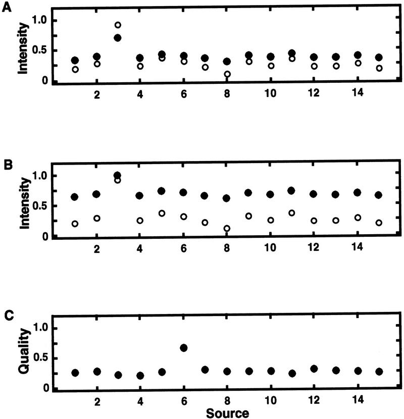
Selective expression detection results will be illustrated through a set of examples. The examples are shown in Figure 9, with source qualities and corresponding intensities in Table 3, and computed numerical results summarized in Table 4. Though these intensity and source quality data are synthetic, they are representative of real examples derived from a large database of gene abundances and library qualities.

Figure 9.

Examples of synthetic, yet realistic, intensity (abundances) vs. source (library) data for genes. (A) Example 2 (●) and example 1 (○) are compared; (B) example 3 (●) vs. example 1 (○); (C) source qualities corresponding to the intensities. In A and B, the putative selective expression occurs in the third source. The numerical values of the data along with the computed baseline estimate x̂_baseline and separation ratios τ are presented in Table 3. The accompanying selective expression algorithm summarized calculations are in Table 4.

Table 3.

Examples: Synthetic, yet Realistic, Intensity (Abundance) and Source (Library) Quality Data for Genes (Assemblies)

Source	Quality	Example
1	2	3
1	0.26	0.19	0.35	0.64
2	0.27	0.29	0.39	0.68
3	0.22	0.92	0.71	1.00
4	0.20	0.24	0.37	0.66
5	0.26	0.37	0.43	0.72
6	0.65	0.31	0.40	0.69
7	0.29	0.21	0.35	0.64
8	0.26	0.10	0.30	0.59
9	0.26	0.30	0.40	0.69
10	0.26	0.23	0.37	0.65
11	0.21	0.35	0.43	0.72
12	0.28	0.22	0.36	0.65
13	0.26	0.21	0.36	0.64
14	0.25	0.26	0.38	0.67
15	0.22	0.17	0.34	0.63
x̂baselinea		0.25	0.38	0.66
gapb		0.55	0.28	0.28
τc		0.67	0.68	0.68
τadjustedd		0.67	0.68	0.58

See Fig. 9 for the corresponding intensity vs. source plots. We set f_max = 1 in these examples. See Results for the baseline estimate equation. See Table 4 for the accompanying algorithmic calculations summarized. 

^aEquation 10 with k = n − 1. 

^bEquation 3. 

^cEquation 4. 

^dEquation 8. 

Table 4.

Examples: The Selective Expression Algorithm Applied to Synthetic, yet Realistic, Data

Example	Baseline adjusted	λa	gapb	τc	log10(sp)d	de	Comments
1a	no		0.55	0.67	−6.26	0.33	reference example
1b	yes	1.00	0.55	0.67	−6.27	0.33	same as 1a; λ has no effectf
2a	no		0.28	0.68	−6.26	0.24	d different from 1a due to  gap only
2b	yes	0.99	0.28	0.68	−6.28	0.24	d different from 1a due to  gap; λ has no effectf
3a	no		0.28	0.68	−6.26	0.24	d different from 1a due to  gap only
3b	yes	0.87	0.28	0.58	−4.90	0.00	d different from 1a due to  λ−adjusted log10(sp) > −5,  hence d = 0g

The example identification (1, 2, or 3) corresponds to Fig. 9; whether a baseline compression adjustment was omitted (a) or used (b) in the discordancy computation (equation 6 or 11). The intensities and source quality weights are from Table 3. 

^aEquation 9. 

^bEquation 3. 

^cEquation 4. 

^dEquation 6 or 11. 

^eEquation 15. Equation 9 sigmoidal parameters are b = 10 and c = 0.8. The parameter values in the decision function d (equations 13–15) are α = β = γ = 1.5, δ = 0.3, g_thresh = 0.25, log₁₀(sp)_thresh = −5, and log₁₀(sp)_∞ = −20. 

^fλ has no effect, as the baseline (i.e., ∼0.3, Table 3) is distant from the maximum allowed intensity (i.e., 1). 

^gλ has non-negligible effect, as the baseline is near (i.e., 0.67, Table 3) the maximum intensity. 

To convey the effects of various components of the algorithm, each example of Figure 9 and Table 3 is constructed deliberately to have very similar qualitative patterns of intensity versus source. Yet, the examples are different in overall confidence of selective expression. Each example has the same source set (size n = 15) and, moreover, exactly the same separation ratio (τ = 0.67) before any adjustments are made for baselines. Hence, these examples have by design exactly the same traditional Dixon statistical significance probability before baseline compression adjustment.

Table 4 shows the effects of the algorithm’s components. For example, the effects of adjusting the statistical significance probability for baseline can be seen by comparing each example after adjustment for baseline (case b) against its respective case unadjusted for baseline (case a). Example 3 is the only case in which statistical significance probability is changed nonnegligibly by baseline adjustment. This can be appreciated by observing in case 3b the effects of baseline on λ, hence on τ, when compared against the reference case 1a.

Examples 2 and 3, however, have markedly smaller gaps than does example 1. These diminutive gaps are responsible for the respective decision function values being much smaller even though the discordancy statistical significance probabilities (with or without baseline adjustments) are not changed much. The exception is case 3a, which has an ample loss of significance probability due to baseline adjustment. Though the 3b gap is the same as 3a, 3b’s decision function is zero because baseline adjustment of its significance probability has resulted in its log₁₀(sp_adjusted) not meeting the minimum statistical significance criterion of log₁₀(sp)_thresh = −5.

Taken together, these examples illustrate how qualitatively similar intensity versus source patterns can have different overall confidences of selective expression determination. The decision function values depend on the baseline of the data and the size of the gap, even when the expression patterns have essentially identical unadjusted discordancy significance probabilities. By analyzing these examples, it can be seen how the qualitatively stronger overall confidence of selective expression of example 1 as compared to examples 2 and 3 (which is informally conveyed in Fig. 9) is quantitated through the decision function.

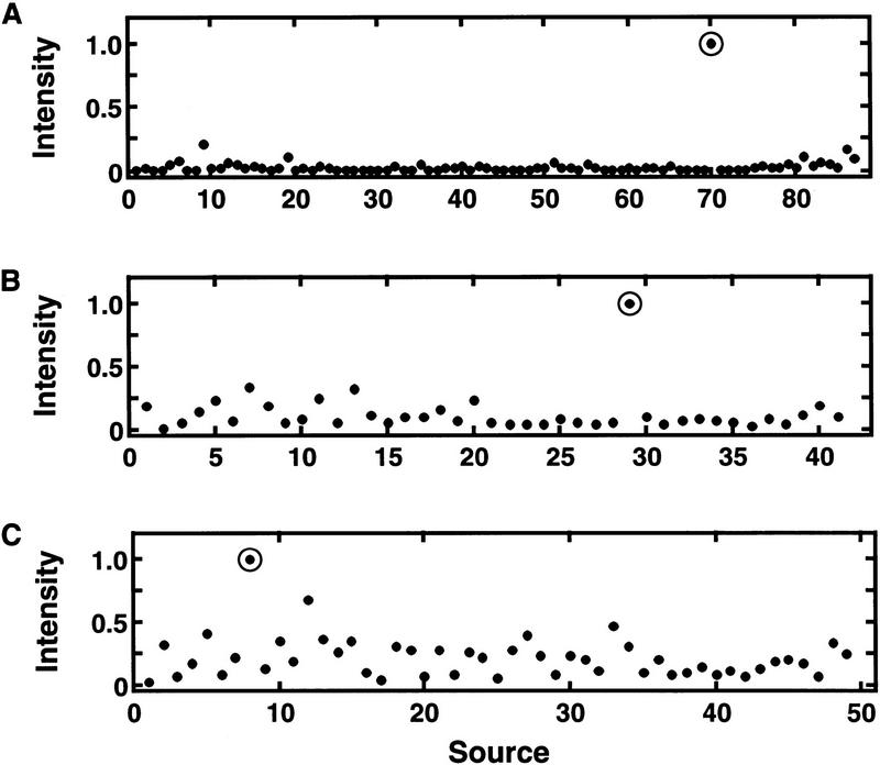
Also, to convey the appearances of stereotypical selective expression patterns in real gene expression data, intensity versus source plots of some actual examples of algorithmically detected extremely strong, strong, and weak overall confidence selective gene expression are shown in Figure 10. Calculations corresponding to these examples are shown in Table 5. In these particular examples, baseline adjustment has no effect because the baselines are well below 0.5 of the maximum intensity. Hence, the discordancy statistical significance probabilities are the same as the unadjusted ones.

Figure 10.

Stereotypical examples of selective expression in real abundance data as detected by the algorithm. Intensities (abundance) vs. source (library) for three assemblies from a real database of sources and assembly abundances are plotted. (A) An extremely strong overall confidence of selective expression (decision function d = 1.0); (B) strong overall confidence of selective expression (d = 0.75); (C) weak overall confidence of selective expression (d = 0.31). Calculations from the algorithm are summarized in Table 5.

Table 5.

Stereotypical Examples of Selective Expression in Real Data as Detected by the Algorithm

Example	No.	x̂baselinea	λb	gapc	τd	log10(spadjusted)e	df	Overall confidence in s.e.
A	87	0.03	1.0	0.78	0.78	−56.0	1.0	very strong
B	41	0.10	1.0	0.66	0.67	−18.8	0.7	strong
C	47	0.20	1.0	0.34	0.34	−8.5	0.3	weak

See Fig. 10 for corresponding intensity vs. source plots. See Results for discussion. The equations’ parameter values are the same as those used in Table 4. 

^aEquation 10 with k = n − 1. 

^bEquation 9. 

^cEquation 3. 

^dEquation 8. 

^eEquation 11. 

^fEquation 15. 

From Table 5, the τ are decreasing from example A to C, with the larger decrease being from example B to C. That the statistical significance probabilities decrease so dramatically with this series of τ values is because of the considerable size of the n involved. The marked difference in log₁₀(sp) between A and B is caused much more by the difference in n than in τ. However, the substantial difference in log₁₀(sp) between B and C is caused by the difference in τ more than the difference in n. These differences are not surprising given the nonlinear dependence of log₁₀(sp) on τ in equation 6 (visualized in Figs. 3 and 4). Clearly, A is an extremely strong overall confidence selective expression determination, as can be recognized visually in Figure 10 and quantitatively in Table 5. That the d for C is half that for B is due to both the gap and the log₁₀(sp) in combination being weaker in C than B.

To understand the data it can be useful to dissect the various contributions to the decision function as done above. However, the real power of the decision function is its utility in qualitatively ranking selective expression patterns in large-scale data in a way that is not only easily automated, but objective and consistent.

To convey the application of the algorithm to large-scale data, results from a large database of assemblies are depicted in Figure 11 (see equations 13–15). Each assembly that is identified by the algorithm as being selectively expressed is plotted (bubble symbol) according to its transformed gap (equation 13) and statistical significance (equation 14) values. Note the relatively small number of high confidence selectively expressed assemblies (d > 0.66). The decision function values provide an objective means by which assemblies can be rank ordered by their selective expression confidence. This is useful in setting priorities for further analysis or experimentation. Moreover, by focusing attention on assemblies with the strongest selective expression confidences, follow-up efforts may be more efficiently concentrated on a relatively small subset.

Figure 11.

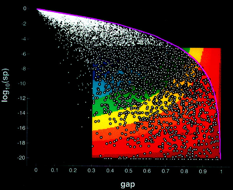
Selective expression in large-scale data. Results of the algorithm applied to a large database of assembly expression data are indicated. Each assembly is plotted as a point according to its gap (equation 3) and statistical significance log (sp_adjusted) (equation 11). Those assemblies identified by the algorithm as being selectively expressed are plotted using bubble symbols. When these assemblies’ gap and log(sp_adjusted) are transformed using equations 13 and 14, respectively, the resulting (g,s) fall within the (g,s)-unit square; hence, these assemblies are selectively expressed. The area enclosed by the rectangular region bounded by g_thresh ⩽ gap ⩽ 1, g_thresh = 0.3, on the abscissa and by −20 ⩽ log₁₀(sp_adjusted) ⩽ −5 on the ordinate is colored using a conventional spectrum. The coloring is according to the confidence of selective expression, i.e., the strength of the decision function d(g,s) (equation 15) corresponding to [gap, log(sp)] within the rectangle. The confidence (d) color coding is blue for low, yellow–orange for moderate, and red for high. The red region directs the eye to the assemblies with the strongest confidence of selective expression. However, those assemblies identified by the algorithm as being not selectively expressed, i.e., not meeting the minimum gap criterion or not meeting the minimum statistical significance criterion [log₁₀(sp)_thresh = −5], are plotted as solid dots in [gap,log(sp)] coordinates. These gap and log(sp_adjusted), when transformed by equations 13 and 14, fall outside the (g,s)-unit square, hence, to the left or above the colored rectangular region in gap,log(sp)]-space. The weakest possible statistical significance as a function of gap is the curve plotted in magenta. This upper-bound curve represents log(sp) (equation 6) when the number of intensities equals the minimum number of sources criterion, namely n = 10, where x_n − x₁ is as large as possible, i.e., 1; hence, τ = gap (equation 4).

DISCUSSION

We have shown that selective expression can be identified robustly by the presented algorithm. The algorithm uniquely combines a statistical test of discordancy, source reliability weighted adjustments for baseline levels of the intensities, and adjustments for the separation of the largest from the next-to-largest intensity (gap) to give an overall assessment of confidence in selective expression detection. The algorithm achieves this by combining the various ingredients—statistical discordancy, baseline compression adjustment, and gap—into a decision function that takes into account all these in a consistent and reliable manner. We have also argued that any one or two of these ingredients alone are insufficient for reliable selective expression determination. It is the decision function and its ability to assess the confidence of the prediction that is the true strength of the algorithm. Incorporating biological knowledge into the decision function strengthens the overall algorithm. It minimizes the risk of statistical artifacts causing a false-positive determination.

The algorithm is generally applicable to expression data whether derived from DNA, RNA, or proteomics. Though the algorithm was developed originally for analyses of gene expression, it is in fact rather general, being applicable to many kinds of intensity data associated with sources and, preferably, for which reliabilities of the sources can be assessed. Moreover, the algorithm is indifferent as to whether the intensities are experimental or computationally derived. The algorithm is well-suited to be used with large databases and large numbers of sources. The algorithm’s work is linear in both the number of database entries and in the number of sources considered.

The algorithm has been successfully implemented to analyze large databases of gene abundances routinely. Computationally identified strong selective expression is a relatively rare phenomenon among the gene abundance databases being analyzed. Yet, it is frequent enough to suggest plentiful opportunities for additional analysis. A number of biologically and pharmacologically interesting selectively expressed genes have been identified for further confirmatory experimentation.

There are several areas in which extensions can be made. The first is to include consideration of knowledge of uncertainties in individual intensities. This will become extremely important in considering values close to the detection limit or if the signal-to-noise ratio is low. The second extension is to calculate the sensitivities of the decision function to slight changes in τ or gap. Errors in the expression data lead to uncertainties in both τ and gap; these uncertainties could be propagated into the decision function calculation.

REFERENCES

- Adams MD. Expressed sequence tags as tools for physiology and genomics. In: Adams MD, Fields C, Venter JC, editors. Automated DNA sequencing and analysis. London, UK: Academic Press; 1994. pp. 71–80. [Google Scholar]
- Adams MD, Fields C, Venter JC. Automated DNA sequencing and analysis. London, UK: Academic Press; 1994. [DOI] [PubMed] [Google Scholar]
- Anderson L, Seilhamer J. A comparison of selected mRNA and protein abundances in human liver. Electrophoresis. 1997;18:533–537. doi: 10.1002/elps.1150180333. [DOI] [PubMed] [Google Scholar]
- Anderson NL, Hofmann J-P, Gemmell A, Taylor J. Global approaches to quantitative analysis of gene-expression patterns observed by two-dimensional gel electrophoresis. Clin Chem. 1984;30:2031–2036. [PubMed] [Google Scholar]
- Audic S, Claverie J-M. The significance of digital gene expression profiles. Gen Res. 1997;7:986–995. doi: 10.1101/gr.7.10.986. [DOI] [PubMed] [Google Scholar]
- Barnett V, Lewis T. Outliers in statistical data. Chichester, UK: Wiley; 1978a. [Google Scholar]
- ————— . Outliers in statistical data. Chichester, UK: Wiley; 1978b. p. 4. [Google Scholar]
- ————— . Outliers in statistical data. Chichester, UK: Wiley; 1978c. p. 23. [Google Scholar]
- Bossard MJ, Tomaszek TA, Thompson SK, Amegadzie BY, Hanning CR, Jones C, Kurdyla JT, McNulty DE, Gowen M, Levy MA. Proteolytic activity of human osteoclast cathepsin K—expression, purification, activation, and substrate identification. J Biol Chem. 1996;271:12517–12524. doi: 10.1074/jbc.271.21.12517. [DOI] [PubMed] [Google Scholar]
- Britten RJ, Kohn DE. Repeated sequences in DNA. Science. 1968;161:529–540. doi: 10.1126/science.161.3841.529. [DOI] [PubMed] [Google Scholar]
- Bunge J, Fitzpatrick M. Estimating the number of species: A review. J Am Stat Assoc. 1993;88:364–373. [Google Scholar]
- Burks C, Engle ML, Forrest S, Parsons RJ, Soderlund CA, Stolorz PE. Stochastic optimization tools for genomic sequence assembly. In: Adams MD, Fields C, Venter JC, editors. Automated DNA sequencing and analysis. London, UK: Academic Press; 1994. pp. 250–259. [Google Scholar]
- Drake FH, Dodds RA, James IE, Connor JR, Debouck C, Richardson S, Lee-Rykaczewski E, Coleman L, Rieman D, Barthlow R, et al. Cathepsin K, but not cathepsins B, L, or S, is abundantly expressed in human osteoclasts. J Biol Chem. 1996;271:12511–12516. doi: 10.1074/jbc.271.21.12511. [DOI] [PubMed] [Google Scholar]
- Galau GA, Klein WH, Britten RJ, Davidson EH. Significance of rare mRNA sequences in liver. Arch Biochem Biophys. 1977;179:584–599. doi: 10.1016/0003-9861(77)90147-3. [DOI] [PubMed] [Google Scholar]
- Grubbs FE. Procedures for detecting outlying observations in samples. Technometrics. 1969;11:1–21. [Google Scholar]
- Gumbel EJ. Statistics of extremes. New York, NY: Columbia University Press; 1958. [Google Scholar]
- Hames BD, Higgins SJ. Nucleic acid hybridisation—A practical approach. Oxford, UK: IRL Press Limited; 1985. [Google Scholar]
- Hawkins DM. Identification of outliers. London, UK: Chapman & Hall; 1980. [Google Scholar]
- Herbert BR, Sanchex J-C, Bini L. Two-dimensional electrophoresis: The state of the art and future directions. In: Wilkins MR, Williams KL, Appel RD, Hochstrasser DF, editors. Proteome research: New frontiers in functional genomics. Berlin, Germany: Springer-Verlag; 1997. pp. 13–33. [Google Scholar]
- Lewin B. Genes V. New York, NY: Oxford University; 1994. [Google Scholar]
- Lewins WA, Joanes DN. Bayesian estimation of the number of species. Biometrics. 1984;40:323–328. [Google Scholar]
- Lodish H, Baltimore D, Berk A, Zipursky SL, Matsudaira P, Darnell J. Molecular cell biology. 3rd ed. New York, NY: Scientific American Books/W.H. Freeman and Co.; 1995. [Google Scholar]
- Myers EW. Advances in sequence assembly. In: Adams MD, Fields C, Venter JC, editors. Automated DNA sequencing and analysis. London, UK: Academic Press; 1994. pp. 231–248. [Google Scholar]
- Patanjali S, Parimoo S, Weissman SM. Construction of a uniform-abundance (normalized) cDNA library. Proc Natl Acad Sci. 1991;88:1943–1947. doi: 10.1073/pnas.88.5.1943. [DOI] [PMC free article] [PubMed] [Google Scholar]
- Poschel T, Ebeling W, Rose H. Guessing probability distributions from small samples. J Stat Phys. 1995;80:1443–1452. [Google Scholar]
- Robbins HE. Estimating the total probability of the unobserved outcomes of an experiment. Ann Math Stat. 1968;39:256–257. [Google Scholar]
- Sachs L. Applied statistics—A handbook of techniques. 2nd ed. New York, NY: Springer-Verlag; 1982. [Google Scholar]
- Salton G. Automatic text processing: The transformation, analysis, and retrieval of information by computer. Reading, MA: Addison-Wesley; 1989. [Google Scholar]
- Singer M, Berg P. Genes & genomes. Mill Valley, CA: University Science Books; 1991. [Google Scholar]
- Wilkins MR, Williams KL, Appel RD, Hochstrasser DF. Proteome research: New frontiers in functional genomics. Berlin, Germany: Springer-Verlag; 1997. [Google Scholar]
- Zhao B, Janson CA, Amegadzie BY, D’Alessio K, Griffin C, Hanning CR, Jones C, Kurdyla J, McQueney M, Qui X, et al. Crystal structure of human osteoclast cathepsin K complex with E-64. Nat Struct Biol. 1997;4:109–111. doi: 10.1038/nsb0297-109. [DOI] [PubMed] [Google Scholar]