Abstract
This paper examines how control engineering and risk management techniques can be applied in the field of behavioral health through their use in the design and implementation of adaptive behavioral interventions. Adaptive interventions are gaining increasing acceptance as a means to improve prevention and treatment of chronic, relapsing disorders, such as abuse of alcohol, tobacco, and other drugs, mental illness, and obesity. A risk-based Model Predictive Control (MPC) algorithm is developed for a hypothetical intervention inspired by Fast Track, a real-life program whose long-term goal is the prevention of conduct disorders in at-risk children. The MPC-based algorithm decides on the appropriate frequency of counselor home visits, mentoring sessions, and the availability of after-school recreation activities by relying on a model that includes identifiable risks, their costs, and the cost/benefit assessment of mitigating actions. MPC is particularly suited for the problem because of its constraint-handling capabilities, and its ability to scale to interventions involving multiple tailoring variables. By systematically accounting for risks and adapting treatment components over time, an MPC approach as described in this paper can increase intervention effectiveness and adherence while reducing waste, resulting in advantages over conventional fixed treatment. A series of simulations are conducted under varying conditions to demonstrate the effectiveness of the algorithm.
Index Terms: Risk Analysis, Predictive Control, Process Control, Adaptive Interventions, Behavioral Health
INTRODUCTION
Behavioral interventions play a prominent role in the prevention and treatment of a wide number of public health disorders, among these abuse of alcohol, tobacco, and other drugs, mental illness, and obesity. Traditional fixed interventions provide the same dosages of prevention or treatment components to all program participants, without taking into account any individual features. Recent efforts in the fields of medicine and behavioral health have suggested that tailoring treatment to the specific needs of an individual participant may enable delivery of interventions with greater degrees of efficacy and adherence, and less waste [1]; this is the motivating principle for adaptive interventions (also known as contingency management, stepped care programs, and case management, [2]). In an adaptive intervention, different dosages of prevention or treatment components are assigned to different individuals across time, with dosage varying in response to the needs of the individual. Adaptive interventions are time-varying when the dosage is revised repeatedly throughout the intervention. Time-varying adaptive interventions are particularly well-suited for addressing chronic disorders that are relapsing in nature; contributions of adaptive interventions for the treatment of hypertension [3], depression [4], substance abuse [5], [6], [7], [8], Alzheimer’s disease [9] and infectious diseases [10] have been reported.
The work in [2] presents a conceptual framework for adaptive interventions and discusses principles that underlie the design and evaluation of such interventions. This work serves as the basis for the analysis in [11], which demonstrates that adaptive interventions are feedback control systems, and as such will benefit from a control-theoretic approach. The objective of this paper is to extend the work reported in [11] by incorporating a risk-management perspective within a Model Predictive Control (MPC) framework. The proposed control-oriented framework replaces the “IF-THEN” and PID control-based decision rules presented in [11] with a formal framework that incorporates risks based on Model Predictive Control.
Risk management is a relatively new perspective that was first applied to natural disasters [12], but in the last decade has been extended to the fields of project management and financial policies, in which it is generating a growing interest [13], [14]. Risk management can be summarized as the identification of risks, their ranking or prioritization, the resolution of those deemed significant and their monitoring through their applicable life. Methods and disciplines that address risk management are becoming more highly accepted by companies, as those organizations which better understand the nature of risks (and can thus manage them more effectively) can not only avoid unforeseen disasters, but can also operate with tighter margins and less contingency [15].
In this paper we illustrate a risk-based, control-oriented framework for decision-making in adaptive interventions by means of a hypothetical yet meaningful simulated intervention. By using a risk-based approach, information about additional factors that may affect the evolution of the participant state during the intervention period can be considered. The controller incorporates additional manipulated variables which represent mitigation actions that can be undertaken in order to reduce risk exposure. These actions can either increase or decrease the treatment dosage, or result in a switch to other treatment options if risks take place. MPC, the control methodology that executes these decisions, has been widely used in applications as diverse as manufacturing [16], economic systems [17] and medicine [18]. Among the reasons for use of MPC include the ease with which it handles constraints, its ability to naturally incorporate a model representing the problem phenomena, and its ready extension to the multivariable case.
The hypothetical adaptive intervention considered in this paper is patterned after the Fast Track program [19], [20], [21]. The long-term objective of this program is to prevent conduct disorder in at-risk children. Whereas the core intervention components in Fast Track were fixed, a series of components were delivered adaptively. We focus in this paper on the frequency of home-based counseling visits, which were assigned to each family during the course of the intervention depending upon the level of parental functioning. In the formulation of the Case Study we rely on risks identified by the Social Development Research Group (SDRG) at the University of Washington [22], [23], an organization focused on prevention and treatment programs geared for youth.
This paper is organized as follows. Section II describes a hypothetical time-varying adaptive intervention inspired by Fast Track. The section presents a dynamic model representation of this process and how the intervention can be conceptualized as a closed-loop dynamical system. Section III presents the proposed risk modeling approach, while Section IV describes the risk-based optimal control algorithm based on MPC. A case study is presented and discussed in Section V where a series of nominal and Monte Carlo simulations are presented to show the benefits of the method. Some concluding remarks are highlighted in Section VI.
II. ADAPTIVE BEHAVIORAL INTERVENTIONS AS CLOSED-LOOP DYNAMICAL SYSTEMS
As a representative example of a time-varying adaptive intervention we examine the Fast Track program developed by the Conduct Problems Prevention Research Group (CPPRG) [19], [20], [21]. Fast Track was a multi-year, multi-component program designed to prevent conduct disorder in at-risk children. Youth showing conduct disorder are at increased risk for incarceration, injury, depression, substance abuse, and death by homicide or suicide. In Fast Track, some intervention components were delivered universally to all participants, while other specialized components were delivered adaptively. In this paper we base our hypothetical examples on the family counseling component of Fast Track, which was provided to families on the basis of parental functioning.
There are several possible levels of intensity, or doses, of family counseling. The objective of our hypothetical intervention is to vary the doses of family counseling depending on the needs of the family, in order to avoid providing an insufficient amount of counseling for very troubled families, or wasting counseling resources on families that may not need them or may be stigmatized by excessive counseling. The decision about which dose of counseling to offer each family is based primarily on the family’s level of functioning, assessed by a family functioning questionnaire completed by the parents. The score on the family functioning questionnaire is referred to in [2] as the tailoring variable, because it is used to determine the particular level of treatment provided to the individual family. Another factor which may affect the value of the tailoring variable is the judgment of a clinician familiar with the family’s case. Based on the questionnaire and the clinician’s assessment, family functioning is determined to fall in one of the following categories: very poor, poor, near threshold, or at/above threshold. A corresponding decision rule that can be applied is as follows: families with very poor functioning are given weekly counseling; families with poor functioning are given biweekly counseling; families with near threshold functioning are given monthly counseling; and families at or above threshold are given no counseling. Family functioning is reassessed at a review interval of three months, at which time the intervention dosage may change. This goes on for three years, with twelve opportunities for a dose of family counseling to be assigned.
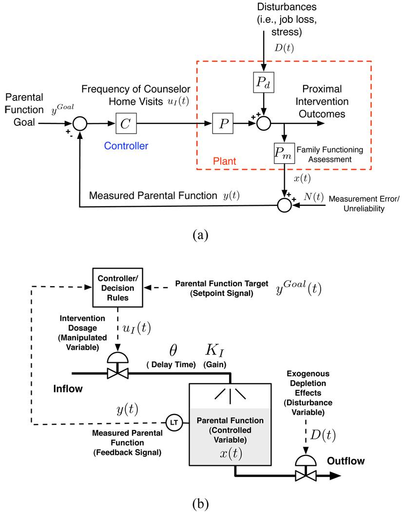
This adaptive intervention has previously been studied from a control perspective in [11]. In a control engineering context, the frequency of counseling visits (the intervention dosage) is the manipulated variable, while parental function is the state variable. Measured parental function (performed at quarterly intervals) is the controlled variable and serves as the tailoring variable for the intervention. Decision rules correspond to controllers that take values of the tailoring variable and correspondingly assign intervention dosages. Disturbances represent exogeneous factors that influence parental function during the course of an intervention. While some disturbances can be considered as beneficial in character (e.g., new job, pay raise, or vacation time), we will focus in this paper on disturbances that negatively affect parental function (e.g., job loss, stress, or illness). Disturbances were described generically in [11], but these will be defined more explicitly in the form of risks in Section V of the present paper. Figure 1(a) depicts a block diagram corresponding to the representation of an adaptive intervention as a feedback control system (as discussed in [11]) and Figure 1(b) shows the corresponding fluid analogy.
Fig. 1.
Block-diagram representation (a) and corresponding fluid analogy (b) of a hypothetical family counseling-home visits adaptive intervention patterned after the Fast Track program.
An important consideration in applying a control engineering perspective to this problem is how to model the open-loop dynamics of the closed-loop system depicted in Figure 1(a). In this paper we rely on the work in [11] to apply a fluid analogy to describe the “open-loop” dynamics of the adaptive intervention:
| (1) |
| (2) |
| (3) |
where uI(t) is the frequency of counselor home visits and represents the manipulated variable, x(t) is the parental function and represents the tailoring or controlled variable for the intervention, D(t) is the disturbance or depletion signal, considered as a collective effect of multiple events, N(t) is the measurement noise, KI is the intervention gain, and θ represents the time delay between the intervention and its actual effect on parental function. The model according to Equations 1–3 corresponds to conservation of mass in a production-inventory system, which denotes a parallel between this problem and inventory management in supply chains. In the latter problem, fluid analogies and control-oriented approaches have led to sound, practical solutions, despite conditions of stochasticity and uncertainty [24], [25].
The design of a time-varying adaptive intervention is a process that may involve considerable uncertainty. Uncertainty may stem in part from the nature of the measurements, which may rely on clinical staff judgement and error-prone assessment instruments such as questionnaires. There may also be variations in response between individuals (e.g., the same intervention dosage may provide different results in two different individuals) and variation in an individual’s response when examined at different times. The response of the system will depend heavily on external factors. The following section describes how a risk management approach provides a means to model the effect of the unknown factors.
III. RISK MANAGEMENT IN ADAPTIVE INTERVENTIONS
Many studies have put forth efforts to identify risk factors associated with behavioral health. One example is [26], where a telephone-based intervention appears to be an effective form of step-down treatment for participants with alcohol and cocaine dependence who complete an initial stabilization treatment. Prior to providing the intervention to a participant, individual risk factors are analyzed to determine its suitability.
External risk factors may be considered as disturbances in the sense that they can change the expected outcomes. If these disturbances are not taken into account, decision making on the control variable may not be as effective. Risk management is aimed at making decisions in systems where limited knowledge about the process, system complexity and the presence of uncertainties at critical points in time have a decisive role. In this paper, particular disturbances that can be identified a priori will be referred to as risks. Risk modeling as applied to an adaptive intervention is described in the ensuing subsections.
A. Risk Modeling
In this work, the term risk is defined as an event that could take place and cause impacts to a participant seeking treatment. Therefore, the first step in applying risk management is to carry out an identification of the possible risks (Ri). We define R = {R1, …, Rm} as the set of identified risks for a specific participant. Each risk is characterized by a probability of occurrence in each time period (pi(t)) and some impacts (Ii) which may affect the individual by decreasing or increasing the efficiency of the interventions, if the risk were to occur and no mitigating actions are taken.
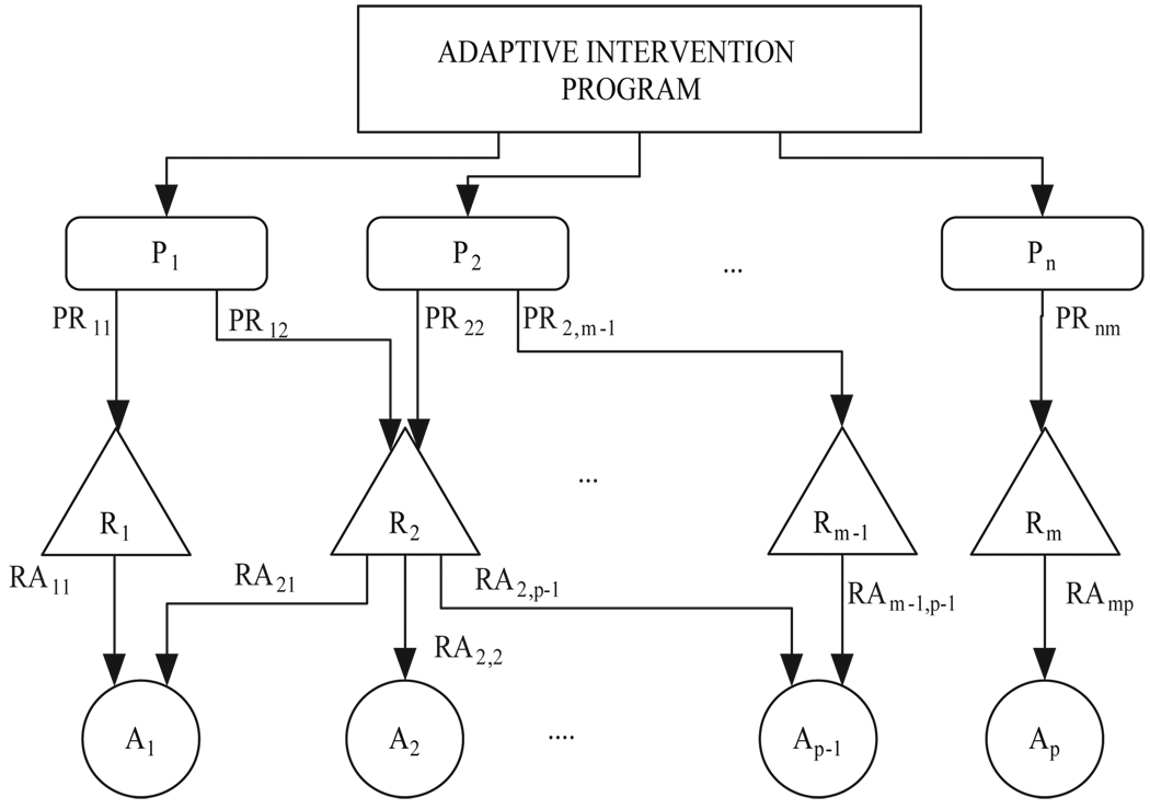
Once risk identification has been performed, the next step to undertake is the design of a strategic mitigation plan from a clinical point of view. This makes possible the impact reduction of the identified risks and hence, the adaptation of the treatment for each individual. In this way, each risk can be associated with a set of actions (Ai) that could mitigate these risks. Figure 2 shows an example of a Risk-Based Structure (RBS) that illustrates the relationship between risks and actions in a possible strategic plan.
Fig. 2.
Illustration of a Risk-Based Structure (RBS) for participants P1, P2, …, Pn receiving an intervention
It can be observed that a participant (Pi) may be associated with some specific risks (i.e., participant 1 is susceptible to risks R1 and R2); a risk can be mitigated by different actions. In Figure 2 for example, R2 is mitigated by A1, A2 and Ap−1. One action may mitigate different risks; note in Fig. 2 how A1 mitigates R1 and R2. Mitigating actions will reduce the initial impact of a risk, but usually, the system will incur additional costs as a result. Even if the impact is stochastic in nature (i.e., assessed only if the risk actually occurs), costs associated with mitigating actions will be incurred regardless. There is an arc from participant Pj to risk Ri labeled by PRji if participant Pj incurs risk Ri; PRji = 0 if participant Pj does not incur risk Ri. On the other hand, there is an arc from risk Ri to action Ak, labeled by RAik if Ri is mitigated by action Ak; RAik = 0 if action Ak does not mitigate risk Ri.
We assume the mitigation action set as A = {A1, …, Ap} with p representing the number of mitigation actions. Formally, each mitigation action is described by a set of three elements:
| (4) |
where the decision variable for the action (Ai) is denoted by uFi· fi(uFi) : ℜ → ℜ is a function that determines the risk impact reduction as a function of uF in each unit time; thus, fi is the reduction of the initial impact when the action (Ai) is applied. Actions that are chosen to mitigate risks may have an associated cost of execution; this feature is modelled by defining functions gi(uFi) : ℜ → ℜ that will later enter in the objective function.
In previous work [27], decisions about mitigation actions were in the form of binary execute/do not execute decisions. In many instances, the intensity of the action has to be taken into account when deciding how to execute the action; that decision will depend on the nature of the mitigation action control variable uFi, which could either be a continuous (uFi ∈ ℜ) or integer (uFi ∈ ℵ) variable. As noted previously, examples of mitigation actions in an adaptive intervention context can include either augmenting or decreasing the frequency of counseling visits, or taking alternative actions that are considered clinically appropriate.
We define u = [uI uF] as the decision variable vector. uI (t) is the decision variable from the original problem (frequency of counselor home visits) and uF = [uF1, …, uFp ] is the decision variable vector that represents the additional mitigation actions to reduce the risks.
The initial model for the dynamics of parental functioning presented in equation (1) can be reformulated by considering risks and risk reduction as a feedforward signal.
| (5) |
The term D(t) is a function of the risk exposure (RE), which in turn, is a function of the risk impact Ii and the probability (pi) defined as:
| (6) |
where the number of identified risks is denoted by m. REi(t) models the effect of the risk Ri at time t where pi(t) is the probability of the risk Ri at instant t. The additional term F(t) introduced in (5) is the feedforward control signal, which is a function of risk reduction when risk mitigation actions are applied:
| (7) |
where
| (8) |
The sum of functions f represents the reduction of the initial impact by executing mitigation actions. RA(i, j) = 1 if risk Ri is mitigated by action Aj; otherwise RA(i, j) = 0. The total cost of the mitigation actions takes the form:
| (9) |
where gj(uFj) is the cost for an individual mitigating action Aj.
IV. OPTIMIZATION PROBLEM FORMULATION FOR MODEL PREDICTIVE CONTROL
MPC is an optimal control strategy based on the explicit use of a dynamic model to predict the process output at future time instants [28]. The future time interval considered in the optimization is called the prediction horizon, N. The set of future control signals is calculated by optimizing a determined criterion or objective function that usually is quadratic. The predicted outputs depend on the known past input and output values up to instant t and on the future control signals. Only the control signal calculated for instant t is sent to the process while the other control actions are not implemented. Some advantages that MPC presents over other optimization control methods include the relative ease of implementation, the ready extension to the multivariable case, and the natural addition of constraints in the optimization. MPC also represents a natural approach to address the modeling formulation involved in this work.
The MPC objective function considered in this paper is to minimize a multicriteria weighted function where the error between the predicted output and the reference, the control effort and the cost of mitigation actions are involved. The objective function corresponds to:
| (10) |
where N is the prediction and control horizon and ŷ(t + j|t) is the predicted output at instant t + j obtained at instant t. yGoal(t + j) is the reference to follow at instant t + j and Δu(t + j − 1) the control effort. δ(j) is the penalty weight on the control effort, λ(j) is the move suppression, and β are weights on each of the three main summation terms of the objective function. The move suppression values λ(j) and weight β2 will be crucial to the performance of the adaptive intervention, as these will influence the rate at which dosages change from one review period to another. When the manipulated variable is assigned to discrete values while the controlled variable y(t) is a continuous variable, the result of solving (10) is a hybrid Model Predictive Controller [29].
Equations (5), (6) and (7) can be rearranged and the parental function (y(t)) can be expressed as the following 1-output, (p + 1)-input model:
| (11) |
where A(q−1) = 1 − (q−1), B(q−1) is a (p + 1) × 1 polynomial vector and D(t) is an offset term including the value of impacts for the corresponding time period, independent of control actions and constant in time t. q−1 is the backward shift operator and B(q−1) is time-varying and is calculated in each step; the model changes at each time instant as a consequence of the participant state, risk occurrence and their probabilities.
One of the main advantages of MPC is its ability to incorporate constraints. The optimization problem associated with MPC is usually subject to constraints on the manipulated and controlled variables which can be expressed as:
In addition to upper and lower bounds on these signals, it is also possible to constrain their rates of change. Such constraint handling is particularly useful in insuring that intervention dosages do not drastically change between review intervals.
V. SIMULATED CASE STUDY
The case study consists of a hypothetical adaptive intervention inspired by Fast Track [19], [20], [21]. Risks and mitigation actions for the case study were selected based on work of the Social Development Research Group (SDRG) at the University of Washington, which focuses on developing prevention and treatment programs geared for youth [22]. Among these is the Communities that Care program [23].
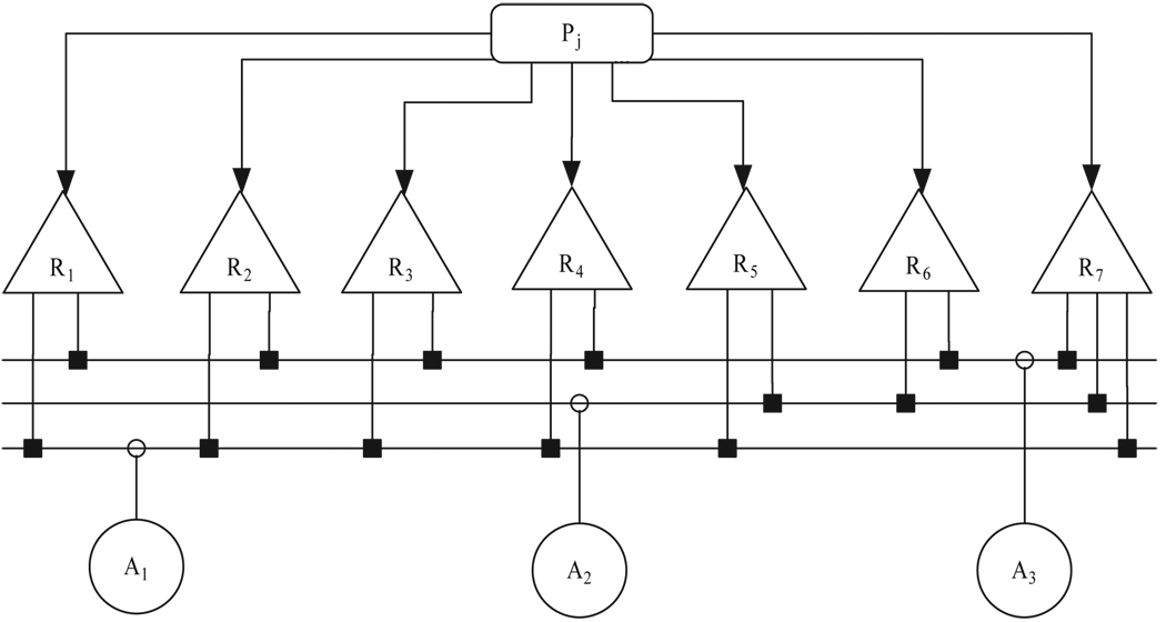
The first step is to identify the risks affecting participant Pj. A risk set R = {R1, …, R7} is identified for a particular participant. Table I contains the description of the risks including the estimation of the occurrence probabilities and their impacts on parental functioning. These values are obtained based on the judgment of clinical staff and the results of a questionnaire completed by one of the parents. This process could be reassessed during each revision period. For risks R1 and R3 the probability of occurrence increases with time; the impact is constant for all the risks and for all revision periods.
TABLE I.
IDENTIFIED RISKS, CASE STUDY. THE VARIABLE t DENOTES TIME.
| Risk | Description | Probability (pi) | Impact (Ii) |
|---|---|---|---|
| R1 | Availability of drugs | 0.5+0.001t | 8 |
| R2 | Family history of problem behavior | 0.01 | 3 |
| R3 | Friends who engage in problem behavior | 0.2+0.001t | 2.7 |
| R4 | Extreme economic deprivation | 0.4 | 3 |
| R5 | Poor family management practice | 0.9 | 4.7 |
| R6 | Lack of commitment to school | 0.2 | 4.3 |
| R7 | Early and persistent antisocial behavior | 0.17 | 2.8 |
Following risk identification, the next task is to define a plan for the mitigation actions that will reduce the impact of the risks. The risk-based structure (RBS) that relates risks and actions is illustrated in Fig. 3. Table II shows the action set A = {A1, A2, A3} to undertake for the mitigation. The intervention potency of action A1 (frequency of home visits) is assumed to be scaled and is defined according to uI(weekly) = 3, uI(biweekly) = 2 and uI(monthly) = 1. Actions A2 (mentoring with contingent reinforcement) and A3 (after-school recreation) are considered to compensate the depletion in parental function as a consequence of the possible risks that could occur. These actions are denoted by the variables uF1 and uF2, respectively. Mentoring is assumed to be scaled according to uF1(weekly) = 3, uF1(biweekly) = 2 and uF1(monthly) = 1. After-school recreation uF2 is expressed as a boolean variable taking the values 1 or 0 for the case of requiring the activity or not, respectively.
Fig. 3.
Risk-based structure (RBS) for the Case Study
TABLE II.
MITIGATION ACTION DESCRIPTION, CASE STUDY.
| Ac | Description | Impact Reduction | Values |
|---|---|---|---|
| A1 | Counselor Home Visits | f1(uI) = 3.9uI | uI ∈ {0, 1, 2, 3} |
| A2 | Mentoring with Contingent Reinforcement | f2(uF1) = 2.4uF1 | uF1 ∈ {0, 1, 2, 3} |
| A3 | After-school recreation | f3(uF2) = 2uF2 | uF1 ∈ {0, 1} |
The system model is based on Equation (5), as described in Section II. Parental function y(t) is treated as a continuous measurement and normalized in the range of 0 to 100%, as described in [11]. The gain and delay values considered are KI = 1.665 and θ = 0, respectively. These values would normally be determined from an efficacy trial or similar study prior to the intervention. The process under analysis is a first-order linear system without dead time and therefore B(q−1) = B0(t). Note that B0(t) is a 3 × 1 matrix and D(t) is a 1 × 1 vector. Next, B0(t) and D(t) are defined as:
| (12) |
| (13) |
The objective function follows (10) with β1 = β2 = 1 and β3 = 0; the cost of mitigation actions is not considered. The constraints that are enforced are the following:
| (14) |
| (15) |
All decision variables in the problem are discrete-valued, but the control error is continuous, resulting in a hybrid MPC controller as noted previously.
A. Test cases
This section describes five simulated scenarios (four nominal test cases and one Monte Carlo) that were done to demonstrate how a risk-based MPC algorithm can be used to control a time-varying adaptive intervention. In all the cases the family receiving the intervention begins with a parental function score at 0. The objective is to reach a parental function of at least 50 percent (yGoal) prior to the third year of the intervention.
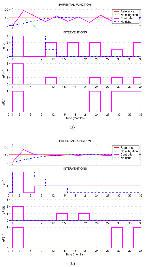
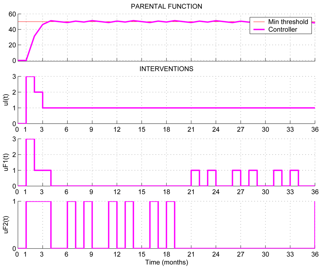
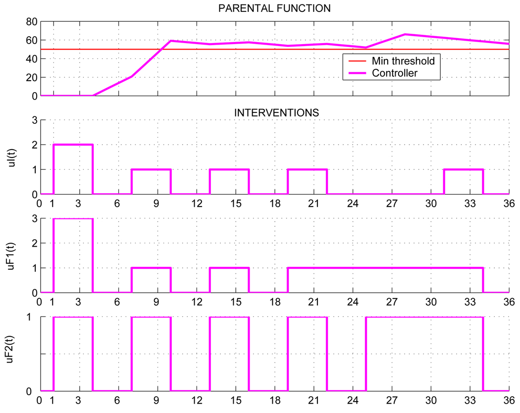
The first test case, represented in Figure 4(a), simulates an adaptive intervention as described in the previous section. The top panel of this figure displays the outcome as a function of time in months. The magenta bold line represents the parental function through the course of the intervention by considering risks. The blue dashed line shows the evolution of the system in the case of no risks, in other words, when the occurrence probabilities of the risks are set to 0. The solid red line is the reference to reach (yGoal). The lower three panels in Figure 4(a) represent the three mitigating actions. The magenta bold line represents the mitigating actions taken in response to risk, and the blue dashed line represents the actions taken by the adaptive intervention when risks are not considered. In both cases, the control system recommends higher dosages during the start of the intervention, which becomes less necessary as parental function improves and reaches towards the goal. The salutary effect of the additional mitigating actions A2 and A3 in the risk-based approach is demonstrated by lower dosages of family counseling needed to achieve a desired parental function goal. However, the adaptive intervention displays oscillatory behavior in parental function and the mitigating actions. This is remedied in Test Case 2, represented in Figure 4(b), by increasing the objective function horizon to N = 5, and increasing the move suppression (λ = 50). The parental function in this tuning of the adaptive intervention settles at the goal much earlier than in Test Case 1, with reduced oscillations in y(t) and greater uniformity in dosage assignments.
Fig. 4.
(a) Results obtained for the MPC controller with base tuning parameters (Test Case 1 N = 1, δ = 1, λ = 10; upper diagram). (b) Test Case 2 results obtained for the MPC controller with improved tuning parameters (N = 5, δ = 1, λ = 50).
Test Case 3 (Figure 5) shows the results that would be obtained if monthly clinical revisions were used in lieu of quarterly ones. The results show that as a result of more frequent revisions, the parental function response experiences less overshoot and reaches the goal in a shorter amount of time. However, the increased number of revisions/faster sampling time demands more effort and resources from the clinical staff in making assessments of parental function and implementing dosage changes. In practice, the benefits of a smoother, more effective intervention would have to be weighted against the extra costs associated with more frequent measurement and faster control action.
Fig. 5.
Test Case 3. Adaptive intervention response in the case of monthly clinical revisions (N = 5, δ = 1, λ = 10)
For Test Case 4, shown in Figure 6, a scenario involving quarterly clinical revisions and time delay of θ = 3 months (one revision period) is evaluated. The control parameters settings are N = 5, λ = 50, δ = 0.5. As in any feedback system, the presence of delay introduces an inevitable lag and degradation in the parental function response; nonetheless, the controller is able to assign dosages of mitigating actions leading to satisfactory outcomes. Because of the discrete-valued nature of the intervention and mitigating actions, perfect setpoint tracking is not accomplished in this case; however, the parental function response has exceeded the goal after only 11 months.
Fig. 6.
Test Case 4. Adaptive intervention response in the case of quarterly clinical revisions and three months (one revision period) delay in participant response (N = 5, λ = 50, δ = 0.5).
B. Monte Carlo Simulation
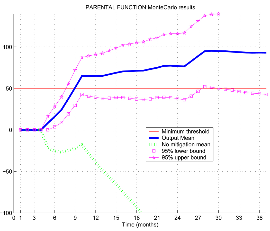
The next experiment shows the results that are obtained when a Monte Carlo simulation is applied. The scenarios have been generated by varying the occurrences of the risks in participants and applying the interventions obtained in the case of quarterly clinical revisions and three month delay (Fig. 6). 200 scenarios are considered following the formula in [30] where a lower bound of the sample complexity is provided in order to be approximately correct to accuracy ε and confidence δ. This bound is polynomial with the dimension of the problem. Figure 7 illustrates the results when Monte Carlo simulation is applied; the parental functioning mean for the different scenarios is the solid blue line. Note that at each monthly time step an identification of the mean and deviation according to a normal distribution has been obtained. The magenta lines with stars and squares represent the upper and lower bound respectively of the 95% interval [μi −1.96σi, μi + 1.96σi] of the output in the scenarios, with μi and σi the mean and deviation in the period i. The dotted green line represents the means of the normal distributions that are obtained for each month in the case of no mitigation.
Fig. 7.
Monte Carlo simulation on the parental function. The solid blue line is the mean of the parental function in each month. The magenta lines with stars and squares represent the upper and lower bound, respectively, of the 95% values in the simulation, for the different scenarios. The dotted green line is the case of no mitigation.
VI. SUMMARY AND CONCLUSIONS
Adaptive interventions individualize therapy by the use of decision rules for how the therapy level and type should vary according to measures of adherence, treatment burden, and response collected during past treatment. This paper describes a control-based methodology for decision-making in adaptive interventions meaningful to addressing prevention and treatment problems in behavioral health. The objective of the control system is to assign dosages of intervention components to achieve a desired participant state, taking into account explicitly modeled risks that can be identified prior to the intervention procedure. By systematically accounting for risks and adapting treatment components over time, an MPC approach as described in this paper has the potential to increase intervention potency and adherence while reducing waste, resulting in more effective interventions than conventional fixed treatment.
Risk modeling involves risk identification, assigning probabilities, and devising a strategic plan to mitigate risks; therefore, getting information from clinical staff and other trained personnel to generate these models is crucial to the success of this approach. Likewise, system identification methods that enable understanding the transient and delayed relationship between intervention dosages and outcomes is a necessary component to this work. In this paper, a hypothetical intervention was developed using information obtained from two real-life programs (Fast Track and Communities that Care) which are associated with the prevention of substance use and conduct disorder in youth and at-risk children.
The presented approach provides recommendations on the actions to undertake in order to mitigate risks that could appear during each review period. Various experiments have been performed corresponding to different scenarios; these include changes in controller tuning, revision periods, and delays in the dynamic response of the interventions. This procedure can be considered as a helpful tool to assist clinicians in evaluating different dosage assignments before providing a definitive intervention to a participant.
VII. ACKNOWLEDGEMENTS
Support for this work has been provided by the Office of Behavioral and Social Sciences Research (OBSSR) of the National Institutes of Health and the National Institute on Drug Abuse (NIDA) through grants R21 DA024266, K25 DA021173 and P50 DA010075. The University of Seville authors would like to thank the Spanish MCYT for funding this work under the grant DPI2008-05818 and P07-TEP-02720.
Contributor Information
Ascensión Zafra-Cabeza, Email: asun@esi.us.es, Escuela Superior de Ingenieros, Department of Automatic Control and Systems Engineering, University of Seville, Camino de los Descubrimientos s/n, 41092 Seville, Spain.
Daniel E. Rivera, Email: daniel.rivera@asu.edu, Control Systems Engineering Laboratory, School for Engineering of Matter, Transport and Energy, Arizona State University, Tempe, Arizona 85287-6106.
Linda M. Collins, Email: lmcollins@psu.edu, Methodology Center and Department of Human Development and Family Studies, Penn State University, 204 E. Calder Way, Suite 400 State College, PA 16801.
Miguel A. Ridao, Email: ridao@esi.us.es, Escuela Superior de Ingenieros, Department of Automatic Control and Systems Engineering, University of Seville, Camino de los Descubrimientos s/n, 41092 Seville, Spain.
Eduardo F. Camacho, Email: eduardo@esi.us.es, Escuela Superior de Ingenieros, Department of Automatic Control and Systems Engineering, University of Seville, Camino de los Descubrimientos s/n, 41092 Seville, Spain.
REFERENCES
- 1.Murphy SA, Collins LM, Rush AJ. Customizing treatment to the patient: adaptive treatment strategies. Drug and Alcohol Dependence. 2007;vol. 88 Supplement 2:S1–S3. doi: 10.1016/j.drugalcdep.2007.02.001. [DOI] [PMC free article] [PubMed] [Google Scholar]
- 2.Collins LM, Murphy SA, Bierman KL. A conceptual framework for adaptive preventive interventions. Prevention Science. 2004;vol. 5(no. 3):185–196. doi: 10.1023/b:prev.0000037641.26017.00. [DOI] [PMC free article] [PubMed] [Google Scholar]
- 3.Glasgow M, Engel B, D‘Lugoff B. A controller study of a standarized behavioral stepped treatment for hypertension. Psychosomatic Medicine. 1989;vol. 51:10–26. doi: 10.1097/00006842-198901000-00002. [DOI] [PubMed] [Google Scholar]
- 4.Rush A, Fava M, Wisniewski S, Lavori P, Trivedi M, Sackeim H, Thase M, Nierenberg A, Quitkin F, Kashner T, Kupfer D, Rosenbaum J, Alpert J, Stewart J, McGrath P, Biggs M, shores Wilson K, Lebowitz B, Ritz L, Niederhe G. Sequenced treatment alternatives to relieve depression (STAR*D): Rationale and design. Controlled Clinical Trials. 2004;vol. 25(no. 1):119–142. doi: 10.1016/s0197-2456(03)00112-0. [DOI] [PubMed] [Google Scholar]
- 5.Sobell M, Sobell L. Changing Addictive Behavior: Bridging Clinical and Public Health Strategies. New York: Guilford Press; 1999. Stepped care for alcohol problems: an efficient method for planning and delivering critical services; pp. 331–343. [Google Scholar]
- 6.Velicer W, Prochaska J. An expert system intervention for smoking cesation. Patient Education and Counseling. 1999;vol. 36:119–129. doi: 10.1016/s0738-3991(98)00129-3. [DOI] [PubMed] [Google Scholar]
- 7.Brooner R, Kidorf M. Using behavioral reinforcement to improve methadone treatment participation. Science and Practice Perspectives. 2002;vol. 1:38–48. doi: 10.1151/spp021138. [DOI] [PMC free article] [PubMed] [Google Scholar]
- 8.Murphy S, McKay J. Adaptive treatment strategies: An emerging approach for improving treatment effectiveness. Clinical Science. 2004 newsletter of the American Psychological Association Division 12, section III: The society for the science of clinical psychology. [Google Scholar]
- 9.Schneider L, Tariot P, Lyketsos C, Dagerman K, Davis K, Davis S, Hsiao J, Jeste D, Katz I, Olin J, Pollock B, Rabins P, Small G, Lebowitz B, Lieberman J. National Institute of Mental Health clinical antipsychotic trials in intervention effectiveness (CATIE) American Journal of Geriatric Psychiatry. 2001;vol. 9:346–360. [PubMed] [Google Scholar]
- 10.Rosenberg E, Altfield M, Poon S, Wilkes M, Eldridge R, Robbins G, D‘Aquila R, Goulder P, Walker B. Inmune control of HIV-1 after early treatment of acute infection. Nature. 2000;vol. 407:523–526. doi: 10.1038/35035103. [DOI] [PubMed] [Google Scholar]
- 11.Rivera DE, Pew MD, Collins LM. Engineering control approaches for the design and analysis of adaptive, time-varying interventions. Drug and Alcohol Dependence. 2007;vol. 88 Supplement 2:S31–S40. doi: 10.1016/j.drugalcdep.2006.10.020. [DOI] [PMC free article] [PubMed] [Google Scholar]
- 12.Litan RE, Krimgold F, Clark K, Khadilkar J. Physical Damage and Human Loss: The Economic Impact of Earthquake Mitigation Measures. Insurance Information Institute; 1992. [Google Scholar]
- 13.Doherty NA. Integrated Risk Management: Techniques and Strategies for Reducing Risk. McGraw-Hill; 2000. [Google Scholar]
- 14.Zafra-Cabeza A, Ridao MA, Camacho EF. An algorithm for optimal scheduling and risk assessment of projects. Control Engineering Practice. 2004;vol. 12(no. 10):1329–1338. [Google Scholar]
- 15.Chapman C, Ward S. Project Risk Management. Processes, Techniques and Insights. 2nd Edition. John Willey and Sons; 2003. [Google Scholar]
- 16.Clarke D. Application of generalized predictive control to industrial processes. IEEE Control Systems Magazine. 1988;vol. 122:49–55. [Google Scholar]
- 17.Herbert RD, Bell RD. Predictive constrained policy generation for macroeconomic systems. Modelling and Control of Economic Systems, SME2001, Preprints. International Federation for Automatic Control. 2001:81–86. [Google Scholar]
- 18.Ginhoux R, Gangloff JA, de Mathelin MF, Soler L, Leroy J, Marescaux J. Surgery Simulation and Soft Tissue Modeling. Lecture Notes in Computer Science. vol. 2673. Heidelberg: Springer Berlin; 2003. Model predictive control for cancellation of repetitive organ motions in robotized laparoscopic surgery; pp. 353–365. [Google Scholar]
- 19.Conduct Problems Prevention Research Group. A developmental and clinical model for the prevention of conduct disorders: The Fast Track program. Development and Psychopathology. 1992;vol. 4:509–528. [Google Scholar]
- 20.Conduct Problems Prevention Research Group. Initial impact of the Fast Track prevention trial for conduct problems: I. The high -risk sample. Journal of Consulting and Clinical Psychology. 1999;vol. 67:631–647. [PMC free article] [PubMed] [Google Scholar]
- 21.Conduct Problems Prevention Research Group. Initial impact of the Fast Track prevention trial for conduct problems: Ii. Classroom effects. Journal of Consulting and Clinical Psychology. 1999;vol. 67:648–657. [PMC free article] [PubMed] [Google Scholar]
- 22.Hawkins JD, Catalano RF, Miller JY. Risk and protective factors for alcohol and other drug problems in adolescence and early adulthood: Implications for substance abuse prevention. Psychological Bulletin. 1992;vol. 112:64–105. doi: 10.1037/0033-2909.112.1.64. [DOI] [PubMed] [Google Scholar]
- 23.Hawkins JD. Preventing crime and violence through communities that care. European Journal on Criminal Policy and Research. 1999;vol. 7:443–458. [Google Scholar]
- 24.Schwartz JD, Wang W, Rivera DE. Simulation-based optimization of model predictive control policies for inventory management in supply chains. Automatica. 2006;vol. 42(no. 8):1311–1320. [Google Scholar]
- 25.Wang W, Rivera DE. Model Predictive Control for tactical decision-making in semiconductor manufacturing supply chain management. IEEE Transactions on Control Systems Technology. 2008;vol. 16(no. 5):841–855. [Google Scholar]
- 26.McKay JR, Lynch KG, Shepard DS, Morgenstern J, Forman RF, Pettinati HM. Do patient characteristics and initial progress in treatment moderate the effectiveness of telephone-based continuing care for substance use disorders? Addiction. 2005;vol. 100(no. 2):216–226. doi: 10.1111/j.1360-0443.2005.00972.x. [DOI] [PubMed] [Google Scholar]
- 27.Zafra-Cabeza A, Ridao MA, Camacho EF, Kempf KG, Rivera DE. Managing risk in semiconductor manufacturing: a stochastic predictive control approach. Control Engineering Practice. 2007;vol. 15:969–984. [Google Scholar]
- 28.Camacho EF, Bordons C. Model Predictive Control. 2nd Edition. London: Springer-Verlag; 2004. [Google Scholar]
- 29.Bemporad A, Morari M. Control of systems integrating logic, dynamics, and constraints. Automatica. 1999;vol. 35(no. 3):407–427. [Google Scholar]
- 30.Vidyasagar M. A theory of learning and generalization. London: Springer-Verlag; 1997. [Google Scholar]


