Large-Scale Clustering of cDNA-Fingerprinting Data

Abstract

Clustering is one of the main mathematical challenges in large-scale gene expression analysis. We describe a clustering procedure based on a sequential k-means algorithm with additional refinements that is able to handle high-throughput data in the order of hundreds of thousands of data items measured on hundreds of variables. The practical motivation for our algorithm is oligonucleotide fingerprinting—a method for simultaneous determination of expression level for every active gene of a specific tissue—although the algorithm can be applied as well to other large-scale projects like EST clustering and qualitative clustering of DNA-chip data. As a pairwise similarity measure between two p-dimensional data points, x and y, we introduce mutual information that can be interpreted as the amount of information about x in y, and vice versa. We show that for our purposes this measure is superior to commonly used metric distances, for example, Euclidean distance. We also introduce a modified version of mutual information as a novel method for validating clustering results when the true clustering is known. The performance of our algorithm with respect to experimental noise is shown by extensive simulation studies. The algorithm is tested on a subset of 2029 cDNA clones coming from 15 different genes from a cDNA library derived from human dendritic cells. Furthermore, the clustering of these 2029 cDNA clones is demonstrated when the entire set of 76,032 cDNA clones is processed.

The method of hybridization of short synthetic oligonucleotide probes to cloned cDNA sequences under high stringency conditions to extract genetic information has been demonstrated by a number of research groups in recent years (Lehrach et al. 1990; Lennon and Lehrach 1991; Meier-Ewert et al. 1993; Drmanac et al. 1996; Milosavljevic et al. 1996). Oligonucleotide fingerprinting is an efficient and fast approach to extract parallel gene expression information about all genes that are represented in a cDNA library from a specific tissue under analysis. To ensure that the cDNA library is representative for gene expression, which means that the number of genes active in the tissue and their corresponding expression rates are reflected, its size has to be in the order of 100,000–200,000 cloned sequences, because we expect the number of active genes in most tissues at most stages of development to be 10,000–30,000 with abundance varying from 1 (singleton) to 1000. The cloned sequences (clones) are amplified by PCR, immobilized on nylon filter membranes (25,000 different clones per filter membrane), and hybridized in parallel to a radioactively labeled oligomer probe of known sequence. After a scanning procedure, image analysis software developed in-house (unpublished) evaluates the hybridization experiment by assigning each clone a numerical value that is proportional to the amount of bound radioactively labeled probe. By repeating this experiment with different probes (100–300), each clone is described by a characteristic vector of numerical values—subsequently called a fingerprint. Detailed protocols of the procedure including possible quality checks have been published (Maier et al. 1994; Schmitt et al. 1999; Clark et al. 1999).

Because of the use of hundreds of different probes, we can assume that the fingerprint is characteristic for the individual clone sequence, although there is a certain loss in information by representing sequences by fingerprints. An advantage of the fingerprinting procedure, however, is that it takes into account the whole clone sequence and is therefore more sensitive in gene discrimination than, for example, EST approaches in which only end sequences from one or both ends are used for pairwise clone comparison (Adams et al. 1991, 1993).

The task of the clustering procedure is to classify the clone fingerprints according to a well-defined pairwise similarity measure to group similar fingerprints together and to separate dissimilar ones. The calculated classification reflects the number of different genes expressed in the tissue (number of clusters) and their relative abundance (size of clusters). Clustering results help normalize cDNA libraries and thus significantly reduce sequencing effort in gene identification. When processing tissues from different developmental stages, clustering can detect differences in gene expression and thus identify development-specific genes. A pilot study has been published recently (Meier-Ewert et al. 1998). A practical clustering procedure has to consider several experimental requirements. The main demand is the ability to handle data sets in the order of hundreds of thousands of high-dimensional data points in an acceptable amount of time. A further requirement on the algorithm is the ability to work with partial information in the form of missing values. In real experiments this is necessary because common data sets contain a certain amount of missing values (up to 25%), because, for example, the set of probes may vary when comparing different cDNA libraries and the reproducibility of hybridization signals can be poor (see Methods). This problem is mainly addressed to the pairwise similarity measure in use that must be able to assign comparable similarity values even when part of the data is missing. Finally, the algorithm should be robust enough to cope with experimental noise because high-throughput data is usually generated within a production pipeline that involves many different steps and is therefore somewhat error prone.

We focus here on a partitioning algorithm with heuristic modifications that finds the number of cluster centroids from the data itself and a “good” partition according to these centroids. Additionally, we present a suitable pairwise similarity measure based on mutual information that fits the above-mentioned requirements. Our algorithm has been extensively tested on simulated and experimental data sets. We describe simulation studies based on real sequence data from GenBank/EMBL database sequences to test the performance on important error parameters (false-positive rate, false-negative rate, length variation of cDNA clones). To quantify the quality of the calculated partitions, we introduce a novel measure for cluster validity based on a modified version of mutual information: the relative mutual information coefficient (RMIC). Additionally, we run the algorithm on a data set of 2029 cDNA clones from 15 genes extracted from a human cDNA data set containing a total of 76,032 cDNA clones. Furthermore, the clustering of these 15 gene clusters is shown when the entire set of 76,032 cDNA clones is processed. We are able to produce highly pure gene clusters out of such large data sets even when clusters are small (<15 copies). The results show that our method is a robust, fast, and accurate way to process large data sets and that it can be applied to major problems of gene expression analysis like gene identification and comparative gene expression profiling.

RESULTS

All mathematical definitions and technical terms are introduced in Methods. There, we describe a clustering algorithm and a pairwise similarity measure based on mutual information that is superior to commonly used metric distances as is shown below. To validate clustering results when the true clustering is known, we introduce a novel measure for clustering validity: the RMIC.

Advantages of Mutual Information Similarity Measurement

Using mutual information as a pairwise similarity measure for fingerprinting data outperforms commonly used metric distances like Euclidean distance (see Methods). One major advantage is the fact that mutual information takes into account the total number of matched similarities, whereas distance metrics do not. Consider for example the following fingerprints: x₁ = (1,0,0,0,0,0,0,0,0,0); x₂ = (1,1,0,0,0,0,0,0,0,0); x₃ = (1,1,1,1,0,0,0,0,0,0); x₄ = (1,1,1,1,1,0,0,0,0,0).

Here, the individual signals are binarized for simplification; clearly, Euclidean distance of x₁ and x₂ as well as of x₃ and x₄ is equal to 1, which means that a rather nonspecific similarity (which is a dissimilarity in the case of a metric) based on one match equals a far more specific similarity based on four matches. In contrast, mutual information takes into account the number of matches so that the similarity of x₁ and x₂ is lower than the similarity of x₃ and x₄. This is true because mutual information quantifies the global correlation between signal vectors and not only the dissimilarities. A further disadvantage of Euclidean distance is the fact that very uninformative fingerprints (those that match only to a few probes) get a high pairwise similarity (low pairwise distance) just because of the absence of high signal values even if they are from totally different DNA sequences. This seriously affects clustering by grouping many uninformative fingerprints around the zero vector. Mutual information of pairs of uninformative and different fingerprints, on the other hand, is very low as should be the case. Furthermore, we do not have an easy and defined way to handle missing data when using a metric distance. Some methods have been suggested (Jain and Dubes 1988), but as they are all based on estimation of the missing data by the existing data, this leads to unpredictable influences. By taking into consideration only those signals that are present in both vectors, mutual information weights the data implicitly. In other words, missing values are treated as they should be: They are ignored.

Assessing Clustering Quality

RMIC is easy to interpret and has the same range (the interval [−1,1]) for all underlying true clusterings. This makes calculations with different true clusterings more transparent and comparable. Our simulation results (Fig. 1) indicate that the tendency of RMIC compared with the relative Minkowsky metric using a fixed true clustering is fairly similar, that is, RMIC is high where relative Minkowsky metric is low, and vice versa. On the other hand, a concrete value of relative Minkowsky metric is not easy to interpret because the range of the quality measure is extremely sensitive to the complexity of the underlying true clustering. Assume a data structure of N data points and let the true clustering be the trivial clustering in which each data point is a singleton and let the calculated clustering be the trivial clustering in which all N data points are falsely clustered in one big cluster, then the relative Minkowsky metric equals

. If, on the other hand, the true clustering is the trivial clustering in which all data points belong to one cluster and if the calculated clustering is the trivial clustering in which each data point is falsely clustered as a singleton, we get

for relative Minkowsky metric. However it is not quite clear why the latter situation should be weighted so well compared with the former. RMIC, on the other hand, values both situations equally; we have 0 in both cases.

Figure 1.

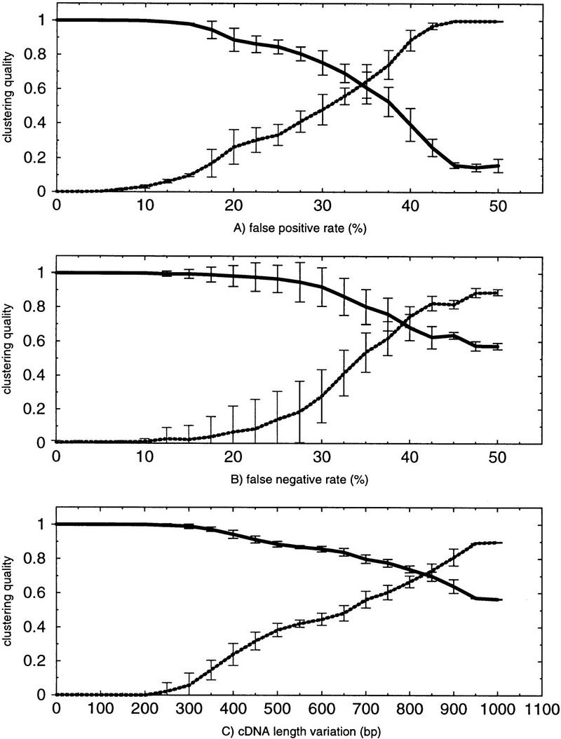
Simulation studies. Clustering is tested on three error parameters: (A) false-positive rate, (B) false-negative rate, and (C) cDNA length variation. False-positive rate and false-negative rate are measured in percents, and length variation is measured in base pairs. Clustering quality is calculated according to two different quality measures: (Broken lines) The relative Minkowsky metric, which is low if clustering quality is good and high if clustering quality is bad; (solid lines) the RMIC, which is high if clustering quality is good and low if clustering quality is bad. For each parameter size, 20 independent clusterings are performed to derive the mean (μ) and the s.d. (σ). The bars indicate the interval [μ − σ, μ + σ].

Simulation Setup

To simulate the robustness of our clustering procedure against experimental noise, we extract 698 different genes from GenBank/EMBL databases. Only sequences longer than 500 bp are considered; sequences longer than 2000 bp are cut at that level so that the actual length of the sequences is between 500 and 2000 bp. This reflects our experimental observation in which we find the average length of clone inserts to be ∼1400 bp with moderate variations. From each gene we produced a specific number of copies ranging in size from 491 down to 1 so that we ended up with a total of 6309 sequences. Table 1 shows the distribution of gene copy numbers.

Table 1.

Distribution of Gene Copies for Simulation

	Cluster size
1	2–5	6–10	11–100	>100	total
No. of cluster	500	144	21	16	17	698
No. of clones	500	388	156	381	4884	6309
Percent of sample	7.93	6.15	2.47	6.03	77.41	100

A total of 665 out of 698 genes are assigned a copy rate <11 (including 500 singletons) corresponding to a total number of 1044 clones; 17 genes get a copy rate >100 by a random number between 100 and 500. The biggest of our simulated cluster has a copy rate of 491 clones. 

A total of 147 octamer probes—a subset of those probes used in our experiments—are chosen for determining theoretical fingerprints. Hybridization results are computed as 1 or 0 for a match of the probe (or its reverse complementary sequence) with the gene sequence or not, respectively. The matching rates of the probes differ between 5% and 35% (20% on average).

We test the algorithm on three main error parameters, namely, false positive rate, r_p; false negative rate, r_n; and cDNA length variation, Δ: If A is the event that we observe a positive hybridization experimentally and B is the event that there is a theoretical match by sequence and A and B are the respective complementary events, then we straightforwardly define r_p = prob(A|B) and r_n = prob(A|B) as false-positive rate and false-negative rate, respectively. Error is introduced independently for each probe, which fits our experimental situation. Length variation, Δ, of the cDNA clones is due to the fact that reverse transcriptase stops at different end points when processing cDNA from mRNA during transcription; therefore, cDNA copies of the same gene will in principle have different lengths. If, due to high length variation, the sequences do not share enough probe matches, clustering of the respective copies of the same gene might fail. Length variation is introduced in a uniform way: For each gene, g_i, with length, l_i, and for each length variation parameter, Δ, we choose the end points of the copies of that gene uniformly within the interval (max{0,l_i − Δ},l_i).

Figure 1 shows the performance of the algorithm on these parameters. For each parameter value, 20 independent simulation runs were calculated to derive the mean (μ) and the standard deviation (σ). The bars indicate the interval [μ − σ,μ + σ]. We measure cluster quality in two alternative ways: The broken lines show the Minkowsky metric and the solid line our RMIC. We observe that the procedure is less sensitive to false-negative than to false-positive error. This is due to the high a priori probability of a negative sequence match. High quality can be observed if the false-positive rate is <30% and the false negative rate is <35%. False-negative rates up to 20% and false-positive rates up to 15% have extremely low influence; cluster quality is nearly perfect (0.98 for RMIC in both cases and 0.07 and 0.1 for Minkowsky metric). Quality is significantly reduced if false-positive error is between 30% and 45% and false negative error is within 35%–50%, although the algorithm is clearly robust to such high noise: For example, a false positive rate of 35% leads to a quality index of 0.61, which indicates that the clustered partition contains a large amount of information about the true clustering and which is still sufficiently high to observe good results in practice. This is remarkable because a false-positive rate of 35% according to the above definition means that a proportion of 28% (35% of 80%) of all signals on average is falsely set to 1 (in contrast to 20% of all signals on average that remain correctly set to 1), so that more positive signals in the data set are false than are true. This is due to the dissimilar a priori probabilities of positive and negative theoretical sequence match. Length variation is a serious problem; clustering quality remains stable if variation is below 500 bp (0.89 for RMIC and 0.38 for Minkowsky metric) but decreases significantly if the variation is larger than 700 bp. Experimental improvements are ongoing to overcome this kind of error (see Discussion).

Clustering Human cDNA Clone Fingerprints

The cDNA library under analysis is derived from human peripheral blood dendritic cells. Dendritic cells have a key role in the immune system through their ability to present antigen. From the clustering point of view, the complexity of the library is interesting: As these cells are specialized to certain biological processes, we estimate the number of different genes to be ∼15,000, although there is no exact data available.

To test the algorithm on experimental data, 15 different cDNA clones are partially sequenced, identified, and, afterwards, hybridized to the entire cDNA library, and a total set of 2029 cDNA clones are extracted that give strong positive signals with one of the genes. The distribution of gene copies is shown in Table 2. Most of the control genes are house-keeping genes that are present with a moderate to high copy rate. Elongation factor α, for example, is the most frequent gene with 669 copies, which is a proportion of 0.876% of the entire library and 32.82% of the selected subset. Gene copy sizes for three of the control genes are <15.

Table 2.

Distribution of Control Gene Clusters

NR.	Gene ID	Copies	Subset (%)	Library (%)
1	Ef1_α	669	32.82	0.876
2	Cytochrom_cox_I	274	13.55	0.362
3	clone_190B1	254	12.52	0.334
4	tubulin_β	207	10.20	0.272
5	40SRibo_protS6	183	9.02	0.241
6	40SRibo_protS4	100	4.93	0.132
7	60SRibo_protL4	85	4.24	0.113
8	GAPDH	82	4.04	0.108
9	Ef1_β	67	3.30	0.088
10	human_calmodulin	32	1.58	0.042
11	heat_shock_cogKD71	28	1.38	0.037
12	heat_shock_cogKD90	26	1.28	0.034
13	human_TNF_receptor	12	0.59	0.016
14	clone_244D14	8	0.44	0.012
15	clone_241F17	2	0.10	0.003
Total		2029	100	2.67

The entire human cNDA clone set contains 76,032 clones. The subset of the control gene cDNA clones contains 2,029 clones. Most of the control genes are house-keeping genes that have a moderate to high copy rate although three of the genes have a copy rate <15. The copies of the subset sum to a proportion of 2.67% of the entire library. 

The library is hybridized with 200 octamer probes. These probes are selected on the basis of ∼15,000 human sequences extracted from GenBank/EMBL databases. Probes are chosen according to the following iterative procedure (A.O. Schmitt, pers. comm.): Given a set S of probes to select from, (1) start with the probe in S that best partitions the database sequences into two groups. (2) Given a selected set of k probes that best partitions the test set into 2^k partitions, add to the list the probe that—together with the previously selected ones—best partitions the test set into 2^k+1 partitions using entropy of the partitions as quality criterion. This leads to a set of probes that is highly informative for discriminating known genes; we assume however that the database (and thus the computed probe set) is representative for all human genes.

Clustering of the 2029 clones takes <2 min on a Digital-Alpha 500-MHz computer. Twenty-three clusters are found; 45 clones remain as singletons. The quality values are 0.80 for RMIC and 0.37 for Minkowsky metric. Table 3 shows the splitting of the gene clusters. To evaluate the splitting of individual gene clusters numerically, we calculate a diversity index using entropy. Given that gene, g_i, is present in the library with N_i copies and given that these copies are split in K different clusters with frequencies n₁, … ,n_k (n₁+ … +n_k = N_i), then the diversity of the clustering with respect to this gene can be calculated as

The diversity is maximal [δ(g_i) = 1] if all copies belong to different cluster, it is minimal [δ(g_i) = 0] if all copies belong to the same cluster.

Table 3.

Cluster Splitting of Gene Clusters Within 2.029 cDNA Clones

Gene ID	Copies	Core clusters	Total	Percent of copies	Diversity index
Ef1_α	669	636 (646), 3 (4)	639	95.52	0.049
Cytochrom_cox_I	274	229 (232), 24 (24),  12 (14), 2 (2)	267	97.45	0.121
clone_190B1	254	237 (241), 2 (2)	239	94.09	0.068
tubulin_β	207	203 (205)	203	98.07	0.023
40SRibo_protS6	183	176 (176)	176	96.17	0.045
40SRibo_protS4	100	99 (99)	99	99.00	0.012
60SRibo_protL4	85	84 (86)	84	98.82	0.014
GAPDH	82	77 (77)	77	93.90	0.074
Ef1_β	67	66 (76)	66	98.51	0.018
human_calmodulin	32	22 (26), 4 (4)	26	81.25	0.324
heat_shock_cogKD71	28	22 (23)	22	78.57	0.271
heat_shock_cogKD90	26	20 (20)	20	76.92	0.276
human_TNF_receptor	12	8 (8)	8	66.67	0.442
clone_244D14	8	3 (3)	3	37.50	0.318
clone_241F17	2	2 (2)	2	100.00	0.000
Total	2029		1932	95.22	0.137

The diversity index for most gene clusters is low (< 0.2). E.g., GAPDH (human glyceraldehyde-3-phosphate dehydrogenase) is present with 82 copies in the library. Clustering finds 77 copies in a calculated cluster of size 77 (the numbers in brackets denote the sizes of the calculated clusters). These 77 copies correspond to 93.90% of the copies of that gene. We consider only calculated clusters that are pure because only those clusters contribute to gene identification. 

For each gene we count the number of identified clones, whereby only clones from its core clusters (clusters that are pure with respect to that gene) within the calculated partition are considered because only clones from core clusters have a chance of being detected and identified when extracting a small number of clones for sequencing. The gene tubulin_β, for example, is present in 207 copies, 203 of which are in a cluster of size 205 (which is a pure cluster then with respect to this gene); these 203 clustered copies correspond to a total fraction of 98.07% of all copies of that specific gene; 4 copies are split in other clusters. The diversity for tubulin_β is 0.023, which is very small. Our partition leads to a fraction of 95.22% of clones that fall into pure clusters. Twenty calculated clusters have a purity above 85% (corresponding to 95.02% of all clones), and 11 calculated clusters are totally pure; that is, all clones within these clusters belong to the same gene. Only two calculated clusters have a purity below 70%, they contain a mixture of clones from several genes and do not contribute to gene identification. False assignment to singletons happened in 45 cases (2.2%). This is due rather to false hybridization and to false evaluation of this hybridization than to clustering error because the similarities of these clones to clones from the core clusters are very low. However, all 15 genes could have been identified by sequencing a small number of clones from each calculated cluster. Reduction in sequencing effort would have been 91%.

Table 4 shows a contingency table of the calculated and the true partitions. We observe an overestimation of the total number of genes by a factor of 1.53 (see Discussion) due to stringently set algorithmic parameters. Here, rows correspond to calculated clusters; columns correspond to true clusters.

Table 4.

Contingency Table of Calculated and True Partitions

	1	2	3	4	5	6	7	8	9	10	11	12	13	14	15	Total
1	636	1	1											5		643
2	1		237					1		2						241
3	1	229	1										1			232
4	1			203	1											205
5					176											176
6						99										99
7	1				1		84									86
8								77								77
9	1		7	1		1			66							76
10	4									22						26
11		24														24
12					1						22					23
13												20				20
14	10			1				1			1	2				15
15		12		1					1							14
16													8			8
17										4						4
18	3		1													4
19														3		3
20		2														2
21	1						1									2
22			2													2
23															2	2
24(*)	10	6	5	1	4			3		4	5	4	3			45
Total	669	274	254	207	183	100	85	82	67	32	28	26	12	8	2	2029

Rows correspond to calculated clusters; columns correspond to true clusters. We observe a high proportion of pure calculated clusters. Only two clusters (cluster 14 and cluster 21) have a purity below 70%. Cluster 24 is marked (*). It contains singletons, i.e., clone fingerprints that have not been assigned to any of the clusters. False assignment to singletons happened in 45 cases (2.2%). 

The entire gridded human cDNA library contains 76,032 clones after the normalization procedure (see Methods). Clustering takes ∼55 hr on a Digital-Alpha 500-MHz computer. This run time can rapidly be decreased by clustering buffers of 25,000 clones each on multiple processors in parallel and then reclustering the calculated centroids from the buffers. Using four of the above-mentioned processors in parallel decreases run time to 25 hr.

Table 5 shows the cluster splitting of the 15 control genes. We observe an increase in cluster splitting due to stringently set algorithmic parameters. This is necessary because the distribution of cluster sizes in the entire library differs fundamentally from that of our subset. Most genes are expected to appear at low copy rates (1–20) and only a few of them at copy rates >100. To detect low-copy genes, the algorithmic parameters have to be set quite stringently to guarantee high purity even in small clusters. Clustering finds a total of 7391 clusters and 16,287 singletons. There is a certain overestimation of the number of genes due to cluster splitting and false assignment of clones to singletons. On the other hand, as most of the genes are low-copy genes, the splitting is less serious than it seems when judged by our control genes because of their high copy rates. Most core clusters are smaller (cf. with Table 3) as 5%–15% fewer copies are identified. Diversity increases moderately although one gene (human_TNF_receptor) is split to a high degree. False assignment to singletons happened in 53 cases (2.6%). Again, all 15 genes could have been identified by sequencing a small number of clones from each cluster—even those with small copy rates. It is also remarkable that the two-copy gene clone_241F17 has been found correctly out of a pool of 76,032 cDNA clones.

Table 5.

Cluster Splitting of Gene Clusters Within 76,032 cDNA Clones

Gene ID	Copies	Core clusters	Total	Percent of copies	Diversity index
Ef1_α	669	319 (396), 209 (225), 9 (13),  4 (4), 2 (3), 2 (2), 2 (2)	549	82.06	0.303
Cytochrom_cox_I	274	217 (225), 20 (23), 2 (2)	239	87.23	0.199
clone_190B1	254	218 (264), 5 (5)	223	87.80	0.159
tubulin_β	207	195 (199)	195	94.20	0.067
40SRibo_protS6	183	161 (161), 6 (7)	167	91.26	0.129
40SRibo_protS4	100	83 (83), 5 (6)	88	88.00	0.183
60SRibo_protL4	85	70 (103)	70	82.35	0.162
GAPDH	82	72 (78)	72	91.14	0.148
Ef1_β	67	63 (69)	63	94.03	0.073
human_calmodulin	32	14 (15), 3 (3)	17	53.13	0.637
heat_shock_cogKD71	28	15 (17)	15	53.57	0.565
heat_shock_cogKD90	26	18 (19)	18	69.23	0.386
human_TNF_receptor	12	2 (2), 2(2)	4	33.33	0.907
clone_244D14	8	4 (4)	4	50.00	0.469
clone_241F17	2	2 (2)	2	100.00	0.000
Total	2029		1720	84.77	0.292

The gene 40SRibo_protS6 (human ribosomal protein S6 gene) is split into two clusters. One hundred sixty-one copies are clustered in a cluster of size 161 (numbers in brackets refer to the calculated cluster sizes), and 6 copies are clustered in a cluster of size 7. Together, 167 copies of that gene can be identified, which is a proportion of 91.26% of all copies of that gene. The rest of the copies are split into other clusters; the diversity index is 0.129, which is still low. 

The robustness of our clustering procedure is also demonstrated by visualizing clone fingerprints that are clustered together. Figure 2 shows a calculated cluster of size 69 in which 63 clones correspond to the gene Elongation factor β. We see that a set of ∼15 probes (7.5% of all probes) that are common for nearly all clones is sufficient to cluster those clones correctly from 76,032 other fingerprints. We also observe that there are a lot of additional hybridizations not common to all clones in every clone fingerprint (due to false positive hybridizations or length variation), but as these signals are distributed arbitrarily among the probes, clustering is not affected seriously.

Figure 2.

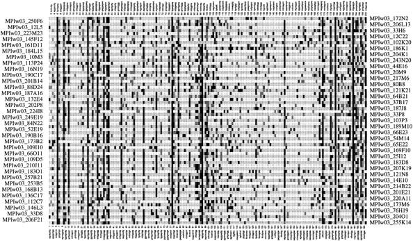
Visualization of calculated cluster. A calculated cluster of size 69 that contains 63 clones from the gene Elongation factor β. Rows (left and right) correspond to clone names (internal abbreviations), and columns (top and bottom) refer to the hybridized probes. Different gray levels are introduced according to the strength of the individual hybridization signal (black = strong signal).

Comparison of Similarity Measures

The subset of 2029 control clones is used to compare the mutual information similarity measure with Euclidean distance and Pearson correlation. Given two vectors and x = (x_l, … ,x_N) and y = (y_l, … ,y_N), Euclidean distance is defined in Methods, and Pearson correlation is given by the formula

in which x_m and y_m are the respective means of the vectors. Using our clustering algorithm with Euclidean distance as similarity measure (which is a dissimilarity in this case), we obtain 30 clusters and 115 singletons, which leads to an overall quality of 0.76 for RMIC and 0.43 for Minkowsky metric. Using the Pearson correlation measure, clustering finds 29 clusters and 78 singletons corresponding to an RMIC of 0.81 and a Minkowsky metric of 0.39. Figure 3 shows the comparison of diversity indices for Pearson correlation, Euclidean distance, and mutual information. It is observable that mutual information gives the best results for most genes compared with the other two measures, whereas Euclidean distance is the weakest of the three measures; although for two genes (Cytochrom_cox_I and Elongation factor β) it is considerably better than the two others. Pearson correlation is nearly as good as mutual information, but regarding the number of singletons and the number of calculated clusters, we think that mutual information is superior especially when taking into consideration the size of common data sets.

Figure 3.

Comparison of similarity measures. Diversity indices describing the cluster splitting of 15 control genes when using Euclidean distance (dotted line), Pearson correlation (solid line), and mutual information (dot-dashed line) as pairwise similarity measures. x-Axis shows the number of the respective gene; y-axis shows the diversity. Diversity is 0 if all copies are clustered in the same cluster; it is 1 if all copies are split into different clusters.

DISCUSSION

Our assumptions are quite general. Hybridization experiments can be viewed as independent of each other if the probes in use are different enough in their sequences. In practice, probes differ in hybridization frequency, reproducibility, and hybridization quality. From theory it is clear that the most informative set of probes would have an average matching frequency of 50%, but in practice the matching frequency of octamer probes is much lower. We estimate (e.g., by evaluating control clones of known sequences) the range of positive hybridizations of the probes to be 5%–25%. Two different approaches could lead to the design of probes with higher matching rates: (1) The use of shorter probes than octamers increases matching frequencies statistically; Milosavljevic et al. (1996) and Drmanac et al. (1996) have shown that it is experimentally possible to hybridize and to evaluate heptamer probes. (2) The pooling of octamer probes is another way to increase matching frequencies. Our probes are pools of 16 different decamer probes with the same 8-mer core sequence (Meier-Ewert et al. 1998). Pooling could be generalized to use probes that differ to a greater degree. However, the choice of pools is difficult and far from routine. It is, on the other hand, desirable in some situations to have low matching frequencies to derive very specific hybridization matches, for example, when working with motif probes that are specific for a small proportion of cDNAs.

It has been shown that the use of mutual information as a pairwise similarity measure for clone fingerprints has several advantages compared with commonly used distance measures. To estimate the joint distribution of a pair of data points by relative frequencies it is necessary to define a finite number of intervals that determine the joint events. The number of intervals should be moderate enough to allow good estimates. We set the number to 5 (corresponding to 25 joint classes), which has been performed best by running several data sets with different class sizes. The number of intervals affects the data in the same sense as the number of bins affects the computation of a histogram: If on the one hand the bin width is too small, most values fall in different bins so that no meaningful compression of data is possible; if on the other hand the bin width is too big, essential differences of data distribution disappear. There is no optimal choice for each data set, it is, for example, dependent on the way of normalization of the data and on the individual biological application so that the best number should be obtained heuristically by running the algorithm several times. For our application five intervals are sufficient, but, for example, for gene expression analysis the number might be enlarged. Theoretically, it is straightforward to derive a quantitative analog of mutual information by extending entropies to differential entropies, but for practical purposes this is less appropriate. On the other hand when investigating time-dependent differences of gene expression ratios, questions are rather of qualitative nature, and mutual information can be used to measure pairwise gene regulation information described by qualitative levels of gene expression like up-regulated, down-regulated, or unchanged (compared with a reference level). An interesting application of mutual information analysis in the context of genetic networks is described by Liang et al. (1998).

Further improvements on pairwise clone fingerprint similarity can be made. One shortcoming of the measure is that all pairwise events are weighted equally regardless of their information content. For example, the event that both clones do not match with a given probe gets the same weight as the event that both clones do although the latter information is far more important than the former one due to the dissimilar a priori probabilities of a match and a nonmatch, respectively. This can be taken into account by using a weighted form of mutual information in which the joint events are weighted, and these weights are directly proportional to the importance of the joint events. The weights depend hereby on the specific set of probes and the clones under analysis.

Experimental observations show that in most cDNA libraries there is a small number of big gene clusters and a high number of singletons and small gene clusters (Meier-Ewert et al. 1998; Poustka et al. 1999). We observe that, in general, big clusters are easy to identify by clustering procedures as centroids can be moved in the right direction because variance in the signals gets smaller, whereas small clusters are harder to identify because of the high variance introduced by experimental error. The identification of small clusters needs the generation of highly pure clusters by stringently set algorithmic parameters. This leads to an overestimation of the total number of genes due to cluster splitting and to the false assignment of clones to singletons that should be clustered and thus to a lower normalization rate of the cDNA library. The estimated proportion of false-positive assignments of clones to singletons is 3%; that is, 3% of the clones that should be clustered remain as singletons. However, by extracting a clone from each cluster it is possible to get a three- to fourfold normalization of the initial library and to identify almost all active genes in the tissue.

There are several alternatively usable clustering procedures. One usually distinguishes between two main classes of clustering procedures; partitioning and hierarchical methods. Partitioning methods try to find the “best” partition given a fixed number of classes, whereas hierarchical methods calculate a full series of partitions starting from N clusters each of which contains one single data point and ending with one cluster that contains all points (or vice versa); in each step of the procedure, two clusters are merged according to a prespecified rule. In general, hierarchical methods suffer from the fact that they do not “repair” false joining of data points from previous steps; indeed, they follow a fixed path for a given rule (Kaufman and Rousseeuw 1990). Furthermore, the display of hierarchical methods—commonly given in form of a dendrogram that resembles a phylogenetic tree—is very hard to interpret when data size is large. Hierarchical methods have recently been applied mainly in the context of gene expression analysis: Eisen et al. (1998) use a hierarchical clustering method based on pairwise average-linkage analysis. Pairwise similarities are calculated according to a measure of correlation that is an extension of the Pearson correlation coefficient. Wen et al. (1998) use the FITCH algorithm (Felsenstein 1993) to produce a phylogenetic tree from a distance matrix derived from pairwise Euclidean distances. Alon et al. (1999) use deterministic annealing to calculate a binary tree and recalculate clusters from this tree—a fast and efficient algorithm that scales N log (N) and does not require the calculation of all pairwise similarities. Many clustering algorithms are based on graph theory approaches, in which nodes of the graph correspond to data points and edges are weighted according to pairwise similarities. Interesting algorithms based on threshold graphs are shown by Hartuv et al. (1999) and Ben-Dor and Yakhini (1998). The latter approach is enriched by heuristics that allow corrections of false joining of two data points. Another interesting approach to clustering are self-organizing maps. Recent studies have been published in the context of gene expression analysis (Tamayo et al. 1999; Törönen et al. 1999).

Common criticism of k-means algorithms centers on the fact that the number of centroids has to be fixed from beginning of the procedure; thus the results are highly dependent on the initialized set of centroids. This version of k-means was recently applied in a study by Tavazoie et al. (1999) in which Euclidean distance as pairwise distance measure is used. Here, we present a sequential k-means approach that has been introduced by MacQueen (1967) and further described by Mirkin (1996) that finds the number of different clusters from data itself and is independent of a prespecified number of centroids. The simulation studies show that the variance of clustering quality for each parameter is fairly small and indicate that the random initialization of different centroids for each simulation run does not change clustering results tremendously. Further application of the algorithm to various cDNA libraries of different organisms including human, mouse, zebrafish, sea urchin, and amphioxus shows that the procedure of determining algorithmic parameters can be set quite generally independently of the cDNA library.

The sequential structure of our algorithm allows the analysis of even larger data sets in a reasonable amount of time by splitting the data in smaller data sets, clustering these sets in parallel using multiple processors, and then reclustering the calculated centroids. This procedure reduces computation time to a high degree because the time-consuming step of finding the centroids in the data can be computed in parallel. This procedure has been applied to 200,000 clones from two human cDNA libraries where run time was <3 days (65 hr) using four processors in parallel with eight buffers of 25,000 clones each. For further attempts we estimate the run time for 400,000 clones to be <5 days (100 hr), for 800,000 clones to be ∼1 week (175 hr), and for 1,600,000 clones to be <2 weeks (325 hr), corresponding to 4, 8, and 16 representative cDNA libraries. Taking into account the rapid development in computer hardware, these run times are upper bounds for the future.

A significant reduction of cluster quality is observable if length variation of cDNA clones is >700 bp. Improvements have to be made to increase robustness on this kind of error. A straightforward way to overcome this problem is the use of more probes. Attempts are ongoing to increase hybridization number per clone by 50–100 more probes. This will also improve separation and identification of partially overlapping genes such as splice variants and highly homologous genes. These are experimental improvements that do not involve changes within the algorithm.

An important aspect in future work will be the establishment of clone fingerprint databases and their statistical evaluation for gene identification. Depending on the reproducibility of hybridization signals and depending on normalization procedures, it will be possible to compare cDNA fingerprints from different tissues of an organism. The number of unknown and unidentified genes will thereby be reduced significantly; verified knowledge on known genes can be used to identify unknown genes.

Although we focus here on cDNA fingerprint data, the algorithm and the pairwise similarity measure are in no way restricted to this kind of data and might be applied to other genetic large-scale projects. Preselection of clones from shotgun libraries of genomic DNA with oligonucleotide fingerprinting has been published recently (Radelof et al. 1998). This can be done by using the clustering algorithm to reduce redundancy from highly overlapping clones. The sequential structure of the algorithm offers the possibility to process very large shotgun libraries, for example, covering an entire chromosome. Another possible application is sequence comparison by theoretically fingerprinting EST sequences using our approach. Attempts in this direction are ongoing (R. Herwig, unpubl.).

METHODS

Source of Biological Material

The cDNA library under analysis is derived from human peripheral blood dendritic cells. Dendritic cells have a key role in the immune system through their ability to present antigen. The cells were purified from healthy donors by density gradient centrifugation followed by counter current elutriation. The remaining contaminating cells were depleted after incubation with a mixture of monoclonal antibodies (CD3, CD11b, CD16, CD19, CD34, CD56) and reacted with anti-mouse monoclonal antibodies attached to paramagnetic beads using the MACS system. The purified dendritic cell population was stimulated in culture for 30 hr with GM-CSF and anti-CD40 antibody. For cDNA library construction, total RNA was isolated using guanidinium thiocyanate–phenol–chloroform reagent. Poly(A)⁺ RNA was selected using oligo(dT)–cellulose. cDNA was synthesized with Superscript RT and then cloned directly into the NotI and SalI restriction sites of the pSPORT1 vector.

Normalization of the Data

Due to experimental reasons there are a lot of influence factors that affect the individual clone-probe hybridization. Representative cDNA libraries are usually too big to fit on one filter membrane (at the moment, 25,000 different clones are immobilized on one filter) so that hybridization of a probe to, say, 100,000 clones requires four different filters in the laboratory. To make the intensity values comparable, the raw data has to be normalized carefully. Starting with an Nxp raw data matrix (N = number of data points, p = dimension of data points), normalization should be row-wise and columnwise. Variations between columns arise as a result of specific behavior of the probes when using the same hybridization conditions, because of the filter material that can be of different quality and because of differences in radioactive labeling of the probes. Variations between rows arise as a result of the specific amount of clone material derived from PCR amplification, as a result of the specific amount of transferred clone material introduced by the spotting procedure, and as a result of specific position of the spots on the filter membranes (local neighborhood, borders, local soilings). Raw data is therefore normalized in two main steps: The first step is normalization within each filter for all clones, and the second step is normalization across all probes for each clone. One way to perform a quite robust normalization is by replacing all intensities by their ranks first across every filter and afterwards along all probes for each clone (Milosavljevic et al. 1995). The main disadvantage of this method is the high loss of information resulting from the fact that every clone fingerprint has the same complexity after normalization. However, the method is stable and robust against all monotone transformation of the data (including scaling and translation). There are known experimental shortcomings, for example, failure of PCR amplification, that necessitate a preselection of clones before cluster analysis. By evaluating real data we observe that, depending on the quality of the biological material, 20%–30% of the original cDNA clones should be discarded. Selection is done after the first ranking step. The average rank for each clone across all hybridizations is computed, these average ranks are sorted, and the clones with the 25% (default value) lowest values are discarded. This selects poorly amplified clones as well as clones that have only very few positive hybridizations because of short insert lengths. Figure 4 shows a histogram of intensity signals when evaluating a hybridization of the PCR-primer sequence to a filter. Because this primer should be present in all probes, the left-hand peak of the distribution indicates the proportion of clones where PCR amplification has failed.

Figure 4.

 Hybridization with the PCR-primer sequence. Histogram of intensity signals when hybridizing the PCR-primer sequence to a filter. As this PCR primer should be amplified in all clones, the left peak of the distribution indicates the proportion of clones in which PCR amplification has failed.

The spotting of clones in duplicate on the filter is an additional check for the reliability of a clone-probe hybridization. For each clone we compute the ratio z_p = x_max/x_min, in which x_max and x_min are the maximum and the minimum value of the clone duplicate signal for the pth probe. If z_p > T, where T is a specified threshold same for all probes, we tag the signal as a missing value. The threshold T is set in the order of 2–10 (default T = 5) that leads to a rate of 5%–30% of missing values per probe. The whole normalization procedure reads as follows: (1) Discard raw intensity signals with ratio z_p > T; (2) rank clone signals for each filter; (3) compute average rank for each clone across all filters, sort the rank averages, and discard the clones with the 25% lowest values; and (4) rerank signals across all probes.

Similarity Measure

We assume the series of hybridization signals for each clone to be independent of each other. To allow mutual information measurement, we digitalize the signals by introducing a finite number K of intervals. For two clone fingerprints, x = (x_l,…,x_p) and y = (y_l,…,y_p), similarity can be measured by mutual information;

1

n^xy_ij is the number of pairs where x falls into interval i and y falls into interval j and n^x_i and n^y_j are the respective marginal frequencies of x and y and n^xy is the number of pairs where signals are present in both vectors. Mutual information can be interpreted as the amount of information that each of the signals detects about the other. It tends to zero if x and y are independent (no correlation) and is maximal if they are identical (perfect correlation). To avoid high pairwise similarity due to anticorrelation, we only take into consideration pairs that are sufficiently “near” to each other. For that reason we calculate t(x, y) = Σ^K_i=1 n^xy_ii/n^xy for each pair of data points [t(x,y) is the proportion of pairs in the diagonal of the KxK contingency table; it is low in the case of anticorrelation]. Because mutual information increases with entropy, we normalize it in a suitable way to allow comparison of different pairwise clone similarities. We therefore propose

2

as a pairwise clone similarity measure, in which H(x) = −Σ^K_i=1 n^x_i/n^xy log₂ n^x_i/n^xy is the entropy of x and H(y) is the entropy of y. As the equation holds (Cover and Thomas 1991)

3

the range of s lies within the interval [0,1]. It is 1 if both signal series are perfectly correlated and 0 if there is no correlation.

Commonly used pairwise dissimilarity measures are the Minkowsky metrics

4

For k = 2 we get the well-known Euclidean distance that has initially been introduced by MacQueen (1967); Kaufman and Rousseeuw (1990) focus on k = 1 for a more robust alternative. These metrics are zero if the two signal vectors are identical and tend towards high values when they differ. We observe however by practical experiments as well as theoretical considerations that mutual information fits better to the requirements of fingerprinting experiments (see Results).

Clustering Procedure

To allow the algorithm to find the clusters from data itself, two threshold parameters (γ and ρ,γ ≥ ρ) are introduced; γ is the minimal admissible similarity for merging two cluster centroids, and ρ corresponds to the maximal admissible similarity of a data point to a cluster centroid. To adjust the algorithmic thresholds to the data set, we select a random sample of >10,000 data pairs to derive a distribution of pairwise similarity under the hypothesis of not belonging to the same cluster. The median, m, and the median deviation, s, of this distribution are then used to compute the algorithmic thresholds, γ and ρ, in absolute deviations apart from the median of the distribution. A set of sufficiently different data points is initialized as cluster centroids with weights equal to 1 and pairwise similarities <γ. The clustering sequentially assigns each remaining data point to the set of currently available centroids by the following procedure:

1. While there is a data point, x, left and given the set of centroids, cⁿ₁, … , cⁿ_K, with weights, wⁿ₁, … , wⁿ_K, at the nth step, for each i compute the pairwise similarity s(cⁿ_i, x):

   1.   If s(cⁿ_i, x) ≥ ρ then update the centroid and its weight by the formula cⁿ⁺¹_i = (w_iⁿc_iⁿ + x)/(w_iⁿ + 1) and wⁿ⁺¹_i = wⁿ_i + 1, otherwise let c_iⁿ⁺¹ = cⁿ_i and w_iⁿ⁺¹ = wⁿ_i. If the centroid has been updated do the following:

      1. For each other centroid cⁿ_j, j ≠ i, compute the pairwise similarity s(cⁿ_j, c_iⁿ⁺¹). Let cⁿ_j0 be the centroid with the highest similarity.
      2. If s(cⁿ_j0, c_iⁿ⁺¹) ≥ γ merge the centroids and their weights by the formula c_iⁿ⁺¹ = (w_iⁿ⁺¹c_iⁿ⁺¹ + wⁿ_j0cⁿ_j0)/(w_iⁿ⁺¹ + wⁿ_j0) and w_iⁿ⁺¹ = w_iⁿ⁺¹ + wⁿ_j0, then go to i.).
   2. If for all cⁿ_i, s(cⁿ_i, x) < ρ, then initialize a new cluster centroid c_K+1ⁿ⁺¹ = x with weight wⁿ⁺¹_K+1 = 1.

2. After all data points are processed, reclassify each point to the centroid with the highest similarity.

The cluster centroids in each step correspond to the mean of the respective data points assigned to this cluster. The above procedure guarantees that in each step the pairwise similarities of the available cluster centroids are <γ, which means that they are sufficiently separated. On the other hand, all centroids that have a similarity ≥ρ with a data point x are updated by this data point, not only the most similar centroid as is described by MacQueen (1967) and Mirkin (1996). This is realistic because a data point will usually contain valuable information about more than one centroid. This way of parallel updating of centroids also enhances the chance of moving centroids together that are split at the beginning of the procedure. Whenever a centroid is updated, we open the possibility of merging this centroid with any of the others. This is a recursive procedure, which means the merged centroid is then updated and again compared with all remaining centroids, etc. On the other hand, if there is not enough similarity of a data point to any of the currently available centroids, we allow the introduction of a new centroid by this data point.

Validation of Clustering

Assume a data structure of N data points, x_l,…,x_N, in which the true clustering, T, is known. Let t_ij = 1 if x_i and x_j belong to the same cluster and t_ij = 0 otherwise (l ≤ i, j, ≤ N). For a calculated clustering, C, define similarly c_y = 1 if x_i and x_j belong to the same cluster and c_ij = 0 otherwise, (1 ≤ i, j ≤ N). To measure clustering quality, we evaluate the 2 × 2 contingency table of the following form:

	0	1	Total
0	N00	N01	N0.
1	N10	N11	N1.
Total	N.0	N.1	N..

in which N_kl = #{(i, j); t_ij = l, c_ij = k, l ≤ i, j ≤ N}, 0 ≤ k, l ≤ 1, and in which N_.k and N_l. are the respective marginal frequencies. Here, the columns correspond to the true clustering, and the rows correspond to the calculated clustering. Clearly, N_. . = N² sums to all pairs. The number of diagonal pairs (N_d = N₀₀ + N₁₁) indicates the number of data pairs that have been clustered correctly by the calculated clustering.

As a measure of quality for a given true clustering, T, and a given calculated clustering, C, we introduce the RMIC

5

in which sgn(y) = 1, if y ≥ 0, and sgn(y) = −1, if y < 0, and H(C;T) and H(T) are defined as before with the number K of intervals equal to 2.

RMIC can be interpreted as the amount of information that the calculated clustering contains about the true clustering. Mutual information is normalized by the entropy of the true clustering to allow general comparison between several runs of clusterings in which the true clusterings differ. The normalization is necessary because mutual information increases with entropy of the entities. The multiplication factor is necessary to filter out anticorrelation. RMIC is negative if more pairs are clustered incorrectly than correctly. By equation 3 it is clear that the range of RMIC is within the interval [−1,1]. It is 1 in the case of perfect correlation of C and T and tends to smaller values if the partitions are less similar. In the case of anticorrelation it tends to negative values. Note that perfect anticorrelation −1 is practically never fulfilled because N_ll ≥ N in all cases by definition.

We compare our measure with the Relative Minkowsky metric

6

This distance clearly counts the number of falsely clustered pairs and can be written with our above contingency table notation as μ(C,T) = (N₀₁ + N₁₀)/N_.1. This measure is 0 if the partitions are identical and tends toward higher values if they differ. In our simulation studies, we compare both measures. We observe that the tendencies are fairly similar when comparing a special true clustering; however, we prefer RMIC because of the compact range (it has the same bounds for all true clusterings) and the better interpretability (see Results).

REFERENCES

- Adams MD, Kelley JM, Gocayne JD, Dubnick M, Polymeropoulos MH, Xiao H, Merril CR, Wu A, Olde B, Moreno RF, Kerlavage AR, McCombie WR, Venter JC. Complementary DNA sequencing: Expressed sequence tags and human genome project. Science. 1991;252:1651–1656. doi: 10.1126/science.2047873. [DOI] [PubMed] [Google Scholar]
- Adams MD, Soares MB, Kervalage AR, Fields C, Venter JC. Rapid cDNA sequencing (expressed sequence tags) from a directionally cloned human infant brain cDNA library. Nat Genet. 1993;4:373–380. doi: 10.1038/ng0893-373. [DOI] [PubMed] [Google Scholar]
- Alon U, Barkai N, Notterman DA, Gish K, Ybarra S, Mack D, Levine AJ. Broad patterns of gene expression revealed by clustering analysis of tumor and normal colon tissues probed by oligonucleotide arrays. Proc Natl Acad Sci. 1999;96:6745–6750. doi: 10.1073/pnas.96.12.6745. [DOI] [PMC free article] [PubMed] [Google Scholar]
- Ben-Dor A, Yakhini Z. Clustering gene expression patterns. Hewlett Packard technical report, HPL-98-190. 1998. [Google Scholar]
- Clark MD, Panopoulou GD, Cahill DJ, Büssow K, Lehrach H. Construction and analysis of arrayed cDNA libraries. In: Weissman SM, editor. Methods in enzymology. Vol. 303. San Diego, CA: Academic Press; 1999. pp. 205–233. [DOI] [PubMed] [Google Scholar]
- Cover TM, Thomas JA. Elements of information theory. New York, NY: Wiley; 1991. [Google Scholar]
- Drmanac S, Stavropoulos NA, Labat I, Vonau J, Hauser B, Soares MB, Drmanac R. Gene-representation cDNA clusters defined by hybridization of 57,419 clones from infant brain libraries with short oligonucleotide probes. Genomics. 1996;37:29–40. doi: 10.1006/geno.1996.0517. [DOI] [PubMed] [Google Scholar]
- Eisen MB, Spellman PT, Brown PO, Botstein D. Cluster analysis and display of genome-wide expression patterns. Proc Natl Acad Sci. 1998;95:14863–14868. doi: 10.1073/pnas.95.25.14863. [DOI] [PMC free article] [PubMed] [Google Scholar]
- Felsenstein J. PHYLIP (Phylogeny Inference Package) 3.5c. Seattle: Department of Genetics, University of Washington; 1993. http://evolution.genetics.washington.edu/phylip.html ( http://evolution.genetics.washington.edu/phylip.html). ). [Google Scholar]
- Gordon AD. Classification. Methods for the exploratory analysis of multivariate data. New York, NY: Chapman and Hall; 1980. [Google Scholar]
- Hartuv E, Schmitt AO, Lange J, Meier-Ewert S, Lehrach H, Shamir R. Proceedings of the 3rd International Conference on Computational Molecular Biology (RECOMB) New York, NY: ACM Press; 1999. An algorithm for clustering cDNAs for gene expression analysis; pp. 188–197. [Google Scholar]
- Jain AK, Dubes RC. Algorithms for clustering data. Englewood Cliffs, New Jersey: Prentice-Hall; 1988. [Google Scholar]
- Kaufman L, Rousseeuw PJ. Finding groups in data. An introduction to cluster analysis. New York, NY: Wiley; 1990. [Google Scholar]
- Lehrach H, Drmanac R, Hoheisel J, Larin Z, Lennon G, Monaco AP, Nizetic D, Zehetner G, Poustka A. Hybridization fingerprinting in genome mapping and sequencing. In: Davies KE, Tilghman S, editors. Genome analysis volume 1: Genetic and physical mapping. Cold Spring Harbor, NY: Cold Spring Laboratory Press; 1990. pp. 39–81. [Google Scholar]
- Lennon G, Lehrach H. Hybridization analyses of arrayed cDNA libraries. Trends in Genet. 1991;7:314–317. doi: 10.1016/0168-9525(91)90420-u. [DOI] [PubMed] [Google Scholar]
- Liang S, Fuhrman S, Somogyi R. PSB 98 on-line proceedings. 1998. REVEAL, a general reverse engineering algorithm for inference of genetic network architectures.http://www.smi.stanford.edu/projects/helix/psb98/ ( http://www.smi.stanford.edu/projects/helix/psb98/). ). [PubMed] [Google Scholar]
- MacQueen JB. Some methods for classification and analysis of multivariate observations. In: LeCam LM, Neyman J, editors. Proceedings of the 5th Berkeley Symposium on Mathematical Statistics and Probability. Vol. 1. Los Angeles, CA: University of California Press; 1967. pp. 281–297. [Google Scholar]
- Maier E, Meier-Ewert S, Ahmadi A, Curtis J, Lehrach H. Application of robotic technology to automated sequence fingerprint analysis by oligonucleotide hybridisations. J Biotechnol. 1994;5:191–203. doi: 10.1016/0168-1656(94)90035-3. [DOI] [PubMed] [Google Scholar]
- Meier-Ewert S, Maier E, Ahmadi A, Curtis J, Lehrach H. An automated approach to generating expressed sequence catalogues. Nature. 1993;361:375–376. doi: 10.1038/361375a0. [DOI] [PubMed] [Google Scholar]
- Meier-Ewert S, Lange J, Gerst H, Herwig R, Schmitt AO, Freund J, Elge T, Mott R, Herrmann B, Lehrach H. Comparative gene expression profiling by oligonucleotide fingerprinting. Nucleic Acids Res. 1998;26:2216–2223. doi: 10.1093/nar/26.9.2216. [DOI] [PMC free article] [PubMed] [Google Scholar]
- Milosavljevic A, Strezoska Z, Zeremski M, Grujic D, Paunesku T, Crkvenjakov R. Clone clustering by hybridization. Genomics. 1995;27:83–89. doi: 10.1006/geno.1995.1009. [DOI] [PubMed] [Google Scholar]
- Milosavljevic A, Zeremski M, Strezoska Z, Grujic D, Dyanov H, Batus S, Salbego D, Paunesku T, Soares MB, Crkvenjakov R. Discovering distinct genes represented in 29,570 clones from infant brain cDNA libraries by applying sequencing by hybridization methodology. Genome Res. 1996;6:132–141. doi: 10.1101/gr.6.2.132. [DOI] [PubMed] [Google Scholar]
- Mirkin B. Mathematical classification and clustering. Dordrecht, The Netherlands: Kluwer Academic Publishing; 1996. [Google Scholar]
- Poustka AJ, Herwig R, Krause A, Hennig S, Meier-Ewert S, Lehrach H. Toward the gene catalogue of sea urchin development: The construction and analysis of an unfertilized egg cDNA library highly normalized by oligonucleotide fingerprinting. Genomics. 1999;59:122–133. doi: 10.1006/geno.1999.5852. [DOI] [PubMed] [Google Scholar]
- Radelof U, Hennig S, Seranski P, Steinfath M, Ramser J, Reinhardt R, Poustka A, Francis F, Lehrach H. Preselection of shotgun clones by oligonucleotide fingerprinting: An efficient and high throughput strategy to reduce redundancy in large-scale sequencing projects. Nucleic Acids Res. 1998;26:5358–5364. doi: 10.1093/nar/26.23.5358. [DOI] [PMC free article] [PubMed] [Google Scholar]
- Schmitt AO, Herwig R, Meier-Ewert S, Lehrach H. High-density grids for hybridization fingerprinting experiments. In: Innis MA, Gelfand DH, Sninsky JJ, editors. PCR applications. Protocols for functional genomics. San Diego, CA: Academic Press; 1999. pp. 457–472. [Google Scholar]
- Tamayo P, Slonim D, Mesirov J, Zhu Q, Kitareewan S, Dmitrovsky E, Lander ES, Golub TR. Interpreting patterns of gene expression with self-organizing maps: Methods and application to hematopoietic differentiation. Proc Natl Acad Sci. 1999;96:2907–2912. doi: 10.1073/pnas.96.6.2907. [DOI] [PMC free article] [PubMed] [Google Scholar]
- Tavazoie S, Hughes JD, Campbell MJ, Cho RJ, Church GM. Systematic determination of genetic network architecture. Nat Genet. 1999;22:281–285. doi: 10.1038/10343. [DOI] [PubMed] [Google Scholar]
- Törönen P, Kolehmainen M, Wong G, Castren E. Analysis of gene expression data using self-organizing maps. FEBS Lett. 1999;451:142–146. doi: 10.1016/s0014-5793(99)00524-4. [DOI] [PubMed] [Google Scholar]
- Wen X, Fuhrman S, Michaels GS, Carr DB, Smith S, Barker JL, Somogyi R. Large-scale temporal gene expression mapping of central nervous system development. Proc Natl Acad Sci. 1998;95:334–339. doi: 10.1073/pnas.95.1.334. [DOI] [PMC free article] [PubMed] [Google Scholar]