Efficient Classification-Based Relabeling in Mixture Models

Abstract

Effective component relabeling in Bayesian analyses of mixture models is critical to the routine use of mixtures in classification with analysis based on Markov chain Monte Carlo methods. The classification-based relabeling approach here is computationally attractive and statistically effective, and scales well with sample size and number of mixture components concordant with enabling routine analyses of increasingly large data sets. Building on the best of existing methods, practical relabeling aims to match data:component classification indicators in MCMC iterates with those of a defined reference mixture distribution. The method performs as well as or better than existing methods in small dimensional problems, while being practically superior in problems with larger data sets as the approach is scalable. We describe examples and computational benchmarks, and provide supporting code with efficient computational implementation of the algorithm that will be of use to others in practical applications of mixture models.

1 Introduction

Component label switching has long been known to be a practically challenging problem in Bayesian analyses of mixture models using MCMC posterior simulation methods (e.g. Lavine and West, 1992; West, 1997; Stephens, 2000; Jasra et al., 2005; Yao and Lindsay, 2009). The problem arises due to the inherent lack of practical model identification under priors that treat the parameters of components exchangeably. In a mixture model with k components, these priors and hence the resulting posteriors for the set of parameters of the mixture components are symmetric with respect to permutations of the mixture component labels 1,…, k (e.g. West, 1997). As a result, model fitting using nowadays standard MCMC methods suffer from label switching as the posterior simulation algorithm explores the k! symmetric regions; the resulting posterior simulation outputs lose interpretation without some relabeling intervention to enforce practical identification.

As we address problems in increasing dimension and with increasingly large sample sizes using mixture models for classification and discrimination (e.g. Suchard et al., 2010), the need for computationally efficient as well as statistically effective strategies for relabeling of MCMC output streams is increasingly pressing. For example, biological studies using flow cytometry methods (e.g. Boedigheimer and Ferbas, 2008; Chan et al., 2008) generate sample sizes n ~ 10⁴ – 10⁷ from distributions in p ~ 5 – 20 dimensions and in which the distributional structure can require k ~ 50 – 00s of mixture components. These data sets are routinely generated in many contexts in experimental biology, and posterior samplers require effective relabeling strategies that can be executed in real time.

The mixture model context is general but for focus here we use the example of normal mixture components. In this example, we have a random sample of size n from a p–dimensional, k–component normal mixture

$$g(x|\mathrm{\Theta })={\displaystyle \sum _{j=1}^k{\pi }_j{N}_j(x|{\mu }_j,{\sum }_j)\text{ with }{\displaystyle \sum _{j=1}^k{\pi }_j=1}}$$

where Θ = {θ_1:k} with θ_j = {π_j, μ_j, Σ_j} for each j = 1 : k. The likelihood function based on the observed data set is invariant under permutations of the mixture component labels 1 : k, leading to k! regions in Θ space that are reflections of each other under permutations of component indices, denoted by 1 : k → σ(1 : k). Under commonly used exchangeable priors on the θ_j ; the same is true of the posterior. With the popular priors based on Dirichlet process models (MacEachern and Müller, 1998a,b) this symmetry is reduced as the π_j are no longer exchangeable, although the inherent identification problem and the resulting random switching of component labels through MCMC iterates remains.

Stephens (2000) pioneered relabeling strategies based on decision analytic considerations, and his methods can work well in situations with a relatively small number of components and samples. These and a number of later strategies were reviewed in Jasra et al. (2005), while Lau and Green (2006) discuss related strategies in a more general mixture modeling context. More recently, Yao and Lindsay (2009) presented successful results based on matching posterior modes between successive iterates, but the method requires subsidiary iterative computations at every posterior sampled Θ in order to identify local modes and then match between iterates. Unfortunately, none of these methods scales well with the number of components or the number of observations; as computations required for relabeling can dominate those required for the basic MCMC calculations themselves, these existing approaches quickly become unattractive from a practical viewpoint.

The new strategy developed here builds on these previous ideas for statistical efficacy while being computationally very efficient, scalable with sample size and complexity (in terms of the number of components) and unaffected computationally by dimension. We summarize the approach and provide examples and computational benchmarks. Code implementing the relabeling method is available as free-standing software as well as being integrated into efficient MCMC code for mixture model analyses; the implementation uses serial and distributed processing with both CGP and GPU implementations.

2 Classification-Based Relabeling in Gibbs Sampling

In widely-used Gibbs sampling approaches to posterior simulation, each MCMC iterate generates a realization of the set of n data:component classification indicators, or configuration indicators, allocating each observation x_i to a specific normal component. That is, for each observation x_i; indicator z_i = j corresponds to x_i ~ N(μ_j, Σ _j). MCMC and Bayesian EM computations for MAP estimation rely heavily on these indicators. In the MCMC analysis, the imputed values are drawn from complete conditionals with Pr(z_i = j|x_i, Θ) = π_j(x_i) where π_j(x) ∝ π_jN(x|μ_j, Σ_j)/g(x|Θ) for each j = 1 : k.

Stephens (2000) considers a post-processing algorithm to relabel all of the MCMC samples simultaneously while aiming to minimize a predetermined loss function. While this algorithm is reasonable for moderate k and n, the computational complexity grows very quickly. Stephens also considers an online version where the current MCMC iterate is matched with a cumulative mean. This can be an effective approach. However, we have found that high correlations in MCMC streams makes matching with the previous iteration a poor strategy, and it can also be difficult to identify sets of samples for which no label switching had occurred, an ingredient of the algorithm. Moreover, computation becomes seriously demanding beyond rather small problems.

2.1 Reference Mixture Distribution

Building on the basic idea of Stephens, we focus on the essential role of data:component match in mixture models based on the imputed integer configuration indicators z_i themselves. Using the indicators yields immediate computational benefits. Coupled with this focus is the key concept of using a pre-evaluated reference mixture distribution to define the comparison basis for relabeling. This idea, introduced to alleviate the impact of autocorrelation and subjectivity issues, suggests comparing the labels at a current MCMC iterate with those of a specific mixture g(x|Θ^R) at a reference parameter set Θ^R. Ideally, Θ^R is taken as a posterior mode identified by modal search such as Bayesian EM. To aid in identification of local posterior modes, a very effective and easily implemented strategy is to run multiple, long MCMC chains, and initiate local EM-style search at multiple resulting posterior samples in order to explore the posterior and avoid local traps. EM-style modal search for Bayesian mixture models is standard; see Lin et al. (2010) for the extension to Bayesian mixtures using truncated Dirichlet process (TDP) priors. The resulting highest posterior mode so identified (whether or not it represents the actual global posterior mode) defines a reference Θ^R. Note that the identification issue due to label switching is of no relevance whatsoever in this strategy.

2.2 Mixture Density Summary

Given a current MCMC iterate Θ, a metric is needed to measure match/mismatch relative to the reference Θ^R that will underlie relabeling. The two key desiderata are that: a metric (i) focuses on configuration indicators as canonical ingredients, and that (ii) the resulting optimal label matching to the reference can be computed very quickly even with very large data sets and many mixture components. These are satisfied as follows.

Given the current parameter draw Θ, define the corresponding classification vector Ẑ with n elements ẑ_i = argmax_{j∈ 1:k} π_j(x_i); thus Ẑ assigns each observation to its modal component under the current set of classification probabilities. Define Ẑ^R as the corresponding classification vector with elements ${\widehat{z}}_i^R$ at the reference Θ^R. Note that each classification vector can be stored as n short integers, compared to the kn floats or doubles required for component classification probabilities π_j(x_i). In terms of memory requirements, we can scale indefinitely in k and very substantially in n; holding 10⁷ short integers translates to only ~ 20Mb, for example, for a problem with k = 10 components and n = 10⁶ samples, in whatever the dimension may be.

2.3 Loss Function

The focus on Ẑ leads to a natural, intuitive loss function: the misclassifications that Ẑ implies relative to Ẑ^R. Permuting the component labels in Z to maximize the match with Z^R then minimizes the misclassification.

Formally, define the k × k misclassification matrix C via $C_{\mathit{\text{hj}}}=|\{i\in 1:n|{\widehat{z}}_i^R=h\wedge {\widehat{z}}_i\ne j)\}|,(j,h=1:k)$. This matrix carries full information on sample:component classifications to compare the current MCMC state with the reference, and can be calculated swiftly even with very large sample sizes. Relabeling is now a question of permuting the columns of C. Relative to the reference, C_hj counts misclassified observations when we identify MCMC component j with reference component h; so, we seek a column permutation to minimize tr(C). It turns out that this can be done very efficiently using the so-called Hungarian Algorithm (Munkres, 1957); this achieves the optimal permutation in polynomial time (Munkres, 1957) and is used in our implementation.

3 Relabeling Algorithm

The resulting algorithm can be performed completely on-line, computing optimal component permutations to minimize referenced misclassification costs at each iterate within the MCMC. In summary:

1. Given the current MCMC iterate, Θ, calculate Ẑ.

2. Calculate the misclassification cost matrix C.

3. Apply the Hungarian Algorithm to identify the optimal permutation of component indices, denoted by σ(1 : k); in the current MCMC state.

4. Permute, θ_1:k → θ_σ(1:k), accordingly.

5. Move to the next MCMC iterate.

This algorithm can be implemented simply and efficiently in any MCMC sampler.

4 Examples

4.1 Synthetic Data Example

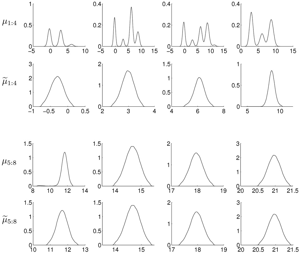
The first example uses synthetic data from a simple univariate example in Yao and Lindsay (2009), drawing n = 400 observations from $g(x|\mathrm{\Theta })={\displaystyle {\sum }_{j=1}^{8}0.125N({\mu }_j,1)}$ with μ_j = 3 * (j − 1) for j = 1 : 8. After a long run for burn-in of the MCMC, several EM solutions were identified by running iterative posterior mode searches from the MCMC parameters at every 1,000 iterates. The highest posterior mode so identified defined Θ^R. This reference point was also used as a starting point for 100,000 MCMC iterates, resulting in the summaries in Figure 1. We can see that there is a good deal of label switching in the marginal posterior density estimates based on the raw MCMC output, while those under relabeling are all unimodal and capture the true values.

Figure 1.

Plots of estimated marginal posterior densities for the component mean in the 8–component univariate mixture, simulated data example. Plots for μ_1:8 show results based on the raw MCMC samples, clearly and strongly evidencing the label switching issues via multimodal margins. Plots for μ̃_1:8 show results under the relabeling strategy, resulting in unambiguous and accurate (since the ground-truth is known in this synthetic example) identification of posteriors.

Further evaluations show performance similar to the preceding approaches of Stephens (2000) and Yao and Lindsay (2009) in this simple setting. It is worth repeating that the computations are substantially more burdensome in these earlier approaches, even in this “low p; low k, low n” context.

4.2 Flow Cytometry Example

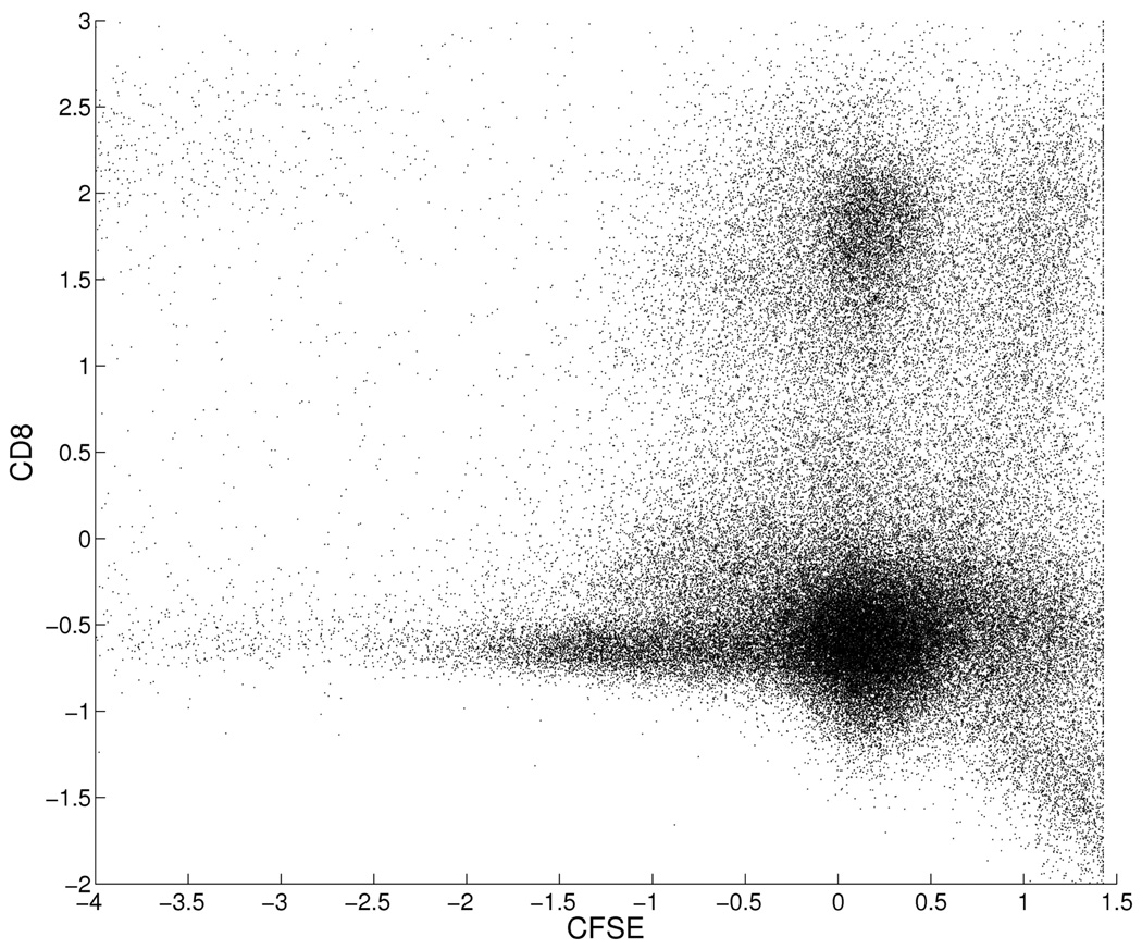
The second example uses a subset of flow cytometry data from Suchard et al. (2010). The applied context being one of identifying sub-populations in distributions of several cell surface proteins (Boedigheimer and Ferbas, 2008; Chan et al., 2008). We selected p = 2 marker proteins on n ≈ 100,000 cells from that immune response assay data set, choosing proteins CD8 and CDSE that are often critically relevant in identifying functional subtypes of immune cells. The scatter plot of measured levels in Figure 2 shows evidence of subtypes of cells with expected non-normal scatter within subtype. The applied strategy is that of fitting an encompassing normal mixture model and then grouping subsets of normal components to define subtypes (Chan et al., 2008; Lin et al., 2010). Dealing adequately with label switching is critical to this enterprise.

Figure 2.

Flow cytometry data on standardized levels of proteins CFSE and CD8

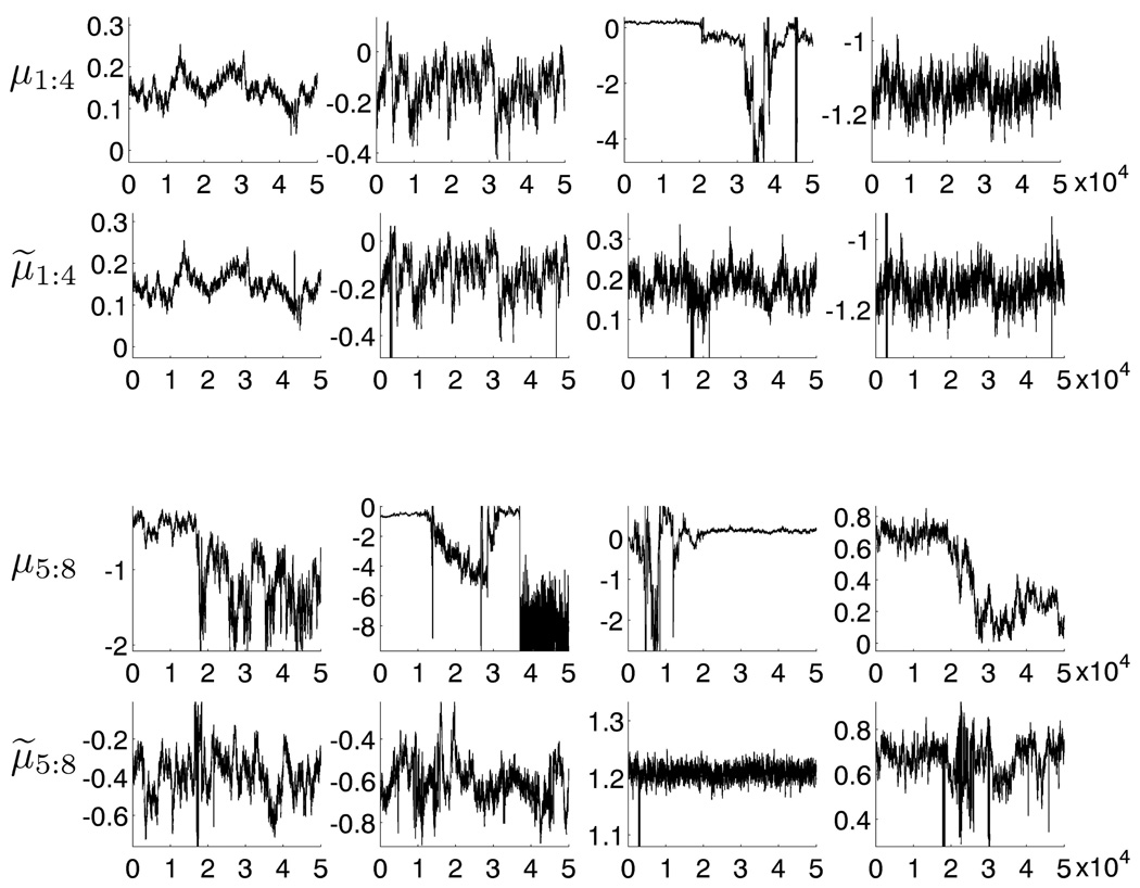
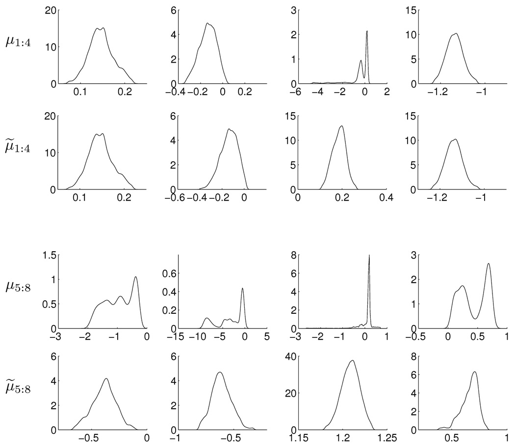
The mixture model uses a truncated Dirichlet process prior with an encompassing k = 32 components; the prior structure allows for fewer than this upper bound k to be represented in the data reflecting the use of these models to automatically cut-back to fewer components (e.g. Escobar and West, 1995; MacEachern and Müller, 1998a,b; Ishwaran and James, 2001; Chan et al., 2008; Ji et al., 2009). As in the previous example, the Gibbs sampler was run for thousands of iterations to ensure convergence; this was followed by many local searches using Bayesian EM to identify local posterior modes and so fix a reference Θ^R as the highest posterior mode so identified. Initializing at this set of parameters, we then ran the Gibbs sampler to identify and save a posterior sample of size 50,000. Figure 3 shows trace plots for the means of 8 (of the 32 components) on the CFSE dimension, with these 8 components selected according to their EM summary starting points. Figure 4 shows the corresponding estimates of marginal posterior densities for both the raw MCMC results and for the relabeled results.

Figure 3.

Trace plots of 8 component means in the CFSE dimension of the flow cytometry example. Plots for μ_1:8 are raw Gibbs sampler output and μ̃_1:8 the relabeled outputs.

Figure 4.

Marginal density estimates for 8 component means in the CFSE dimension of the flow cytometry example, based on raw (μ_1:8) and relabeled (μ̃_1:8) MCMC outputs.

4.3 Compute Time Benchmarks and Higher Dimensions

Computational efficiency and ability to scale with the number of mixture components k and, critically, the sample size n is a major concern. Investigations of this explored analyses in several contexts with data randomly sub-sampled from the above flow cytometry data set for realism. The C++ code is available stand-alone as well as integrated with the Duke CDP software for MCMC and Bayesian EM in truncated Dirichlet process mixture models (among other models)(Suchard et al., 2010). The test machine used was configured with a CPU (Intel Core i7-975 Extreme Quad-Core 3.33 GHz Processor) and GPU (Nvidia GTX 285 graphics card), and the software used core code in C++ and CUDA.

The example data set is in p = 15 dimensions. The number of observations and components analyzed were varied as in Table 1 that also summarizes running time results.

Table 1.

A simulation study to illustrate the percent computation time occupied by the relabeling algorithm for 1000 iterations of MCMC using a C++ extension of efficient CPU/GPU code for Bayesian analysis of truncated Dirichlet process mixture models (Suchard et al., 2010). This example uses data in p = 15 dimensions and examines running times for numbers of components k and sample sizes n that range across practically relevant values. All times are in seconds (real time).

n	k	Total Time	Relabeling	%
104	32	28.03	0.29	1.04
	64	53.83	1.46	2.71
	128	114.9	10.28	8.94
	256	287.4	78.87	27.4
105	32	77.82	0.94	1.21
	64	118.01	2.10	1.78
	128	206.80	10.93	5.28
	256	452.09	79.59	17.6
106	32	511.97	7.23	1.41
	64	734.13	8.29	1.13
	128	1156.16	17.16	1.48
	256	2100.11	85.78	4.08

5 Further Comments

A number of other examples and studies bear out the results exemplified above. This classificationbased relabeling strategy has the ability to perform as or better than existing methods with major computational advantages, and an ability to move beyond the very modest dimensions (p, k, n) that prior methods can address at all. As data sets increase in size and complexity, use of mixture models for sub-structure identification is increasing, and having effective, automatic relabeling is fundamental to practical utility. We have provided efficient code to enable interested readers to explore and evaluate the method presented and expect that it will find broad utility.

No method of relabeling will work wholly and consistently well. Overlapping components, that may be overlapping in a subset of the p dimensions, bedevil any method of addressing the inherent identification problem. The realization of label switching is increasingly hard to diagnose as p increases, and looking at marginal dimensions under one or more relabeling methods can mask the realities of random label switches in higher dimensions. Low probability components, sometimes “real” and of key applied interest (e.g. Manolopolou et al., 2010), though sometimes simply reflecting noise, can exacerbate the problem. One area of future potential development is to explore Yao and Lindsay’s idea of identifying with multiple posterior modes integrated with classification-based ideas. Perhaps more immediately, since the method here is computationally cheap, using several reference summaries would not be too costly and offers additional opportunity to dissect and resolve labeling identification ambiguities. The approach is also general with respect to component distributional form; the underlying ideas and strategy can be applied to more complex mixtures with hierarchical structure as well as non-normal and mixed components.

References

- Boedigheimer MJ, Ferbas J. Mixture modeling approach to flow cytometry data. Cytometry A. 2008;73:421–429. doi: 10.1002/cyto.a.20553. [DOI] [PubMed] [Google Scholar]
- Chan C, Feng F, West M, Kepler TB. Statistical mixture modelling for cell subtype identification in flow cytometry. Cytometry A. 2008;73:693–701. doi: 10.1002/cyto.a.20583. [DOI] [PMC free article] [PubMed] [Google Scholar]
- Escobar MD, West M. Bayesian density estimation and inference using mixtures. Journal of the American Statistical Association. 1995;90:577–588. [Google Scholar]
- Ishwaran H, James L. Gibbs sampling methods for stick-breaking priors. Journal of the American Statistical Association. 2001;96:161–173. [Google Scholar]
- Jasra A, Holmes CC, Stephens DA. MCMC and the label switching problem in Bayesian mixture models. Statistical Science. 2005;20:50–67. [Google Scholar]
- Ji C, Merl D, Kepler TB, West M. Spatial mixture modelling for unobserved point processes: Application to immunofluorescence histology. Bayesian Analysis. 2009;4:297–316. doi: 10.1214/09-ba411. [DOI] [PMC free article] [PubMed] [Google Scholar]
- Lau JW, Green PJ. Bayesian model based clustering procedures. Journal of Computational and Graphical Statistics. 2006;12:351–357. [Google Scholar]
- Lavine M, West M. A Bayesian method for classification and discrimination. Canadian Journal of Statistics. 1992;20:451–461. [Google Scholar]
- Lin L, Chan C, West M. Discussion Paper 10–23. Department of Statistical Science, Duke University; 2010. Discriminative information analysis in mixture modelling. Submitted for publication. [Google Scholar]
- MacEachern SN, Müller P. Computational methods for mixture of Dirichlet process models. In: Dey D, Müller P, Sinha D, editors. Practical Nonparametric and Semiparametric Bayesian Statistics. Springer-Verlag; 1998a. pp. 23–44. [Google Scholar]
- MacEachern SN, Müller P. Estimating mixture of Dirichlet process models. Journal of Computational and Graphical Statistics. 1998b;7:223–238. [Google Scholar]
- Manolopolou I, Chan C, West M. Selection sampling from large data sets for targeted inference in mixture modeling (with discussion) Bayesian Analysis. 2010;5:429–450. [PMC free article] [PubMed] [Google Scholar]
- Munkres J. Algorithms for the assignment and transportation problems. Journal of the Society of Industrial and Applied Mathematics. 1957;5:32–38. [Google Scholar]
- Stephens M. Dealing with label switching in mixture models. Journal of the Royal Statistical Society, Series B. 2000;62:795–809. [Google Scholar]
- Suchard MA, Wang Q, Chan C, Frelinger J, Cron AJ, West M. Understanding GPU programming for statistical computation: Studies in massively parallel massive mixtures. Journal of Computational and Graphical Statistics. 2010;19:419–438. doi: 10.1198/jcgs.2010.10016. [DOI] [PMC free article] [PubMed] [Google Scholar]
- West M. Hierarchical mixture models in neurological transmission analysis. Journal of the American Statistical Association. 1997;92:587–606. [Google Scholar]
- Yao W, Lindsay BG. Bayesian mixture labeling by highest posterior density. Journal of the American Statistical Society. 2009;104:758–767. [Google Scholar]