Same or Different? A Neural Circuit Mechanism of Similarity-Based Pattern Match Decision Making

Abstract

The ability to judge whether sensory stimuli match an internally represented pattern is central to many brain functions. To elucidate the underlying mechanism, we developed a neural circuit model for match/nonmatch decision making. At the core of this model is a “comparison circuit” consisting of two distinct neural populations: match enhancement cells show higher firing response for a match than a nonmatch to the target pattern, and match suppression cells exhibit the opposite trend. We propose that these two neural pools emerge from inhibition-dominated recurrent dynamics and heterogeneous top–down excitation from a working memory circuit. A downstream system learns, through plastic synapses, to extract the necessary information to make match/nonmatch decisions. The model accounts for key physiological observations from behaving monkeys in delayed match-to-sample experiments, including tasks that require more than simple feature match (e.g., when BB in ABBA sequence must be ignored). A testable prediction is that magnitudes of match enhancement and suppression neural signals are parametrically tuned to the similarity between compared patterns. Furthermore, the same neural signals from the comparison circuit can be used differently in the decision process for different stimulus statistics or tasks; reward-dependent synaptic plasticity enables decision neurons to flexibly adjust the readout scheme to task demands, whereby the most informative neural signals have the highest impact on the decision.

Introduction

Perception and cognition often require us to evaluate similarity of two sensory events and to judge whether they are the same or different. “Same versus different” comparison is a generic neural computation involved in a wide range of brain functions. For example, searching for an object in a crowded scene requires us to judge whether a currently viewed object matches an internal representation of the target object. Furthermore, mismatch between expected and experienced stimuli is believed to give rise to “prediction error” signals [e.g., in the forward model for motor learning (Wolpert and Miall, 1996)]. Match/nonmatch comparison between the environment and expectation has also been proposed to gate the entry of information into the long-term memory (Lisman and Grace, 2005; Kumaran and Maguire, 2007).

Match/nonmatch computation is often thought of as a decision on whether the difference between two signals is zero (match). However, recent experimental findings in delayed match-to-sample (DMS) tasks suggest a different view. In a DMS task, subjects are presented with a sequence of stimuli separated by delays, and a behavioral response is required if the current test stimulus is the same (match) as a previously shown sample stimulus. Intriguingly, converging evidence from physiological studies with behaving monkeys and human brain imaging (Turk-Browne et al., 2007; Duncan et al., 2009) pointed to two candidate neural mechanisms involved in match versus nonmatch computation. One is referred to as repetition suppression, a passive reduction of neural response to any stimulus repetition regardless of behavioral relevance (see Fig. 1C). Repetition suppression is the predominant neural signal observed in standard DMS tasks (see Fig. 1B) when the matching test is the only stimulus repetition within a trial (Miller et al., 1991, 1993; Miller and Desimone, 1994; Steinmetz and Constantinidis, 1995; Constantinidis and Steinmetz, 2001; Zaksas and Pasternak, 2006). The other is referred to as match enhancement, an active mechanism that is engaged whenever feature matching is not sufficient to perform a task, as for example when nonmatch can also be repetitive (e.g., ABBA) (see Fig. 1B), and irrelevant repetitions of nonmatch stimuli (BB) should be ignored. Neurophysiological recordings in the prefrontal (Miller et al., 1996; Freedman et al., 2003), temporal (Miller and Desimone, 1994), and parietal (Rawley and Constantinidis, 2010) cortices revealed two populations of neurons whose selectivity for visual stimuli is modulated by match/nonmatch context in complementary ways: match enhancement (ME) cells show higher firing response for a match than nonmatch to the sample, whereas match suppression (MS) cells exhibit the opposite trend (see Fig. 1D).

Figure 1.

Delayed match-to-sample task, neural encoding of match/nonmatch, and schematic of the circuit model. A, Left, Random dot stimulus. Right, The DMS task. The sample stimulus is followed by a sequence of test stimuli separated by delays. A behavioral response is required if the test matches the sample. B, Example trials in two versions of the DMS task. In the standard task, all intervening nonmatches are different, and the match is the only perceptual stimulus repetition within a trial. In the ABBA task, irrelevant repetitions of nonmatches should be ignored. C, Repetition suppression in inferior temporal cortex neurons in the standard DMS task [data from Miller et al. (1993)]. Average responses across cells to the same set of stimuli appearing as a sample, match, and nonmatch. D, Match enhancement and match suppression in two complementary populations of prefrontal cortex neurons in the ABBA task [data from Miller et al. (1996)]. Average responses across cells to the same set of stimuli appearing as a sample, match, nonmatch, and repeated nonmatch. E, Schematic of the circuit model. Neurons in the WM and comparison networks (ME and MS subpopulations) are tuned to directions of motion (indicated by arrows) and receive directional bottom–up input. Top–down projections from the WM to the comparison network are heterogeneous. ME neurons (red circles) receive stronger top–down excitation than MS neurons (blue circles). The decision network (match and nonmatch subpopulations) generates categorical match versus nonmatch choices by pooling activities of the ME and MS neurons through synapses that undergo reward-dependent Hebbian plasticity.

These observations raised a number of questions: (1) what are the network mechanisms for generating match enhancement and suppression neural signals, (2) how does the brain switch between the active and passive modes of computation, and (3) are enhancement and suppression neural signals sufficient to make same versus different decisions, and if so, how? Here, we examine possible answers to these questions by proposing a biophysically based circuit model that can learn and perform a DMS task in its entirety.

Materials and Methods

For the sake of concreteness, model simulations were performed with a DMS task in which the stimulus feature is the direction of motion in a field of moving dots (see Fig. 1A). Using the motion direction stimuli has three main advantages. First, the angle separation between any two motion directions is an analog quantity that objectively measures their similarity. Parametrical variation of the angle between the sample and test directions allows us to make quantitative predictions about neural encoding of similarity. Second, in the primates, processing of motion directions depends on neural activity in the cortical area MT, where most cells have bell-shaped tuning functions for the direction of motion (Dubner and Zeki, 1971; Britten et al., 1992; Born and Bradley, 2005). The encoding of motion directions by MT neurons is understood fairly well and can be captured with recurrent neural network models. Finally, the behavioral consequences of task difficulty for learning and performance can be studied by varying the fraction of test stimuli that are similar (less discriminable) to the sample. Although in this paper we focus on motion directions, all presented computational principles are generic and can be applied to other types of stimulus patterns.

Description of the model.

The model consists of three interconnected subsystems: the working memory (WM), comparison, and decision networks. All three are strongly recurrent networks with dynamics governed by local excitation and feedback inhibition (Compte et al., 2000; Wang, 2002; Wong and Wang, 2006). In simulations, we used a reduced firing-rate model that has been shown to reproduce neural activity of a full spiking neuron network (Wong and Wang, 2006). In this framework, the dynamics of each excitatory neural pool is described by a single variable s representing the fraction of activated NMDA conductance, and the neural firing rate is described as a function of the total synaptic current. The variable s is described by the following:

with γ = 0.641 and τ_s = 60 ms. The firing rate r is a function of the total synaptic current I (Abbott and Chance, 2005; Wong and Wang, 2006) as follows:

with a = 270 Hz/nA, b = 108 Hz, d = 0.154 s. The total synaptic current I consists of three main contributions: recurrent, sensory, and noisy, I = I_r + I_s + I_n. Recurrent input to a neuron i in the population A originating from the population B reads as follows:

where g_ij^B→A is a synaptic coupling between the neuron j in the population B and the neuron i in the population A.

Neurons in the WM and comparison networks are spatially organized and labeled by their preferred direction of motion θ_i (from 0° to 360°). Each population (WM, ME, and MS) was simulated by 256 discrete units s_i (i = 1 … 256) with equally spaced preferred directions (θ_i+1 − θ_i = 360°/256). Within each network, the synaptic couplings g_ij between neurons with preferred directions θ_i and θ_j have a Gaussian profile as follows:

with σ = 43.2°. Parameters J₋ and J₊ determine the amount of the recurrent inhibition and excitation in the circuit. The WM network can sustain persistent firing by reverberating activity because of strong recurrent excitation (J₊^WM = 2.2 nA, J₋^WM = −0.5 nA). In Figure 6, the peak location of persistent activity pattern was characterized by a population vector (Compte et al., 2000).

Figure 6.

Degradation of performance in the DMS task with memory delay. A, Memory of the sample is encoded by the peak location of the bell-shaped persistent activity pattern in the WM circuit (see Materials and Methods). Variance of the remembered sample growths linearly with time, consistent with a diffusion process. The insets show the probability density for the remembered sample after 1 s (orange) and 10 s (blue) delays (gray histogram, simulations; solid color line, Gaussian fit). B, Example traces for the peak location of the persistent activity pattern in the WM circuit, which represents the sample memory during the delay. C, Psychometric function in the DMS task for different durations of the memory delay. D, Psychometric threshold increases and the slope of the psychometric function decreases for longer delays. The overall performance decreases for longer delays but remains at relatively high level for all delays. Relative discrimination (ratio of the threshold at 0.2 s delay to the threshold at longer delays) decreases with the delay duration, which accounts for the psychophysical observations with monkeys (Pasternak and Greenlee, 2005). Stimulus statistics is the same as in Figure 7 for p₀ = 0.5.

The comparison network has match enhancement and suppression (ME and MS) neurons defined by heterogeneous top–down inputs. One subpopulation (ME neurons) receives excitation from the WM circuit with the Gaussian profile as in Equation 4 and σ = 43.2°, J₋^WM→ME = 0 nA, J₊^WM→ME = 1.15 nA. The rest of the comparison network are MS neurons that do not receive any top–down input J₋^WM→MS = J₊^WM→MS = 0 nA. We assume that excitatory conductances of the ME cells are weakened by a factor α = 0.975 because of a homeostatic mechanism acting to compensate for the top–down excitation in these cells. This homeostatic mechanism is operating on a very slow timescale, so that the value of α is held constant in all simulations. The comparison network is strongly dominated by inhibition with J₋ = −8.5 nA, J₊^MS→MS = J₊^ME→MS = 0.4 nA and J₊^ME→ME = J₊^MS→ME = αJ₊^MS→MS.

When a motion direction stimulus θ_s is presented, neurons in the WM and comparison networks receive sensory currents that depend on the preferred direction θ of the neuron as follows:

where σ_s = 43.2°, g_s^WM = 0.02 nA, g_s^MS = 0.13 nA, and g_s^ME = αg_s^MS. We assume that sensory signals reach the WM circuit only when attention is directed to store the sample in the WM. Signals form the test stimuli, as well as from the sample in the passive condition (simulating the repetition suppression) do not reach the WM circuit. In all simulations, sensory stimuli were presented for 0.6 s and separated by 1 s delay (except for the results in Fig. 6).

Noisy current replicates background synaptic inputs and obeys: τ_ndI_n/dt = − (I_n − I₀) + $\sqrt{{\tau }_n}{\sigma }_n\eta \left(t\right)$, where η(t) is a white Gaussian noise, I₀^MS = 3.1 nA, I₀^ME = αI₀^MS, I₀^WM = 0.3297, τ_n = 2 ms, and σ_n = 0.009 nA. For the results in Figure 6, the noise variance in the WM circuit was increased to σ_n^WM = 0.16 nA.

The ME and MS neurons have an additional current I_a mimicking the spike rate adaptation as follows: I^{ME,MS} = I_r + I_s + I_n + I_a, whereby I_a = g_as_a and g_a = 0.003 nA. The dynamics of s_a follows ds_a/dt = −s_a/τ_a + r, with τ_a = 10 s. We used a phenomenological model for the adaptation current, since our aim was to explore interactions between the passive and active memory mechanisms rather than to capture the precise biophysical mechanism of adaptation.

The strength of the top–down connections J₊^WM→ME and the homeostatic scaling parameter α were chosen so as to (1) achieve approximately equal responses in the ME cells to the preferred match and in the MS cells to the preferred nonmatch stimulus, and (2) replicate the experimentally observed difference in response to the match and nonmatch stimuli in the MS cells (see Fig. 1D). The magnitude of the adaptation current g_a was adjusted to mimic the experimental pattern of the passive repetition suppression in the MS cells (see Fig. 1C). Other observed firing rate patterns in the comparison network (as discussed in Results) were not purposely tuned.

The activities of the ME and MS neurons are pooled by the decision circuit with two competing neural populations selective for choice “match” and “nonmatch” (see Fig. 1E). When stimulated, activities of the two populations diverge according to winner-take-all dynamics, and the decision of the model is determined by the population with a higher activity. Across trials, the stochastic choice behavior of the decision circuit is characterized by a sigmoidal dependence of the probability P^M to choose match on the difference ΔI in synaptic input currents to the match and nonmatch pools (Soltani and Wang, 2006):

We used β = 200 nA⁻¹.

Plasticity rule.

The synapses connecting comparison neurons with the decision neurons are plastic. Each pair of presynaptic and postsynaptic cells is connected by a set of binary synapses that are in either a potentiated or a depressed state. The fraction c_pre^post of synapses in the potentiated state quantifies the strength of synaptic connection. Input currents to the match and nonmatch populations are expressed through the synaptic strengths as I^{M,NM} = gΣ_ic_i^{M,NM}r_i, where the sum goes through all neurons in the comparison network, r_i are their firing rates, and g = 1 nA/Hz.

At the end of each trial, all synapses onto the chosen population (match or nonmatch) are updated according to a reward-dependent Hebbian plasticity rule. If the choice of the model is rewarded, the synapses are potentiated [i.e., the synapses in the depressed state make a transition to the potentiated state with the rate q₀ · q(r) referred to as the learning rate (Fusi, 2002)] as follows:

If the choice of the model is not rewarded, the synapses are depressed as follows:

The maximal learning rate q₀ determines the speed of learning. The learning rate gradually depends on the presynaptic firing rate: q(r) = (1 + exp(−(r − r₀)/σ_q))⁻¹. We used r₀ = 15 Hz and σ_q = 4 Hz. For the results in Figure 9, we used q₀ = 10⁻³.

Figure 9.

Synaptic plasticity adjusts the readout scheme according to task demands, illustrated by simulations of a fine motion discrimination (Purushothaman and Bradley, 2005). Sample moves in the fixed reference direction. Test stimuli are inclined by Δθ = {±0.5°, ±1° … ±3°} relative to the reference direction. The task is to judge whether a test stimulus is inclined clockwise (Δθ > 0) or counterclockwise (Δθ < 0) relative to the reference. After learning, the choice-selective populations in the decision circuit encode clockwise/counterclockwise (instead of match/nonmatch) decisions and hence are labeled as CW and CCW. A, Spatiotemporal dynamics of the synaptic strengths. Differences of the synaptic strengths Δc = c^CW − c^CCW are color coded for comparison neurons with all preferred directions. x-axis, Trial number; y-axis, presynaptic neurons labeled by their preferred directions. Through learning, a connectivity profile emerges, such that neurons tuned clockwise and counterclockwise relative to the reference preferentially target the CW- and CCW-selective populations, respectively. B, Psychometric function for the fine motion discrimination. Psychometric threshold is ∼1°–2°. C, D, Strengths of synaptic connections to the CW-selective (red; c_ME^CW and c_MS^CW) and CCW-selective (blue; c_ME^CCW and c_MS^CCW) populations after learning. Activity of each neuron is gradually weighted in the decision process, whereby higher weights are assigned to the most sensitive neurons tuned 40°–70° away from the reference direction.

Simulations of the learning dynamics.

For modeling the learning process, it is computationally impractical to simulate the actual neural circuit (operating on the timescale of milliseconds) over thousands of trials. We devised the following approach to bypass this difficulty while faithfully capturing the behavior of the system. First, for the decision network, only the choice behavior but not the detailed temporal dynamics is important for learning. Therefore, on each trial, we evaluated the difference in the input currents ΔI, computed P^M using Equation 6, and then flipped a biased coin to determine the network choice on a single trial.

Second, we note that responses of the comparison neurons are not affected by learning, which only adjusts the readout scheme from these neurons. Therefore, to efficiently simulate the learning dynamics, we created a database of neural responses to different combinations of sample and test stimuli and used the database to investigate the learning process. Specifically, for each stimulus configuration, 100 trials of the model dynamics were simulated and stored in the database (except for 500 trials were simulated for the results in Fig. 6). Each trial in the simulations of the learning dynamics consisted of four sequential steps: (1) generate the sample and test motion directions according to the stimulus statistics; (2) choose one trial from the database that corresponds to the current sample and test directions; (3) evaluate the input currents to the decision circuit ΔI = gΣ_i(c_i^M − c_i^NM)r_i, and determine the network choice; (4) update synapses according to the learning rule. This approach is very efficient, since the database needs to be created only once, and then learning dynamics can be simulated for different stimulus statistics and different parameters of the plasticity rule using the same database.

The synaptic strengths were initialized with random values drawn from the uniform distribution on [0, 1]. After the learning dynamics reached a steady performance level, the psychometric function was obtained by averaging the model performance over 10⁶ trials (with ongoing learning).

Steady-state calculations of the model performance.

The synaptic strengths and model performance in the steady state can be calculated analytically. Let θ_s be the sample direction, which is uniformly distributed on [0°, 360°]. Possible directional differences, match θ₀ = 0° and nonmatch {θ_i ≠ 0°} (i = 1 … N), have the priors p₀ and {p_i}, respectively. The firing rates of neurons in the comparison network r_i(θ,θ_s) depend on the preferred direction θ, sample direction θ_s, and the directional difference θ_i of the neuron. Hence the learning rate of each neuron on every trial q[r_i(θ,θ_s)] also depends on θ, θ_s, and θ_i. Averaging the update rule Equations 7 and 8 over the sample direction results in the effective learning rate as follows:

The effective learning rate is different for ME and MS neurons because of difference in their firing rates, but it is the same for neurons with all preferred directions θ because of rotational symmetry of the ring architecture. Consequently, two sets of effective learning rates {q_i^ME} and {q_i^MS} determine the steady state of learning (index i refers to the directional difference θ_i).

Since the effective learning rate does not depend on θ, the steady-state values of synaptic strengths are also the same for neurons with all preferred directions. Hence, four synaptic strengths fully characterize the steady state as follows: c_ME^M, c_ME^NM, c_MS^M, c_MS^NM. The synaptic strengths of ME and MS neurons obey the same equations, but they differ because of different effective learning rates. The analytical expressions for the synaptic strengths are readily obtained as follows:

Here P_i^M denotes the probability to choose match when the ith directional difference is presented. The difference in synaptic strengths to the match and nonmatch populations Δc = c^M − c^NM determines the difference in the synaptic input currents ΔI_i = g[Δc_MEΣ_θr_i^ME(θ) + Δc_MSΣ_θr_i^MS(θ)], which in turn determines P_i^M. Hence Equations 9 and 10 have to be solved self-consistently, and we solve them numerically using the Levenberg–Marquardt algorithm.

Once the steady-state solution is obtained, P_i^M provides us the psychometric function. The overall performance (i.e., the overall fraction of correct responses) is then computed as follows: p₀P₀^M + Σ_i=1^N p_i(1 − P_i^M). The psychometric functions have sigmoidal shape and can be fitted with the function f(θ) = c/(1 + exp(b(θ − a))) of three parameters a, b, and c. The fitted value of cb/4 (measured in degrees⁻¹) is called the slope of the psychometric function and characterizes its steepness. The parameter c is the value of the psychometric function at 0° directional difference (i.e., represents the probability to correctly identify match). The psychometric threshold is defined as the sample-test directional difference at which the performance is 75% correct responses and is expressed through the fit parameters as a − b log(4c − 1).

In our model, the steady-state values of the synaptic strengths (Eqs. 9, 10) depend on the prior probabilities for match p₀ and nonmatch stimuli {p_i}. In this way, the model adjusts the behavioral output to various stimulus statistics, for example, when the match prior p₀ changes. Notably, the network model is not explicitly provided with the priors but learns them through experience.

Ideal Bayesian observer.

As a benchmark against which to evaluate the network performance, we consider an ideal observer that performs the task optimally using Bayesian inference. On each trial, the ideal observer makes a match versus nonmatch decision based on observed data x (e.g., the firing rate) and the knowledge of priors p₀, {p_i}. Let p(x|θ_i) denote the likelihood function of x when the directional difference θ_i is presented. The posterior distributions for match and nonmatch are computed using Bayes' rule:

where the denominator is p(x), and p(nonmatch|x) = 1 − p(match|x). These posterior distributions can be used to make a decision using one of several possible decision rules. For the strict Bayesian strategy, the alternative with the larger posterior is always selected; hence the probability to choose match equals the following:

For a probabilistic Bayesian strategy, the alternatives are chosen with probabilities equal to their posteriors; hence P(match choice|x) = p(match|x) in this case. The psychometric function P_i^M for the ideal observer is then computed for each directional difference θ_i by averaging P(match choice|x) over the probability to observe the data x:

We assumed that, on each trial, the observed data value is x = r(θ_i) + η, where r(θ_i) is the mean response when the directional difference θ_i is presented, and η is a Gaussian noise with zero mean and SD σ. Hence the likelihood p(x|θ_i) = ($\sqrt{2\pi \sigma }$)⁻¹exp(−(x − r(θ_i))²/(2σ²)). We considered two different choices for r(θ_i): (1) average firing rate of the ME population [r_ME(θ_i)] (see Fig. 3C, red line); (2) difference in the average firing rates of the ME and MS populations [r_ME(θ_i) − r_MS(θ_i)] (see Fig. 3C, red and blue lines). We also considered the case when x is a two-component vector with the mean {r_ME(θ_i), r_MS(θ_i)} and with two independent Gaussian noises. Performance of the ideal observer was very similar in all these cases and for both, strict Bayesian and probabilistic Bayesian, decision strategies.

Figure 3.

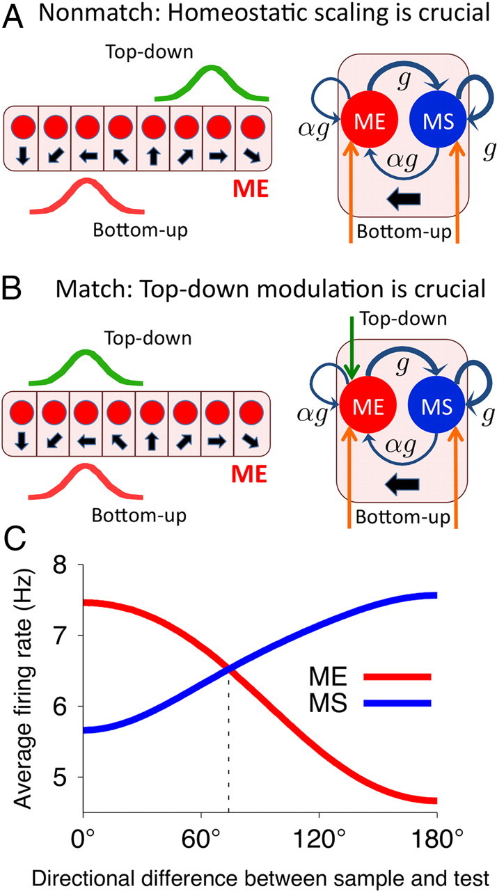
Circuit mechanism of match enhancement and suppression and neural tuning to the sample-test similarity. A, B, Left, Configuration of the top–down (green) and bottom–up (red) inputs to the ME population in the nonmatch (A) and match (B) conditions. Right, A column with the ME and MS neurons preferring the test stimulus is drawn. A, Nonmatch condition, The MS neuron has higher activity because of stronger recurrent excitation (thick blue arrows). B, Match condition, Top–down input compensates for weaker recurrent excitation, and the ME neuron has higher activity. C, Similarity tuning. Average population firing rate for the ME (red line) and MS (blue line) neurons as a function of directional difference between the sample and test. The ME and MS populations are parametrically tuned to the sample-test similarity in complementary ways.

For the comparison with the network model in Figure 7, we computed performance of the ideal observer using x as the difference in the average firing rates of the ME and MS populations and the strict Bayesian strategy. The noise SD σ was adjusted to approximately match the psychometric threshold and the overall performance for the network model and the ideal observer for p₀ = 0.5.

Figure 7.

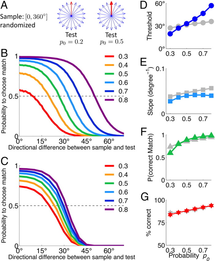
Plastic synapses encode priors for match and nonmatch and act to optimize performance. A, Schematic of the stimulus statistics in the DMS task with different priors for match. Sample motion direction is drawn from a uniform distribution on [0°, 360°]. Match (red arrow) corresponds to zero directional difference. Nonmatches (blue arrows) differ from the sample by Δθ = {±5°, ±10° … ±180°}, which are all equally probable. Note that the smallest nonmatch directional difference is ±5°, which sets the tolerance level. Match and nonmatch trials are randomly interleaved. Prior probability for a match trial is p₀ (indicated by the thickness of the red arrow). B, Performance of the network model for different match priors p₀ (colored lines labeled by p₀ values). C, Performance of the ideal Bayesian observer for different match priors p₀. In both cases (B, C), the psychometric function changes toward higher probability to choose match as p₀ increases, which reflects the trade-off involved in fine discrimination between the match and nonmatch stimuli that are similar to the sample. D–G, Psychometric threshold (D), slope of the psychometric function (E), probability to correctly identify match (F), and the overall performance (G) for the network model (colored symbols) and for the ideal Bayesian observer (gray symbols) as functions of the match prior p₀. Although changes in the psychometric function of the network model differ quantitatively from the Bayesian strategy, the overall performance of the network is virtually the same as for the ideal Bayesian observer.

Alternative model.

In the core of our model (see Fig. 10A, two-pool comparison model) are two neural populations, ME and MS neurons, that perform the comparison computation and exhibit complementary tuning to the sample test similarity (see Fig. 3C). We have also considered an alternative model based on simple addition of two signals: sensory input from the test stimulus and WM input representing a stored sample. The addition computation can be performed by a single neural population with converging sensory and WM inputs (see Fig. 10A, one-pool addition model). We implemented the one-pool addition model similarly to our two-pool model; however, instead of heterogeneous (ME and MS) comparison population, the one-pool model has a single “addition population” that receives sensory and WM inputs. All neurons in the addition population receive excitation from the WM circuit with the Gaussian profile as in Equation 4 and J₊ = 1.15 nA and J₋ = 0 nA. Since the top–down excitation is homogeneous, there is no heterogeneity in the strengths of recurrent connections, bottom–up inputs and background noisy currents within the addition population. For all cells, we set g_s = 0.13 nA, I₀ = 3.1 nA, and the recurrent connections follow the Gaussian profile (Eq. 4) with J₊ = 0.4 nA and J₋ = −8.5 nA. Other parameters are the same as in the two-pool model.

Figure 10.

Behavioral performance in the two-pool comparison model, but not in the one-pool addition model, is robust to changes in the sensory input strength. A, Schematics of the two-pool comparison model (simplified version of Fig. 1E) and of the one-pool addition model (for details, see Materials and Methods). B, Average population firing rate for the ME (solid line) and MS (dashed line) neurons in the two-pool model as a function of directional difference between the sample and test. Black line, Control; gray line, doubled sensory input strength. The difference in the activity of ME and MS neurons is only slightly affected by the increase in the input strengths, whereas the firing rates in both populations increase significantly. C, Average population firing rate for the addition population in the one-pool model as a function of directional difference between the sample and test. Black line, Control; gray line, doubled sensory input strength. The black dashed line indicates the firing rate threshold for match versus nonmatch decisions, obtained by fitting the parameters of the readout (Eq. 14) so as to match the psychometric functions for the one- and two-pool models in the control condition. D, In the two-pool model, the psychometric threshold and overall performance remain almost the same for the control (black bar) and doubled (gray bar) input strength. In the one-pool model, the overall performance decreases and the psychometric threshold increases with the input strength. For the doubled input strengths (gray bar), performance drops to the chance level (dashed line), and the psychometric threshold (defined at 75% correct performance) cannot be determined; for comparison purpose, we plot the maximum possible threshold value, 180°.

In the one-pool model, larger overlap between the top–down and bottom–up inputs leads to higher overall activity in the addition population. As a result, the average firing rate in the addition population gradually decreases with directional difference between the sample and test, resembling similarity tuning of the ME neurons in the two-pool model (see Fig. 10B,C, solid black lines). Match/nonmatch decisions can be read out from the single addition population by a simple threshold mechanism. Specifically, we assumed that the probability of the match decision is given by a sigmoidal function as follows:

where r is the averaged firing rate in the addition population, r_th is the firing-rate threshold, and parameter σ_r determines precision of the readout system.

To illustrate differences in behavioral performance of the one- and two-pool models, we asked how robust is the performance of each model to changes in the input strength (e.g., because of change in the contrast of visual stimuli) (see Fig. 10A,B). To this end, we simulated neural activity in both models in response to test stimuli with control (g_s = 0.13 nA) and doubled (g_s = 0.26 nA) strength. For fair comparison, with the control stimulus strength, the parameters r_th and σ_r in Equation 14 for the one-pool model were adjusted such that the psychometric function matches for the two models. With the doubled stimulus strength, the performance of both models was tested with the parameters of the readout systems fixed at the values obtained for the control stimulus strength.

Results

Computational hypotheses: building blocks of the circuit model

The model comprises three interconnected local circuits that correspond to three basic operations involved in the DMS task: the WM, comparison, and decision neural networks (Fig. 1E) (for details, see Materials and Methods). Neurons in the WM and comparison networks are tuned to motion directions and receive directional bottom–up inputs. The top–down projections from the WM circuit to the comparison network are excitatory and topographically organized: neurons with similar preferred directions are more strongly connected. Sample stimulus triggers persistent firing in the WM circuit, which represents a memory of the sample. This internal representation of the sample is maintained during the delay through reverberating neural activity (Camperi and Wang, 1998; Compte et al., 2000; Gutkin et al., 2001; Wang, 2001) and provides a top–down signal to modulate neural responses to test stimuli in the comparison network.

The core component of the model is the comparison network. Neurons in the comparison network respond differently to the test stimuli depending on whether they match the sample and in this way implement the comparison operation. The match/nonmatch sensitive modulations of responses arise from three simple biophysical ingredients. First, all cells in the comparison network are endowed with an adaptation current with a long time constant (∼10 s) (Sanchez-Vives et al., 2000; Wang et al., 2003; Pulver and Griffith, 2010). The spike rate adaptation leads to a diminished response to any repeated stimulus and thus captures passive repetition suppression. Second, the top–down projections from the WM circuit are topographically organized but naturally heterogeneous: just by chance different cells within each column receive different amount of top–down excitation. The cells that receive stronger top–down excitation (Fig. 1E, red) show active ME, and the cells that receive weaker top–down excitation (Fig. 1E, blue) show MS, as explained in the following section. Finally, homeostatic regulation of excitatory synapses (Turrigiano et al., 1998; Renart et al., 2003) acts to maintain the average firing rate in the network and to keep the overall amount of excitation approximately equal for all cells. As a result, the recurrent and bottom–up synapses on the ME cells are slightly weakened to compensate for the top–down excitation, compared with the MS cells. As we shall see, the difference in strength of recurrent connections in the ME and MS cells is crucial to generate enhanced responses to nonmatches in the MS cells. Note that the homeostatic mechanism is operating on a very slow timescale; hence in all simulations the difference in strength of recurrent connections in the ME and MS cells is held constant.

It is noteworthy that the model assumes that the ME and MS effects arise naturally from heterogeneous top–down excitation and inhibition-dominated recurrent dynamics in the comparison network, and no learning is involved in shaping responses of the ME and MS neurons. It is possible that different tasks may engage ME and MS cells differently. For instance, in a task in which working memory might not be necessary, the ME cells might not receive top–down inputs and therefore would show passive repetition suppression.

The activity of the ME and MS neurons is readout by a downstream decision network, modeled similarly as in the previous work (Wang, 2002; Wong and Wang, 2006), that generates categorical match versus nonmatch decisions. The decision network comprises two neural populations: match neurons (Fig. 1E, orange) and nonmatch neurons (Fig. 1E, purple) fire at higher rate for match and nonmatch decisions, respectively. Unlike the comparison neurons, which exhibit ME and MS as a modulation of their selectivity for motion direction, the decision neurons carry a pure decision (response) signal and are not selective to any stimulus feature. In addition, the decision neurons acquire their decision (response) preferences through learning. The synapses connecting the comparison and decision networks undergo reward-dependent Hebbian plasticity (Soltani and Wang, 2006, 2010; Fusi et al., 2007). We will show that learning ultimately generates connectivity profiles such that the activity of the ME and MS neurons can be read out differently by the decision network in a way that allows flexible mapping of comparison signals onto arbitrary motor response. The model is able to learn different variants of the DMS task using the same ME and MS signals, and to flexibly adjust the decision criteria when the stimulus statistics are changed.

In the model, we do not assign the working memory, comparison, and decision-making operations to specific brain areas. The local cortical circuits for these three basic operations may be located within a single brain area, or be distributed across several areas. For example, subpopulations of neurons in the prefrontal cortex exhibit activities consistent with all operations involved in the DMS task: sample-selective delay activity, ME/MS comparison signals, and match/nonmatch decision signals (Miller et al., 1996; Freedman et al., 2002). However, ME and MS neural signals have also been observed in the parietal areas 7a (Rawley and Constantinidis, 2010), LIP and MIP (Swaminathan et al., 2010), in the inferior temporal cortex (Miller and Desimone, 1994; Freedman et al., 2003), and in the area V4 (Kosai et al., 2010). These areas differ in the magnitude, latency, and the proportion of neurons carrying each type of signal. This suggests that they are playing distinct or complementary roles in the match/nonmatch decision making, but which area is the source of comparison and decision signals remains to be elucidated in the future.

Active and passive comparison mechanisms

We first consider the dynamics of the comparison network (Fig. 2). The top–down input modulates neural activities without disrupting selectivity for motion direction. Neurons respond to their preferred test stimuli, but the response is higher in the ME cells than in the MS cells if the sample was also the preferred stimulus (match), and vice versa if the sample was the antipreferred stimulus (nonmatch) (Fig. 2A–C). The ME and MS effects are specific for behavioral matches (i.e., for stimuli that match the sample stored in the WM circuit), as demonstrated by the responses to repeated nonmatch in Figure 2, A and C. The model thus reproduces the salient neural activity patterns observed in behaving monkeys (compare Figs. 2C, 1D). Interestingly, the model makes a testable prediction that the ME cells exhibit sample-selective delay activity (Fig. 2A,B). The delay activity in the ME neurons is induced solely by the top–down input, since the comparison network is dominated by recurrent inhibition and cannot sustain persistent firing on its own.

Figure 2.

Active and passive memory mechanisms in the circuit model: active match enhancement and suppression (A–C), passive repetition suppression (D–F). A, D, Spatiotemporal activity pattern in the WM, ME, and MS populations in an ABBA task, where a sample (90°) is followed by two nonmatch test stimuli (270°) and then by the final match (90°). x-axis, Time; y-axis, neurons labeled by their preferred directions; firing rate is color-coded. A, Comparison neurons respond to their preferred stimuli, but the activity is higher in the ME cells than in the MS cells for the match, and vice versa for the nonmatch stimuli. D, If the activity in the WM circuit is disrupted, passive repetition suppression prevails in the comparison neurons. B, E, Firing rates of a neuron preferring the test stimulus on two trials: when the test appears as a match (orange line) and as a nonmatch (purple line). In the match condition, the sample is also the preferred stimulus for this neuron, and in the nonmatch condition the sample is the antipreferred stimulus. Note sample-selective persistent activity in the ME cell during the delay. C, F, Average responses to the preferred stimulus of the neuron appearing as a sample, match, nonmatch, and repeated nonmatch. These model results account for the single-neuron activities recorded from behaving monkeys in Figure 1, C and D.

If the sample-tuned modulation from the WM circuit is disrupted (e.g., if the sample stimulus does not trigger persistent firing or if the top–down connections are absent), the active mechanism is abolished and the passive repetition suppression prevails in all cells in the comparison network (Fig. 2D–F; compare with experimental data in Fig. 1C). The passive mechanism does not distinguish behaviorally relevant and irrelevant repetitions; hence responses to match and repeated nonmatch are equally suppressed.

The circuit mechanism of active enhancement and suppression is illustrated in Figure 3, A and B. In the nonmatch condition (Fig. 3A), the bottom–up and top–down inputs target different columns in the ME population. The neurons tuned to the test stimulus are effectively driven by the bottom–up and recurrent inputs only. In this case, the ME cells have lower activity than the MS cells, since the recurrent and bottom–up synapses are weaker in the ME cells. In the match condition (Fig. 3B), the bottom–up and top–down inputs converge to the neurons within the same column. In this case, the top–down input compensates for the weaker recurrent excitation in the ME cells as well as for the adaptation-induced reduction in their responsiveness. Consequently, the ME cells show higher activity than the MS cells.

The dynamics in the comparison network have to be strongly dominated by recurrent feedback inhibition to achieve that the response to match stimuli is lower in the MS cells than in the ME cells. Indeed, in the match condition, the total activity of the ME and MS cells, and hence the recurrent excitation to the MS cells (that have stronger recurrent synapses), is comparable with that in the nonmatch condition. Nevertheless, in the match condition, the MS cells show lower activity than in the nonmatch condition. This is possible if the overall feedback inhibition is higher in the match than in the nonmatch condition. Since the feedback inhibition is approximately proportional to the summed activities of the ME and MS neurons, a signature of this network mechanism is that the total activity of the ME and MS cells is slightly higher in the match than in the nonmatch condition. In other words, the response of the ME cells in the nonmatch condition is lower than the response of the MS cells in the match condition (Figs. 2C, 3C). Our proposed mechanism of enhancement and suppression hence accounts for some subtle details of the experimental data shown in Figure 1D. Notably, the overall activity in the comparison network is higher for match than for nonmatch stimuli despite the passive adaptation acting to reduce firing of the mostly active cells in the match condition.

When examining firing patterns in the comparison network, for all possible comparisons across different cell types and sample/match/nonmatch conditions, what matters the most is the difference in response of the ME and MS cells to the same test stimulus. This difference in firing of the ME and MS cells is what is used by the readout system to generate a categorical match versus nonmatch decision. The dynamical enhancement and suppression mechanisms in our model underlie this pattern of firing rate differences, which closely captures experimental data. In contrast, the exact responses to the sample in the ME and MS cells are not essential. In our model, neural responses to the sample are somewhat higher than the ME neural response to a nonmatch or MS response to a match test stimulus, which is attributable to the transient interplay of the rising activity in the WM circuit and of the building up adaptation current during the sample stimulus presentation as well as the enhanced global feedback inhibition afterward.

Sample-test similarity tuning in the ME and MS populations

So far, we considered only nonmatch stimuli that differed by 180° from the sample (i.e., the opposite direction of motion). It is interesting to see how the comparison network handles nonmatch stimuli with various degree of similarity to the sample. The directional difference between the sample and test determines the amount of overlap between the bottom–up and top–down inputs to the ME population (Fig. 3A). The larger this overlap is, the higher is the overall activity in the ME population. Accordingly, the response of the ME population is the highest in the match condition and gradually decreases with the directional difference, whereas the MS population exhibits the opposite pattern (Fig. 3C). In this way, neurons in the comparison network exhibit sigmoidal tuning to similarity between the sample and test, whereby activity of the ME cells increases and that of the MS cells decreases for more similar stimuli. Our model makes it explicit that similarity tuning is required to perform a DMS task and predicts that match enhancement and suppression effects are tuned to similarity in complementary ways. This predication can be tested experimentally.

Since a match/nonmatch decision is expected to rely on the differential signals from the ME and MS neurons, a key property of the network is the value of the directional difference at which the sample-test similarity tuning curves of the ME and MS cells cross. This value depends on the width of neural tuning in the WM and comparison networks, which is ∼30°–50°, comparable with those observed in cortical neurons (Albright, 1984). Consequently, the two similarity tuning functions are coarse, and the crossing point is at ∼70° (Fig. 3C, dashed vertical line). This raises two questions: Is the coarseness of the similarity tuning the main factor limiting the decision accuracy, and how can coarsely tuned neurons carry out fine discriminations? These questions are addressed in the following sections, in which we propose a downstream decision circuit that generates match/nonmatch choices based on activities of the ME and MS neurons.

Learning to compute the match/nonmatch decision

The decision circuit comprises two competing neural populations selective for the choices (e.g., match and nonmatch) (Fig. 1E) and exhibits winner-take-all dynamics. Across trials, the stochastic choice behavior in the decision circuit is characterized by a sigmoidal function, which represents how the probability of making a choice depends on the difference in synaptic input currents to the two competing neural populations (Soltani and Wang, 2006) (Fig. 4B). Since the ME and MS neurons are entangled within the comparison network and have the same cellular properties, it is reasonable to assume that the ME and MS neurons are all connected to both selective populations in the decision circuit. Specific connectivity profiles that differentially weight activities of the ME and MS neurons should emerge from experience-dependent learning (Fig. 4A).

Figure 4.

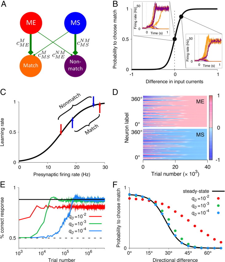
Learning the DMS task through reward-dependent Hebbian plasticity. A, Schematic of synaptic connections between the comparison (ME and MS) and the decision (match and nonmatch) populations. Through synaptic plasticity, a connectivity profile emerges such that the ME and MS neurons preferentially target match and nonmatch populations, respectively (i.e., Δc_ME = c_ME^M − c_ME^NM > 0 and Δc_MS = c_MS^M − c_MS^NM < 0). B, In the decision circuit, the trial-averaged performance is captured by the sigmoidal dependence of probability to choose match on the difference in synaptic input currents to the match and nonmatch populations, ΔI = gΣ_i[Δc_MEr_ME + Δc_MSr_MS]. Firing rates of the match (orange) and nonmatch (purple) populations in 10 simulated trials are shown in two cases: for ΔI = 0 when match and nonmatch are chosen equally often; for ΔI > 0 when match is chosen more frequently than nonmatch. C, Learning rate is a monotonically increasing function of the presynaptic firing rate. The arrows indicate the firing rates of a ME (red) and MS (blue) neuron in response to their preferred stimulus appearing as match and as nonmatch (0° and 180° directional difference, respectively). D, Spatiotemporal dynamics of the synaptic strengths. Differences of the synaptic strengths Δc_ME and Δc_MS are color coded for all comparison neurons. x-axis, Trial number; y-axis, presynaptic neurons labeled by their preferred directions. E, In the learning process, the fraction of correctly performed trials increases faster for higher learning rates q₀. Solid black line, Steady-state performance; dashed line, chance level. F, Psychometric function obtained from the steady-state calculations (black line) and from simulations with different q₀ (colored circles). The performance approaches the steady-state level for sufficiently low q₀. Stimulus statistics is the same as in Figure 7 for p₀ = 0.5.

We used a reward-dependent Hebbian learning rule similar to that in the previous work (Soltani and Wang, 2006, 2010; Fusi et al., 2007) (see Materials and Methods), but with the additional assumption that the synaptic potentiation/depression rate q₀ · q(r) is an increasing function of the presynaptic firing rate r (Fig. 4C). Since neurons in the decision circuit have binary (high or low) activities, for simplicity we reduce the dependence on the postsynaptic firing to a binary rule: only synapses onto the population with the high activity (i.e., for the winner that determines the choice) are updated. Synapses are potentiated in reward trials, and depressed in error trials.

Gradual dependence of q(r) on the presynaptic firing is the key to learning the task. Consider a ME cell and a MS cell preferring the test stimulus, and consider their four connections to the match and nonmatch populations, c_ME^M, c_ME^NM, c_MS^M, c_MS^NM (Fig. 4A). If the test stimulus is a match, then the firing rate and hence the amount of potentiation/depression is slightly higher for the ME cell (Fig. 4C). The match choice is rewarded in this condition and induces potentiation in both cells, but synapses from the ME cell are potentiated more than those from the MS cell (Fig. 4C), leading to c_ME^M > c_MS^M. The nonmatch choice is not rewarded in this condition, and synapses from the ME cell are depressed more than the synapses from the MS cell, leading to c_ME^NM < c_MS^NM. The similar argument applies to the case of a nonmatching test. In this way, learning eventually gives rise to a synaptic connectivity profile such that the ME and MS neurons preferentially target the match and nonmatch populations, respectively (Fig. 4A,D).

If learning is performed with randomized direction of the sample stimulus, all motion directions are presented equally often during the test. As a consequence, the steady-state synaptic strength for each comparison neuron is independent of its preferred motion direction. That is, four values, c_ME^M, c_ME^NM, c_MS^M, c_MS^NM, fully characterize the steady state of the learning process (Fig. 4D). The steady-state values of synaptic strengths can be calculated analytically (see Materials and Methods), which in turn allow us to calculate the psychometric function of the network (Fig. 4E,F). The steady-state prediction is the upper bound on the behavioral performance. Ongoing learning in the network produces time-varying fluctuations of synaptic strengths around their steady-state values, which results in slightly lowered performance. The magnitude of these fluctuations increases with the maximal learning rate q₀. There is therefore a trade-off between faster learning and higher accuracy (Fig. 4E,F). For sufficiently low q₀, the performance approaches the steady-state level.

What determines the behavioral performance

Behavioral performance in our model is jointly determined by three factors: firing rates of neurons in the comparison circuit, sensitivity of the decision circuit, and the profile of synaptic connections between the comparison and decision networks. To discern contributions from each of these three factors, we computed the performance of the model, allowing one of them to vary while holding the remaining two factors fixed (Fig. 5). It is instructive to perform this analysis using linear similarity tuning in the ME and MS populations as well as linear dependence of the learning rate q(r) on the firing rate, as we have assumed for the results in Figure 5. Linear similarity tuning allows us to determine and parametrically vary the sharpness of tuning through just a single parameter, the tuning slope α. Moreover, the slope α is the same for all directional differences and the accuracy at small directional differences is not constrained by the nonlinear saturation as it is the case for sigmoidal tuning.

Figure 5.

The behavioral performance of the model is jointly determined by the firing rates of the ME and MS neurons, sensitivity of the decision circuit, and the profile of synaptic connections between the comparison and decision circuits. For this simplified analysis, we assumed linear similarity tuning in the ME and MS populations as well as linear dependence of the learning rate q(r) on the firing rate. Specifically, we used the functions f_ME,MS(x) = ±αx + 0.5(1 ∓ α), where the upper and lower signs refer to the ME and MS populations, respectively. For different directional differences θ_i, the firing rates followed: r_ME,MS(θ_i/180°) = 12 Hz · f_ME,MS(x), and the learning rates were just q_ME,MS(θ_i/180°) = f_ME,MS(x). A, The parameter α determines the sharpness of similarity tuning in the ME (solid lines) and MS (dashed lines) populations, whereby larger α corresponds to larger difference between the activities of the ME and MS populations. B, The overall performance of the model (fraction of correct responses) color coded as a function of synaptic differences Δc_ME and Δc_MS. Right panel, Zoom into the region of small Δc. The white star indicates the steady-state Δc obtained through learning. α = 0.4 and β = 200 nA⁻¹ are fixed. C, Two contributions to the difference in postsynaptic currents, |ΔI_ME| (solid lines) and |ΔI_MS| (dashed line) for different values of λ = |Δc_MS/Δc_ME|. The crossing point of these two curves and hence the psychometric threshold shift to larger directional differences for λ < 1, and to smaller directional differences for λ > 1. α = 0.4. D, Dependence of the psychometric function on the sharpness of similarity tuning in the comparison network. Sharper tuning (corresponds to larger values of α) results in lower psychometric threshold, larger slope of the psychometric function, and better overall performance. β = 200 nA⁻¹ is fixed. E, Dependence of the psychometric function on the sensitivity of the decision network. Higher sensitivity (corresponds to larger values of β) results in lower psychometric threshold, larger slope of the psychometric function, and better overall performance. α = 0.4 is fixed. The synaptic strengths in D and E are adjusted through learning. Stimulus statistics is the same as in Figure 7 for p₀ = 0.5.

First, consider how the performance of the model depends on the synaptic connectivity profile, with the parameters of the comparison and decision networks fixed. In Figure 5B, we plot the overall performance of the model (percentage correct responses) as a function of differences in synaptic strengths Δc_ME = c_ME^M − c_ME^NM and Δc_MS = c_MS^M − c_MS^NM. The synaptic strengths in Figure 5B are not adjusted by learning, we rather ask how well does the model perform for given values of synaptic strengths. Note that −1 ≤ Δc ≤ 1, since the synapses are bounded 0 ≤ c ≤ 1.

Probability of choices in the decision circuit depends on the difference in input currents to the match and nonmatch selective populations, ΔI = g[Δc_MEr_ME + Δc_MSr_MS]. If both Δc_ME and Δc_MS have the same sign, which means that both ME and MS cells are more strongly connected to the same pool in the decision circuit, then ΔI has the same sign for all directional differences. In this case, the model always generates the same response and the performance is at chance level (Fig. 5B, green area). If Δc_ME < 0 and Δc_MS > 0, then the match response is more probable when the activity in the MS population is higher (i.e., for large directional differences) and less probable when the activity in the ME population is higher (i.e., for small directional differences). In this case, the performance is worse than chance (Fig. 5B, blue area). Finally, the region where Δc_ME > 0 and Δc_MS < 0 corresponds to the ME and MS cells being more strongly connected to the match and nonmatch populations, respectively. Here, the match response is more (less) probable for small (large) directional differences and the performance is higher than chance (Fig. 5B, yellow-to-red area).

Let us now see how within this region, where Δc_ME > 0 and Δc_MS < 0, the performance and the psychometric threshold of the model depend on the relative magnitudes of synaptic strengths, λ = |Δc_MS/Δc_ME|. In this region, the difference in synaptic currents can be rewritten as ΔI = |ΔI_ME| − |ΔI_MS|, where |ΔI_ME| = g|Δc_ME|r_ME and |ΔI_MS| = g|Δc_MS|r_MS. The dependence of these two contributions on the directional difference is obtained just by multiplying the similarity tuning curves of the ME and MS neurons by their respective |Δc| values (Fig. 5C). The directional difference at which |ΔI_ME|(θ_i) and |ΔI_MS|(θ_i) curves cross corresponds to ΔI = 0 [i.e., to P(match) = P(nonmatch) = 0.5] and is referred to as the point of subjective indifference (PSI). Let us see how PSI, and consequently the psychometric threshold, depend on the parameter λ. For λ = 1 (i.e., |Δc_MS| = |Δc_ME|), the two curves, |ΔI_ME|(θ_i) and |ΔI_MS|(θ_i), cross exactly at the same directional difference where r_ME(θ_i) and r_MS(θ_i) curves cross (Fig. 5C, orange lines). Since the similarity tuning in the ME and MS neurons is coarse, the PSI and the psychometric threshold are large (∼90°) in this case. For λ < 1 (i.e., |Δc_MS| < |Δc_ME|), the crossing point of |ΔI_ME|(θ_i) and |ΔI_MS|(θ_i) shifts to even larger directional differences (Fig. 5C, blue line). Hence the PSI and the psychometric threshold increase, which is reflected in lower overall performance (Fig. 5B, yellow off-diagonal area). In contrast, for λ > 1 (i.e., |Δc_MS| > |Δc_ME|), the crossing point of |ΔI_ME|(θ_i) and |ΔI_MS|(θ_i) shifts to smaller directional differences (Fig. 5C, green line). The PSI and the psychometric threshold decrease and the overall performance increases (Fig. 5B, dark-red off-diagonal area) until the imbalance between |Δc_ME| and |Δc_MS| reaches the value where |ΔI_ME| < |ΔI_MS| for all θ_i and the performance quickly drops to the chance level [the drop-off happens within the range of ΔI values in which the choices in the decision network are stochastic (Fig. 5B, right panel)]. The performance drops off sharply because of the discontinuity in the correct response: 0° is the match, but any nonzero directional difference is a nonmatch. As long as the curves |ΔI_ME|(θ_i) and |ΔI_MS|(θ_i) cross just between 0° and the smallest nonmatch directional difference ψ₁ (which is 5° in Fig. 5), the performance is the best possible, but a small change in the synaptic strengths resulting in |ΔI_ME|(0°) < |ΔI_MS|(0°) will cause the network to respond “nonmatch” to 0° directional difference and hence the chance level performance. Note that the reward-dependent learning naturally adjusts synaptic strengths (Fig. 5B, white star) and drives the network as close as possible to the best performance, but far enough from the drop-off boundary so that fluctuations of synaptic strengths do not result in the chance level performance.

Another overall trend is that the performance slightly improves for larger values of |Δc|. This is because larger Δc result in larger absolute values of ΔI, for which the choices of the decision network are less stochastic (Fig. 4B). For the parameters as in Figure 5B, the performance of ∼100% correct can be achieved with large enough |Δc|. How well does our learning rule perform compared with what is optimally possible? The steady-state values of Δc resulting from the learning rule (Fig. 5B, white star) correspond to 95% correct performance, which is slightly less than optimally possible. This is because the absolute values of learned Δc are small. These values reflect the difference in the average firing rate of a cell on rewarded match and nonmatch trials, and since the similarity tuning is smooth, the steady-state Δc are small.

The dependence of the behavioral performance of the model on sharpness of the similarity tuning (parameter α) and on sensitivity of the decision circuit (parameter β) is presented in Figure 5, D and E, respectively. Here, synaptic strengths are adjusted through learning using linear ME and MS tuning curves (Fig. 5A). Shallower similarity tuning as well more stochastic decision circuit have similar effect on the behavior, producing decrease in the overall performance, increase in the psychometric threshold, and decrease in the slope of the psychometric function.

Degradation of performance with memory delay

In working-memory tasks, performance accuracy is known to decay with the duration of the memory delay (Pasternak and Greenlee, 2005). We propose that the main cause of worsened performance is degradation of the sample memory because of fluctuating neural dynamics in the WM circuit. After the sample stimulus is withdrawn, the WM circuit maintains its memory by reverberating activity. However, random fluctuations in the WM circuit can move elevated activity from one group of neurons to another, causing random drifts of the remembered sample (Fig. 6B). The variance of the sample memory grows linearly with time, consistent with a diffusion process (Camperi and Wang, 1998; Compte et al., 2000; Chow and Coombes, 2006; Carter and Wang, 2007) (Fig. 6A). Although a persistent activity pattern can be maintained for many seconds, the correlation between its peak (remembered sample) and the actual sample direction decays with time. Test stimuli are therefore compared with a corrupted memory of the sample, which leads to poorer performance (Fig. 6C,D). The model predicts that the psychometric threshold increases with the delay, in part because of a decrease in the slope of the psychometric function (i.e., decrease in sensitivity). The decay of relative discrimination with the memory delay (Fig. 6D) provides an explanation for several similar experimental observations (Pasternak and Greenlee, 2005).

Combining sensory evidence with priors by plastic synapses

In our model, synaptic modifications depend on the firing rates of neurons and the reward signal. Different statistics of stimuli used in the learning process entail a change in the statistics of firing rates. The ensuing plasticity could lead to synaptic strengths that adapt to the sensory environment and so optimize the network performance. Note that adapting to different stimulus statistics and task/reward rules does not require any change in the model architecture or in the response properties of the ME and MS neurons. The same ME and MS neural signals can be used differently by the decision network because of flexible readout adjusted by reward-dependent plasticity.

Consider the impact of varying the prior probability p₀ that a test stimulus is match (Fig. 7). Evidently, changing the prior does not affect performance for easily discernible nonmatches with large directional differences (Fig. 7B). However, if the sample and test are very similar, then a nonmatch is difficult to be discriminated from the match. Indeed, the test–sample similarity (as well as the activity in the ME and MS pools) (Fig. 3C) changes smoothly with their directional difference, whereas the correct response exhibits a discontinuity: 0° is the match, but any nonzero (within given tolerance) directional difference is a nonmatch. Hence there is a trade-off: higher probability to correctly identify the match implies more errors on the nonmatches similar to the sample. To optimize performance, the behavior should be biased toward correct responses on the conditions (match or nonmatch) that are encountered more frequently.

Our plasticity rule naturally implements this trade-off (Fig. 7B). This is because synaptic modifications for a given stimulus contribute to the cumulative synaptic strength across trials in proportion to the frequency of its occurrence (Soltani and Wang, 2010). In this way, synaptic strengths encode priors (see Materials and Methods), which biases the behavior toward higher performance on stimuli that are more frequently encountered (Fig. 7B). The model makes a testable behavioral prediction that the psychometric threshold increases with the prior probability of the matching test (Fig. 7D), which is consistent with human psychophysics data (Vickers, 1979).

To compare with our neural circuit model, we computed performance of an ideal Bayesian observer (Fig. 7C) (see Materials and Methods). The network model and the ideal observer exhibit similar trends in how the psychometric function depends on the prior. The psychometric threshold (Fig. 7D), the probability to correctly identify match (Fig. 7F), and the slope of the psychometric function (Fig. 7E) increase for larger match prior p₀. Although changes in the psychometric function of the network model differ quantitatively from the ideal observer, their overall performance is virtually the same (Fig. 7G). For a low match prior p₀, this is because of the aforementioned trade-off: the ideal observer identifies match stimuli more accurately than the network model, but at the same time it produces more errors on nonmatch stimuli that are similar to the sample. For a high match prior p₀, the ideal observer performs better than the network model on nonmatch stimuli with intermediate directional differences ∼30°–50°. However, because these stimuli occur very rarely when p₀ is high, there is no improvement in the overall performance. Therefore, we conclude that our biologically plausible mechanism achieves the same performance level as an ideal Bayesian observer.

Range of sample test similarities affects performance

Variations of the range of sample test similarities affects behavioral performance by implicitly changing priors for nonmatch stimuli that are similar to the sample. Consider a situation when the prior for a matching test is fixed at 0.5, but nonmatch similarity is varied by changing the range of directional differences used in the training (Fig. 8A). Nonmatches similar to the sample (5°–20°) appear less frequently when the distribution of directional differences is broader (Fig. 8C, gray bars). Since the synapses compute priors for all stimuli, the behavior again reflects the trade-off involved in discrimination of the match from very similar nonmatches (Fig. 8B,C). For a narrower range of directional differences, the accuracy of correctly identifying match is sacrificed for better performance on very similar nonmatches reflecting the increase in the prior probability for the latter (Fig. 8C). However, narrowing the range of directional differences also makes the task more difficult. The model predicts that the overall performance deteriorates with a decreased range of directional differences and eventually becomes just slightly above the chance level (Fig. 8D).

Figure 8.

Range of sample test similarities affects performance on the DMS task. A, Schematic of stimulus statistics with different ranges of sample-test similarities. Nonmatches differ from the sample by Δθ = {±5°, ±10° … ±ψ}, which are all equally probable, and ψ is the range of directional differences. Prior probability for a match trial is fixed at p₀ = 0.5. B, As the range ψ decreases, the number of erroneous match decisions for small Δθ ≠ 0° decreases, but the number of correct match decisions for Δθ = 0° also decreases. C, Probabilities to correctly identify a match (Δθ = 0°) and a nonmatch that is similar (|Δθ| = 5°–20°) and dissimilar (|Δθ| = 25°–180°) to the sample are plotted for five ψ values. The probability to correctly identify dissimilar, easily discernible nonmatch (green diamond) is always high. As the range ψ decreases, the probability to correctly identify very similar nonmatch (purple square) increases along with its prior probability (gray bar), whereas the probability to correctly identify match (orange circle) decreases. D, Overall performance decreases as the range of directional differences becomes very narrow.

Adjusting the readout scheme to the task demands

The psychometric thresholds in Figures 7 and 8 are ∼30°–60°, which agrees with the thresholds reported in monkey DMS paradigms (Zaksas and Pasternak, 2006) but is substantially larger than the thresholds of ∼1°–2° reported in human and monkey fine discrimination paradigms (Hol and Treue, 2001; Purushothaman and Bradley, 2005). In fine motion discrimination, the sample typically has a fixed reference direction (e.g., upward), and the task is to judge whether a subtle deviation in the test direction is clockwise or counterclockwise relative to this reference (Purushothaman and Bradley, 2005). It has been proposed that not all neurons equally contribute to such fine discrimination decisions but that the neurons most sensitive to small changes in the relevant feature have the highest impact (Hol and Treue, 2001; Purushothaman and Bradley, 2005; Jazayeri and Movshon, 2007; Law and Gold, 2009). For fine motion discrimination, the most sensitive are neurons tuned 40°–70° away from the reference direction, so that the reference direction is on the “flank” of the tuning curve, where its slope and hence the sensitivity of the neuron is the highest. Psychophysical (Hol and Treue, 2001; Jazayeri and Movshon, 2007) and neurophysiological (Purushothaman and Bradley, 2005) evidence supports the idea that the activity of these “flanking” neurons is weighted more strongly in fine perceptual decisions; however, the underlying biophysical mechanism is unknown.

Such a mechanism naturally emerges in our model through plasticity of synapses onto the decision circuit. Using our model, we simulated a fine discrimination task in which the sample direction (reference) is fixed (e.g., upward), and the two decision neuronal populations now read out “clockwise” (CW) versus “counterclockwise” (CCW) choices (Fig. 9). Since neurons tuned to the reference direction fire at similar rates for clockwise and counterclockwise stimuli, their connections to the CW and CCW populations have similar strengths after learning (Δc ≈ 0) (Fig. 9). Hence these neurons have little impact on the decision despite their high firing rate. In contrast, neurons tuned 40–70° away from the reference exhibit the largest difference between responses to clockwise and counterclockwise stimuli. As a result, their connections are stronger to the population encoding the choice (CW or CCW) associated with the higher firing rate, and weaker to the other population (Fig. 9). These neurons have larger Δc and hence higher impact on the decision. The fine discrimination performance of the model agrees well with experiments and reproduces a psychometric threshold of ∼1°–2° (Fig. 9B). The key is learning with a fixed reference direction, which generates a synaptic profile that selectively emphasizes activity of neurons tuned 40°–70° away relative to this fixed reference. This is consistent with observations that fine discrimination learning often does not transfer between motion directions (Ball and Sekuler, 1987). In contrast, synaptic strengths are independent of neuronal tuning if the sample direction is randomized (Figs. 7, 8). Therefore, the same model can be used to perform different tasks because of synaptic plasticity that implements switching between different readout schemes according to task demands.

In a motion fine-discrimination task, different schemes of decoding neural responses in the area MT were evaluated for their ability to produce the observed psychophysical performance (Purushothaman and Bradley, 2005). Predictions of our model agree with the conclusion of this analysis: fine-discrimination thresholds of a few degrees can only be achieved by the readout schemes that assign higher weights to neurons tuned away from the reference direction, but not by broad equal-weight schemes (Purushothaman and Bradley, 2005). Moreover, our model demonstrates a simple and realistic neural circuit for such a readout.

Comparison with a one-pool model

The match/nonmatch decisions in our model are based on the differential activity of ME and MS populations tuned to similarity in complementary ways (Fig. 10A, two-pool comparison model). These two complementary populations have been observed in neurophysiological studies of behaving monkeys. However, one may wonder whether ME and MS neurons are redundant, and whether only one of these two populations might be sufficient to perform the match versus nonmatch computation. Indeed, in an alternative scenario (Carpenter and Grossberg, 1987, 2003), a single neural population performs a simple addition of a sensory test input and an input representing the sample stimulus, and a match or nonmatch decision is determined by whether the converging inputs exceed a threshold (Fig. 10A, one-pool addition model). We compared our two-pool model with an implementation of the one-pool addition model. The latter is similar to the former, except that the intermediate layer consists of a single class of neurons, which are all driven by sensory and WM inputs (see Materials and Methods, Alternative model). Larger overlap between the WM and sensory signals results in higher overall activity in the addition population. Hence the activity of the addition population in the one-pool model monotonically decreases with directional difference between the sample and test, resembling similarity tuning curve of the ME neurons in the two-pool model (Fig. 10B,C, solid black lines). A downstream system can then read out match/nonmatch decisions by detecting whether the overall activation in this single population exceeds a threshold value (see Material and Methods).

The performance of the one-pool model is not robust against fluctuations in the strength of sensory inputs. Consider a situation when the strength of the sensory input increases on a trial, for example because of change in the contrast of visual stimulus. Neurons in both models respond with higher firing rates to stronger stimuli (Fig. 10B,C). Since the decision readout in the one-pool model relies on the absolute value of the firing rate in a single neural population, stronger sensory input will produce a drop in behavioral performance and increase in the psychometric threshold (Fig. 10D). In the two-pool model, however, the readout is based on differential activity of the ME and MS populations and not on the absolute value of their firing rates. Firing rates of both ME and MS populations equally increase in response to stronger inputs, but the behavioral performance of the two-pool model remains almost unaffected by changes in the strength of sensory input (Fig. 10D). In the same vein, noise in the sensory input equally affects firing of the ME and MS neurons and hence does not strongly impact behavioral performance in the two-pool model, whereas performance of the one-pool model is sensitive to input noise.

It is worth noting that the architecture of the one-pool addition model is not substantially simpler than the two-pool comparison model: it also requires a WM module to store the sample stimulus, an intermediate neural layer, and a readout system for match/nonmatch decisions. Importantly, we found that the one-pool model is vulnerable to variations of the strength of sensory stimuli, whereas the performance of the two-pool model is very robust, suggesting functional advantages of the two-pool comparison mechanism. Furthermore, the readout system in the two-pool model allows for flexible mapping between the decision and motor response. Behavioral tasks may require to respond for match only, for nonmatch only, or to indicate match and nonmatch by different responses. In the two-pool comparison model, match and nonmatch decisions are encoded in activity of two complementary neural populations. This activity is sufficient to drive an arbitrary motor response. By contrast, in the one-pool addition model, the readout unit is only activated for match decisions, and nonmatch decisions are represented by the lack of activity. If response for nonmatch is required by the task, there is no neural activity to drive such a motor response, and it is problematic to justify how it can be generated without additional model assumptions.

Discussion

In this paper, we proposed a recurrent neural circuit model for match versus nonmatch pattern comparison that is capable of performing all the key computations for DMS tasks. Similarity between the sample and test stimuli is encoded by the magnitude of response modulations (ME and MS) in two subpopulations of neurons within the comparison network. The test–sample similarity tuning in these cells arises from interactions of bottom–up and top–down inputs and strong local feedback inhibition. Similarity signals are then pooled through plastic synapses by a downstream decision circuit that generates categorical match or nonmatch decisions. Using the same ME and MS neural signals, learning enables the network to generate decisions flexibly depending on stimulus statistics and task/reward rules in different behavioral tasks.

Alternative models for match versus nonmatch computation

For the DMS task, the one-pool “addition model” (Fig. 10A, right panel) (Carpenter and Grossberg, 1987, 2003) is intuitively plausible, but physiological data from behaving animals suggest a different scenario involving two (ME and MS) neural populations (Miller et al., 1996; Freedman et al., 2003; Rawley and Constantinidis, 2010). Our results indicate that the two-population architecture provides a more robust and flexible way to compute match versus nonmatch decisions than the one-pool architecture. Other models for the DMS task have previously been proposed, which rely on comparison mechanisms other than similarity tuning of two complementary populations. One model (Sugase-Miyamoto et al., 2008) ascribes the comparison computation to neurons acting as matched filters: on each trial, they rapidly adjust the strengths of input synapses to match the magnitude of individual inputs from the sample stimulus. Inputs from the test stimuli are then multiplied by those synaptic strengths, thereby computing a measure of the similarity between the sample and test. The biophysical mechanism underlying such one-shot learning is unclear. Moreover, a hypothetical “learn” command has to be introduced to trigger plasticity for the sample but not for the test stimuli. In another model (Tagamets and Horwitz, 1998), match response is triggered whenever a coactivation of two units is detected: one transiently responding to all sensory stimuli and another showing rising activity during the delay period but silent during the sample period. This model fails on the ABBA type of task (it responds equally to match and repeated nonmatch) and predicts poor performance for brief delays such that the rising population has not reached high activity yet. This is in contrast with predictions of our model and with experimental data (Miller and Desimone, 1994; Pasternak and Greenlee, 2005).

Neural circuit models have also been proposed for the smaller versus larger comparison of two analog quantities (Machens et al., 2005; Miller and Wang, 2006); however, neither of these models can be adapted for the match versus nonmatch comparison. Match/nonmatch computation can be performed with arbitrary stimuli, for example with visual objects, which requires comparison of patterns rather than analog quantities. The circuit mechanism in our model realizes comparison of two activity patterns, elicited by the sample and test stimuli, and may be generalized to other types of stimuli and encoding schemes.

Active and passive memory mechanisms

The active match enhancement mechanism in our model has several signatures that can be tested experimentally. First, the magnitude of enhancement and suppression encodes similarity between the sample and test. Second, neurons that show match enhancement also show sample-selective persistent activity during a mnemonic delay. This is consistent with the experimental observation that delay activity and match/nonmatch selectivity are present in mostly overlapping groups of neurons (Miller et al., 1996; Freedman et al., 2003) but needs to be verified more rigorously. Finally, the total neural activity (excitation and inhibition) is higher in the match than in the nonmatch condition. This suggests an explanation for the observations that functional magnetic resonance imaging signals in the relevant brain regions are larger for behavioral matches (Duncan et al., 2009), whereas neurophysiological data indicate that approximately equal proportions of cells show match enhancement and match suppression (Miller et al., 1996).

The passive repetition suppression is implemented in our model as the spike rate adaptation mediated by a long-lasting hyperpolarizing current. In single neurons, afterhyperpolarization effects lasting for multiple seconds can be mediated through a Na⁺-activated K⁺ current (Sanchez-Vives et al., 2000; Wang et al., 2003; Pulver and Griffith, 2010). An alternative or complementary mechanism may be synaptic depression (Chance et al., 1998). Long-term depression is involved in visual recognition memory (Griffiths et al., 2008) producing suppressed responses to repeated stimuli. However, the biophysical mechanism underlying repetition suppression and recognition memory is still a matter of debate (Brown and Xiang, 1998).

In neurophysiological data as well as in our model, comparison neurons exhibit mixed selectivity (i.e., they are activated by a conjunction of the stimulus and match/nonmatch context). The mixed selectivity is essential for the match/nonmatch computation, which is an “exclusive or” (XOR) operation and belongs to the class of linearly nonseparable problems (Rigotti et al., 2010).

The active match enhancement in our model depends on the top–down modulation from the WM circuit. If this modulation is disrupted, passive repetition suppression prevails. We simulated this as a condition when the sample does not trigger persistent firing in the WM circuit, presumably because of the lack of attention. In neurophysiological data, repetition suppression dominates neural activity in animals trained on a simple feature matching task (Miller et al., 1991; Constantinidis and Steinmetz, 2001). When tested on a more complicated task, these animals initially respond to all perceptual matches regardless of their behavioral relevance (Miller and Desimone, 1994) (e.g., repeated nonmatch BB in the ABBA sequence). Extensive retraining is required to perform the task correctly, after which neural activity exhibits match enhancement (Miller and Desimone, 1994). Since persistent activity is present in the prefrontal cortex even during the standard DMS tasks, the retraining may be required to instruct the subjects about the rules of the new (ABBA) task, or/and involve rewiring of neural circuits, such as potentiation of top–down projections from the WM circuit. In the latter case, depending on the degree of this potentiation, repetition suppression can be still prevalent in cells showing persistent activity, or be supplemented by match enhancement when it is behaviorally required.

Computing decisions through plastic synapses

In our model, the comparison operation and match/nonmatch decision making are performed by separate neural networks that are connected through plastic synapses. This architecture allows the network to use the same ME and MS neural signals to perform different tasks and flexibly adjust decision criteria so as to optimize performance. In particular, when the prior probability of the matching test is increased, the model makes the testable prediction that the psychometric threshold increases with the prior.

A learning rule similar to ours (Soltani and Wang, 2010) was shown to be a linear approximation to a “Bayesian–Hebb learning rule” (Pfeiffer et al., 2010), which was designed specifically so that each synaptic weight converges to the log odds of receiving a reward when its presynaptic and postsynaptic neurons are active. This plasticity rule has been shown to successfully capture behaviors in probabilistic inference (Soltani and Wang, 2010), foraging (Soltani and Wang, 2006), and associative learning tasks (Fusi et al., 2007). In these previous works, the decision network was modeled in the same way as ours, but the Hebbian plasticity was implemented simply with a binary (all or none) dependence on the firing rate. By contrast, we propose that the learning rate is a graded increasing function of the presynaptic firing, which is critical for harnessing small differences in the neural signals of ME and MS neurons in the learning process. The activity-based weighting of neural responses enables the network to flexibly reconfigure the readout scheme according to task demands, for example so that activities of the flanking neurons are emphasized in a fine discrimination task.

It has been proposed that different readout schemes can be realized in a system in which neurons are tuned to the likelihoods of sensory stimuli (Jazayeri and Movshon, 2006). A discrimination decision can be made by comparing activities in a pair of neurons that encode the likelihoods of two directions to be discriminated. In such a model, different pairs of neurons are used for the coarse (e.g., 0° vs 180°) and fine (e.g., 0° vs 12°) motion discrimination, but the mechanism for selection of a particular pair from the likelihood-tuned population is unspecified. In contrast, different readout schemes in our model emerge just from stimulus statistics without any additional assumptions.

In conclusion, our model has identified simple biophysical mechanisms that, working together, are sufficient to carry out comparison between top–down expectation and bottom–up sensory stimulus pattern, leading to flexible match versus nonmatch decisions. Working memory, comparison, and categorical choice computations are basic “building blocks” of cognition; therefore, we expect that the general computational principles presented in this paper can be extended to delayed nonmatch-to-sample tasks and other types of match/nonmatch processes in the brain.

References

- Abbott LF, Chance FS. Drivers and modulators from push-pull and balanced synaptic input. Prog Brain Res. 2005;149:147–155. doi: 10.1016/S0079-6123(05)49011-1. [DOI] [PubMed] [Google Scholar]
- Albright TD. Direction and orientation selectivity of neurons in visual area MT of the macaque. J Neurophysiol. 1984;52:1106–1130. doi: 10.1152/jn.1984.52.6.1106. [DOI] [PubMed] [Google Scholar]
- Ball K, Sekuler R. Direction-specific improvement in motion discrimination. Vision Res. 1987;27:953–965. doi: 10.1016/0042-6989(87)90011-3. [DOI] [PubMed] [Google Scholar]
- Born RT, Bradley DC. Structure and function of visual area MT. Annu Rev Neurosci. 2005;28:157–189. doi: 10.1146/annurev.neuro.26.041002.131052. [DOI] [PubMed] [Google Scholar]
- Britten KH, Shadlen MN, Newsome WT, Movshon JA. The analysis of visual motion: a comparison of neuronal and psychophysical performance. J Neurosci. 1992;12:4745–4765. doi: 10.1523/JNEUROSCI.12-12-04745.1992. [DOI] [PMC free article] [PubMed] [Google Scholar]
- Brown MW, Xiang JZ. Recognition memory: neuronal substrates of the judgement of prior occurrence. Prog Neurobiol. 1998;55:149–189. doi: 10.1016/s0301-0082(98)00002-1. [DOI] [PubMed] [Google Scholar]
- Camperi M, Wang XJ. A model of visuospatial working memory in prefrontal cortex: recurrent network and cellular bistability. J Comput Neurosci. 1998;5:383–405. doi: 10.1023/a:1008837311948. [DOI] [PubMed] [Google Scholar]
- Carpenter GA, Grossberg S. A massively parallel architecture for a self-organizing neural pattern recognition machine. Comput Vision Graph Image Process. 1987;37:54–115. [Google Scholar]
- Carpenter GA, Grossberg S. Adaptive resonance theory. In: Arbib MA, editor. The handbook of brain theory and neural networks. Ed 2. Cambridge, MA: MIT; 2003. pp. 87–90. [Google Scholar]
- Carter E, Wang XJ. Cannabinoid-mediated disinhibition and working memory: dynamical interplay of multiple feedback mechanisms in a continuous attractor model of prefrontal cortex. Cereb Cortex. 2007;17:i16–26. doi: 10.1093/cercor/bhm103. [DOI] [PubMed] [Google Scholar]
- Chance FS, Nelson SB, Abbott LF. Synaptic depression and the temporal response characteristics of V1 cells. J Neurosci. 1998;18:4785–4799. doi: 10.1523/JNEUROSCI.18-12-04785.1998. [DOI] [PMC free article] [PubMed] [Google Scholar]
- Chow CC, Coombes S. Existence and wandering of bumps in a spiking neural network model. SIAM J Appl Dyn Syst. 2006;5:552–574. [Google Scholar]
- Compte A, Brunel N, Goldman-Rakic PS, Wang XJ. Synaptic mechanisms and network dynamics underlying spatial working memory in a cortical network model. Cereb Cortex. 2000;10:910–923. doi: 10.1093/cercor/10.9.910. [DOI] [PubMed] [Google Scholar]
- Constantinidis C, Steinmetz MA. Neuronal responses in area 7a to multiple stimulus displays: II. Responses are suppressed at the cued location. Cereb Cortex. 2001;11:592–597. doi: 10.1093/cercor/11.7.592. [DOI] [PubMed] [Google Scholar]
- Dubner R, Zeki SM. Response properties and receptive fields of cells in an anatomically defined region of superior temporal sulcus in monkey. Brain Res. 1971;35:528–532. doi: 10.1016/0006-8993(71)90494-x. [DOI] [PubMed] [Google Scholar]
- Duncan K, Curtis C, Davachi L. Distinct memory signatures in the hippocampus: intentional states distinguish match and mismatch enhancement signals. J Neurosci. 2009;29:131–139. doi: 10.1523/JNEUROSCI.2998-08.2009. [DOI] [PMC free article] [PubMed] [Google Scholar]
- Freedman DJ, Riesenhuber M, Poggio T, Miller EK. Visual categorization and the primate prefrontal cortex: neurophysiology and behavior. J Neurophysiol. 2002;88:929–941. doi: 10.1152/jn.2002.88.2.929. [DOI] [PubMed] [Google Scholar]
- Freedman DJ, Riesenhuber M, Poggio T, Miller EK. A comparison of primate prefrontal and inferior temporal cortices during visual categorization. J Neurosci. 2003;23:5235–5246. doi: 10.1523/JNEUROSCI.23-12-05235.2003. [DOI] [PMC free article] [PubMed] [Google Scholar]
- Fusi S. Hebbian spike-driven synaptic plasticity for learning patterns of mean firing rates. Biol Cybern. 2002;87:459–470. doi: 10.1007/s00422-002-0356-8. [DOI] [PubMed] [Google Scholar]
- Fusi S, Asaad WF, Miller EK, Wang XJ. A neural circuit model of flexible sensorimotor mapping: learning and forgetting on multiple timescales. Neuron. 2007;54:319–333. doi: 10.1016/j.neuron.2007.03.017. [DOI] [PMC free article] [PubMed] [Google Scholar]
- Griffiths S, Scott H, Glover C, Bienemann A, Ghorbel MT, Uney J, Brown MW, Warburton EC, Bashir ZI. Expression of long-term depression underlies visual recognition memory. Neuron. 2008;58:186–194. doi: 10.1016/j.neuron.2008.02.022. [DOI] [PubMed] [Google Scholar]
- Gutkin BS, Laing CR, Colby CL, Chow CC, Ermentrout GB. Turning on and off with excitation: the role of spike-timing asynchrony and synchrony in sustained neural activity. J Comput Neurosci. 2001;11:121–134. doi: 10.1023/a:1012837415096. [DOI] [PubMed] [Google Scholar]
- Hol K, Treue S. Different populations of neurons contribute to the detection and discrimination of visual motion. Vision Res. 2001;41:685–689. doi: 10.1016/s0042-6989(00)00314-x. [DOI] [PubMed] [Google Scholar]
- Jazayeri M, Movshon JA. Optimal representation of sensory information by neural populations. Nat Neurosci. 2006;9:690–696. doi: 10.1038/nn1691. [DOI] [PubMed] [Google Scholar]
- Jazayeri M, Movshon JA. Integration of sensory evidence in motion discrimination. J Vis. 2007;7:7.1–7. doi: 10.1167/7.12.7. [DOI] [PMC free article] [PubMed] [Google Scholar]
- Kosai Y, Bushnell B, Pasupathy A. V4 neurons reflect behavioral choice on a shape matching task. Soc Neurosci Abstr. 2010;36 892.5. [Google Scholar]
- Kumaran D, Maguire EA. Which computational mechanisms operate in the hippocampus during novelty detection? Hippocampus. 2007;17:735–748. doi: 10.1002/hipo.20326. [DOI] [PubMed] [Google Scholar]
- Law CT, Gold JI. Reinforcement learning can account for associative and perceptual learning on a visual-decision task. Nat Neurosci. 2009;12:655–663. doi: 10.1038/nn.2304. [DOI] [PMC free article] [PubMed] [Google Scholar]
- Lisman JE, Grace AA. The hippocampal-VTA loop: controlling the entry of information into long-term memory. Neuron. 2005;46:703–713. doi: 10.1016/j.neuron.2005.05.002. [DOI] [PubMed] [Google Scholar]
- Machens CK, Romo R, Brody CD. Flexible control of mutual inhibition: a neural model of two-interval discrimination. Science. 2005;307:1121–1124. doi: 10.1126/science.1104171. [DOI] [PubMed] [Google Scholar]
- Miller EK, Desimone R. Parallel neuronal mechanisms for short-term memory. Science. 1994;263:520–522. doi: 10.1126/science.8290960. [DOI] [PubMed] [Google Scholar]
- Miller EK, Li L, Desimone R. A neural mechanism for working and recognition memory in inferior temporal cortex. Science. 1991;254:1377–1379. doi: 10.1126/science.1962197. [DOI] [PubMed] [Google Scholar]
- Miller EK, Li L, Desimone R. Activity of neurons in anterior inferior temporal cortex during a short-term memory task. J Neurosci. 1993;13:1460–1478. doi: 10.1523/JNEUROSCI.13-04-01460.1993. [DOI] [PMC free article] [PubMed] [Google Scholar]
- Miller EK, Erickson CA, Desimone R. Neural mechanisms of visual working memory in prefrontal cortex of the macaque. J Neurosci. 1996;16:5154–5167. doi: 10.1523/JNEUROSCI.16-16-05154.1996. [DOI] [PMC free article] [PubMed] [Google Scholar]
- Miller P, Wang XJ. Inhibitory control by an integral feedback signal in prefrontal cortex: a model of discrimination between sequential stimuli. Proc Natl Acad Sci U S A. 2006;103:201–206. doi: 10.1073/pnas.0508072103. [DOI] [PMC free article] [PubMed] [Google Scholar]
- Pasternak T, Greenlee MW. Working memory in primate sensory systems. Nat Rev Neurosci. 2005;6:97–107. doi: 10.1038/nrn1603. [DOI] [PubMed] [Google Scholar]
- Pfeiffer M, Nessler B, Douglas RJ, Maass W. Reward-modulated hebbian learning of decision making. Neural Comput. 2010;22:1399–1444. doi: 10.1162/neco.2010.03-09-980. [DOI] [PubMed] [Google Scholar]
- Pulver SR, Griffith LC. Spike integration and cellular memory in a rhythmic network from Na+/K+ pump current dynamics. Nat Neurosci. 2010;13:53–59. doi: 10.1038/nn.2444. [DOI] [PMC free article] [PubMed] [Google Scholar]
- Purushothaman G, Bradley DC. Neural population code for fine perceptual decisions in area MT. Nat Neurosci. 2005;8:99–106. doi: 10.1038/nn1373. [DOI] [PubMed] [Google Scholar]
- Rawley JB, Constantinidis C. Effects of task and coordinate frame of attention in area 7a of the primate posterior parietal cortex. J Vis. 2010;10:12.1–16. doi: 10.1167/10.1.12. [DOI] [PMC free article] [PubMed] [Google Scholar]
- Renart A, Song P, Wang XJ. Robust spatial working memory through homeostatic synaptic scaling in heterogeneous cortical networks. Neuron. 2003;38:473–485. doi: 10.1016/s0896-6273(03)00255-1. [DOI] [PubMed] [Google Scholar]
- Rigotti M, Rubin DB, Wang XJ, Fusi S. Internal representation of task rules by recurrent dynamics: the importance of the diversity of neural responses. Front Comput Neurosci. 2010;4:24. doi: 10.3389/fncom.2010.00024. [DOI] [PMC free article] [PubMed] [Google Scholar]
- Sanchez-Vives MV, Nowak LG, McCormick DA. Cellular mechanisms of long-lasting adaptation in visual cortical neurons in vitro. J Neurosci. 2000;20:4286–4299. doi: 10.1523/JNEUROSCI.20-11-04286.2000. [DOI] [PMC free article] [PubMed] [Google Scholar]
- Soltani A, Wang XJ. A biophysically based neural model of matching law behavior: melioration by stochastic synapses. J Neurosci. 2006;26:3731–3744. doi: 10.1523/JNEUROSCI.5159-05.2006. [DOI] [PMC free article] [PubMed] [Google Scholar]
- Soltani A, Wang XJ. Synaptic computation underlying probabilistic inference. Nat Neurosci. 2010;13:112–119. doi: 10.1038/nn.2450. [DOI] [PMC free article] [PubMed] [Google Scholar]
- Steinmetz MA, Constantinidis C. Neurophysiological evidence for a role of posterior parietal cortex in redirecting visual attention. Cereb Cortex. 1995;5:448–456. doi: 10.1093/cercor/5.5.448. [DOI] [PubMed] [Google Scholar]
- Sugase-Miyamoto Y, Liu Z, Wiener MC, Optican LM, Richmond BJ. Short-term memory trace in rapidly adapting synapses of inferior temporal cortex. PLoS Comput Biol. 2008;4:e1000073. doi: 10.1371/journal.pcbi.1000073. [DOI] [PMC free article] [PubMed] [Google Scholar]
- Swaminathan S, McClellan S, Freedman D. Comparing the roles of the prefrontal, lateral intraparietal, and medial intraparietal cortices in category-based decision making. Soc Neurosci Abstr. 2010;36:279–2. [Google Scholar]
- Tagamets MA, Horwitz B. Integrating electrophysiological and anatomical experimental data to create a large-scale model that simulates a delayed match-to-sample human brain imaging study. Cereb Cortex. 1998;8:310–320. doi: 10.1093/cercor/8.4.310. [DOI] [PubMed] [Google Scholar]
- Turk-Browne NB, Yi DJ, Leber AB, Chun MM. Visual quality determines the direction of neural repetition effects. Cereb Cortex. 2007;17:425–433. doi: 10.1093/cercor/bhj159. [DOI] [PubMed] [Google Scholar]
- Turrigiano GG, Leslie KR, Desai NS, Rutherford LC, Nelson SB. Activity-dependent scaling of quantal amplitude in neocortical neurons. Nature. 1998;391:892–896. doi: 10.1038/36103. [DOI] [PubMed] [Google Scholar]
- Vickers D. Decision processes in visual perception. New York: Academic Professional; 1979. [Google Scholar]
- Wang XJ. Synaptic reverberation underlying mnemonic persistent activity. Trends Neurosci. 2001;24:445–463. doi: 10.1016/s0166-2236(00)01868-3. [DOI] [PubMed] [Google Scholar]
- Wang XJ. Probabilistic decision making by slow reverberation in cortical circuits. Neuron. 2002;36:955–968. doi: 10.1016/s0896-6273(02)01092-9. [DOI] [PubMed] [Google Scholar]
- Wang XJ, Liu Y, Sanchez-Vives MV, McCormick DA. Adaptation and temporal decorrelation by single neurons in the primary visual cortex. J Neurophysiol. 2003;89:3279–3293. doi: 10.1152/jn.00242.2003. [DOI] [PubMed] [Google Scholar]
- Wolpert DM, Miall RC. Forward models for physiological motor control. Neural Netw. 1996;9:1265–1279. doi: 10.1016/s0893-6080(96)00035-4. [DOI] [PubMed] [Google Scholar]
- Wong KF, Wang XJ. A recurrent network mechanism of time integration in perceptual decisions. J Neurosci. 2006;26:1314–1328. doi: 10.1523/JNEUROSCI.3733-05.2006. [DOI] [PMC free article] [PubMed] [Google Scholar]
- Zaksas D, Pasternak T. Directional signals in the prefrontal cortex and in area MT during a working memory for visual motion task. J Neurosci. 2006;26:11726–11742. doi: 10.1523/JNEUROSCI.3420-06.2006. [DOI] [PMC free article] [PubMed] [Google Scholar]