

Abstract
The coordinated motion of a cell is fundamental to many important biological processes such as development, wound healing, and phagocytosis. For eukaryotic cells, such as amoebae or animal cells, the cell motility is based on crawling and involves a complex set of internal biochemical events. A recent study reported very interesting crawling behavior of single cell amoeba: in the absence of an external cue, free amoebae move randomly with a noisy, yet, discernible sequence of ‘run-and-turns’ analogous to the ‘run-and-tumbles’ of swimming bacteria. Interestingly, amoeboid trajectories favor zigzag turns. In other words, the cells bias their crawling by making a turn in the opposite direction to a previous turn. This property enhances the long range directional persistence of the moving trajectories. This study proposes that such a zigzag crawling behavior can be a general property of any crawling cells by demonstrating that 1) microglia, which are the immune cells of the brain, and 2) a simple rule-based model cell, which incorporates the actual biochemistry and mechanics behind cell crawling, both exhibit similar type of crawling behavior. Almost all legged animals walk by alternating their feet. Similarly, all crawling cells appear to move forward by alternating the direction of their movement, even though the regularity and degree of zigzag preference vary from one type to the other.
Introduction
The crawling of cells plays a key role in biological development, wound healing, metastasis of cancer cells, and many other physiological and pathological processes. The process involves the complex coordination of a range of molecular events, including directed assembly of actin monomers, gelation process of actin filaments, formation of focal adhesion sites, disassembly of crosslinked network of actin filaments, and recycling monomeric actins [5], [21], [26]. The nexus of these molecular actions is also coupled to the cell's sensory systems, which recognize and interpret the various external cues from the environment. Over many years, significant advances have been made in identifying the biochemical components responsible for the individual molecular events, but how they are coordinated and translated into the behavior of cell migration is not completely understood [12], [14], [18], [24], [28].
In many cases cell motility is driven by external cues, such as spatial or temporal modulations of attractants (or repellents) [9], [11]. However, cells even crawl in ‘darkness’ (i.e, in the absence of external gradients), e.g. to detect harmful invaders or search for food. In a natural situation, this cell-intrinsic motility might simultaneously coexist with the directed motions driven by extrinsic factors. Of the two different origins, one may dominate over the other or both may play a significant role.
Over many years of biological evolution, cells presumably have developed some special crawling strategies. The existence of optimal searching strategies in animal populations has been tested and modeled in a number of different circumstances [2], [7], [10], [23], but there are few reports on crawling single cells [8], [20]. Only a few years ago, Li et al. [15] reported their first experimental observations of the crawling behavior of isolated Dictyostelium discodium amoebae. They found that free amoebae in the absence of external cues crawl randomly but with a long range directional persistence. Interestingly, this long-range persistence originates in part from the existence of many small zigzag turns. The cell trajectories can be viewed as a sequence of small ‘runs’ (more or less, straight movements) and ‘turns,’ similar to the ‘run-and-tumble’ motion of petritrichously flagellated E. Coli bacteria [3] or that of biflagellated alga Chlamydomonas [19]. However, there is a major difference between dicty cells and bacteria or Chlamydomonas. While the turning events of bacteria and Chlamydomonas are purely stochastic, those of amoebae exhibit short-term memory. Amoebae have a strong tendency to turn away from a previous turn. This interesting finding was also confirmed by Bosgraaf and Haastert, who quantified the ordered extension of pseudopodia of amoeboid cells [4].
This study examined whether the observed zigzag crawling behavior and the long-range directional persistence of Dictyostelium amoebae can be a general property of any crawling cells. First of all, microglia, which are the immune cells of the brain, were investigated [13], [17] as another example. The free microglia in a cell culture also exhibited similar type of zigzag crawling motion. Second, a simple activator-inhibitor kinetic model [24], which incorporates some of the essential biochemical reactions of actin polymerization (and depolymerization) and cell mechanics, was used to show that freely crawling cells intrinsically support zigzag turns and that the degree of the zigzag turning preference can be tuned by changing some key parameters associated with the actin polymerization process.
Results
Directional persistence in crawling microglia trajectories
Figure 1 shows an image of
microglia cells dissociated from rat brains (PMG: left) and mouse-derived
microglia cell lines (MG5: right), which are approximately 2 days old in a
culture dish. They are motile and have a fan-shaped cell body with a broad
ruffling fronts and tail-like long structures in the rear end [see Movie
S1]. The trajectories of many freely moving PMG and MG5 cells were
monitored continuously for more than twenty hours and two representative cases
are shown for each in Fig.
1B (red: PMG, blue: MG5). The individual trajectories are intrinsic
to each cell because there is no externally imposed gradient guiding the cells
in the very low density preparation. They move quite slowly with an average
velocity 1 4
4  m/min.
Figure 1. Crawling trajectories of PMG and MG5 cells.

A) Snapshot images showing the typical shapes of crawling PMG cells
(left) and MG5 cell line (right), B) four crawling trajectories (red,
PMG, total duration 56 and 25 hrs; blue, MG5, total duration 12 and 18
hrs), C) Log-log plot of mean-squared displacements vs. time interval
 (n = 8 for each plot), D) Blown up image showing a
sequence of small zigzag turns [boxed area in (B)]. The green
dots are the centroid positions and the red dots mark a turning event.
In (C), the slopes of the red and blue dotted lines are 1 and 2,
respectively.
(n = 8 for each plot), D) Blown up image showing a
sequence of small zigzag turns [boxed area in (B)]. The green
dots are the centroid positions and the red dots mark a turning event.
In (C), the slopes of the red and blue dotted lines are 1 and 2,
respectively.
The non-interacting PMG and MG5 cell trajectories exhibit a strong directional
persistence as shown in Fig.
1C which plots the mean-square displacements
 vs. time
  on a log-log scale
for eight different cells in each case. For approximately
20
on a log-log scale
for eight different cells in each case. For approximately
20 200 minutes, the graphs are almost straight with a slope
in between 1 and 2 (PMG: mean 1.42, s.d. 0.08; MG5: mean 1.57, s.d. 0.11). Both
PMG and MG5 cells are neither purely diffusive nor ballistic objects but crawl
with a long-range directional persistence. Moreover, their mean velocity
distributions over
200 minutes, the graphs are almost straight with a slope
in between 1 and 2 (PMG: mean 1.42, s.d. 0.08; MG5: mean 1.57, s.d. 0.11). Both
PMG and MG5 cells are neither purely diffusive nor ballistic objects but crawl
with a long-range directional persistence. Moreover, their mean velocity
distributions over  10 minutes show a
non-Gaussian ‘hollow-shaped’ distribution in
10 minutes show a
non-Gaussian ‘hollow-shaped’ distribution in
 space (see Fig. S1), which is an important
characteristics that excludes two well-known models of random motion for the
observed PMG cell trajectories, the worm-like chain model [22] and Ornstein-Uhlenbeck (OU)
model [27].
This is similar to the case of crawling Dictyostelium amoebae [15].
Qualitatively, similar characteristics were also observed with mouse-derived MG5
microglia cell lines [see Fig.
1B (blue trajectories) and Fig. 1C (bottom)]. Both PMG or MG5 cells
typically have tail-like projections in their rear ends, but their shapes do not
show any noticeable correlation with the moving speed or direction of the
cells.
space (see Fig. S1), which is an important
characteristics that excludes two well-known models of random motion for the
observed PMG cell trajectories, the worm-like chain model [22] and Ornstein-Uhlenbeck (OU)
model [27].
This is similar to the case of crawling Dictyostelium amoebae [15].
Qualitatively, similar characteristics were also observed with mouse-derived MG5
microglia cell lines [see Fig.
1B (blue trajectories) and Fig. 1C (bottom)]. Both PMG or MG5 cells
typically have tail-like projections in their rear ends, but their shapes do not
show any noticeable correlation with the moving speed or direction of the
cells.
Preference for zigzag turns
As in the case of freely moving Dictyostelium amoebae, the long-range directional
persistence of crawling microglia appears to be closely related to their
preference of making small zigzag turns. Under a close-up view, the trajectories
followed by moving microglia cell can be viewed as a chain of small line
segments  (see Fig.
1D and Movie S1). Along each segment, the cell moves
more or less straight until the end, where a turning event with an angle
(see Fig.
1D and Movie S1). Along each segment, the cell moves
more or less straight until the end, where a turning event with an angle
 occurs (see Materials and
Methods for the details on data processing).
occurs (see Materials and
Methods for the details on data processing).
The probability density function of the inter-turn time intervals
 is well fitted by an exponential function except for the
small T (
is well fitted by an exponential function except for the
small T ( 1 min) regime (see Fig. S2).
Thus, the turning events may be viewed as a Poisson process. The probability
density functions of the turning angles
1 min) regime (see Fig. S2).
Thus, the turning events may be viewed as a Poisson process. The probability
density functions of the turning angles  , inter-turn
distances
, inter-turn
distances  , and inter-turn average velocities
 are also given in Fig. S2.
The distribution of
are also given in Fig. S2.
The distribution of  may also be viewed
as two exponential functions sitting back-to-back, but for the large
may also be viewed
as two exponential functions sitting back-to-back, but for the large
 regime the fitting becomes poor. This is mainly due to
the frequent ‘front splitting events’ resulting in very sharp turns
near 90
regime the fitting becomes poor. This is mainly due to
the frequent ‘front splitting events’ resulting in very sharp turns
near 90 [see Fig. S3(A)] and
180
[see Fig. S3(A)] and
180 turns, in which cells return to where they originated
from. Table 1 lists the
mean values of the quantities characterizing the cell trajectories.
turns, in which cells return to where they originated
from. Table 1 lists the
mean values of the quantities characterizing the cell trajectories.
Table 1. Summary of the characteristic values of zigzag turns.
| cell type |
 (min)
(min) |
 (
( m) m) |
 (
( m/min) m/min) |
 (degree)
 |

|
 (min)
(min) |
 (min)
(min) |
| PMG (n = 8) | 1.9 0.2 0.2 |
5.1 1.5 1.5 |
2.7 1.2 1.2 |
48.3 7.3 7.3 |
1.9 0.1 0.1 |
0.6 0.1 0.1 |
33.7 3.6 3.6 |
| MG5 (n = 8) | 2.0 0.1 0.1 |
5.3 0.9 0.9 |
2.7 0.6 0.6 |
52.0 5.5 5.5 |
1.6 0.1 0.1 |
0.9 0.1 0.1 |
41.9 5.2 5.2 |
The model cell
|
1.38 0.02 0.02 |
9.1 0.2 0.2 |
6.3 1.4 1.4 |
1.9 0.1 0.1 |
1.9 0.1 0.1 |
5.0 1.4 1.4 |
51.5 4.7 4.7 |
Dicty
(n = 12)
|
 0.67
0.67 |
 5
5 |
 7
7 |
 38.4
38.4 |
2.1 0.1 0.1 |
– | – |

 ,
n = 10.
,
n = 10.
 Li et al. [17].
The preference for zigzag turns is well depicted in the return map of
 , as shown in Fig. 2A, which plots the relationship of
 to
to  . For a given
example, the total number of points (
. For a given
example, the total number of points ( ) in the upper-left
and lower-right quadrants combined for PMG and MG5 was 255 and 168,
respectively, while the total number of points (
) in the upper-left
and lower-right quadrants combined for PMG and MG5 was 255 and 168,
respectively, while the total number of points ( ) in the
upper-right and lower-left quadrants combined for PMG and MG5 was 101 and 78,
respectively. In other words, crawling microglia tend to make turns in the
opposite direction of the previous turn with a zigzag preference index
) in the
upper-right and lower-left quadrants combined for PMG and MG5 was 101 and 78,
respectively. In other words, crawling microglia tend to make turns in the
opposite direction of the previous turn with a zigzag preference index
 and
and  for PMG and MG5,
respectively. The
for PMG and MG5,
respectively. The  value varies from
one cell to another, and MG5 cell lines show somewhat smaller values (1.6, s.d.
0.1, n = 8) than PMG cells (1.9, s.d. 0.2,
n = 8) (see Fig. 2B). The dependence of
value varies from
one cell to another, and MG5 cell lines show somewhat smaller values (1.6, s.d.
0.1, n = 8) than PMG cells (1.9, s.d. 0.2,
n = 8) (see Fig. 2B). The dependence of  on
on
 suggests the existence of a determinism or memory in the
selection process of the turning angle, but the memory is noisy in that the
zigzag turn is not guaranteed for every turn. Moreover, the memory is
short-term, not lasting long beyond one step forward, as confirmed by the
autocorrelation function of
suggests the existence of a determinism or memory in the
selection process of the turning angle, but the memory is noisy in that the
zigzag turn is not guaranteed for every turn. Moreover, the memory is
short-term, not lasting long beyond one step forward, as confirmed by the
autocorrelation function of  in Fig. 2C. Figures 2D (PMG) and 2E (MG5) show mean value
of the dot product of two tangent vectors separated by time
in Fig. 2C. Figures 2D (PMG) and 2E (MG5) show mean value
of the dot product of two tangent vectors separated by time
 , as a measure of the directional persistence. They fall
quickly during the first minute or so and decay slowly beyond that point.
Indeed, they can be well fitted to a sum of two exponentially decaying functions
, as a measure of the directional persistence. They fall
quickly during the first minute or so and decay slowly beyond that point.
Indeed, they can be well fitted to a sum of two exponentially decaying functions
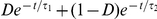 (
( values, PMG
0.91
values, PMG
0.91 0.98, MG5 0.81
 0.95), showing that
the free microglia cell motility involves both a strong short-range directional
correlation due to the existence of small ‘runs’ (with the time
constant
0.95), showing that
the free microglia cell motility involves both a strong short-range directional
correlation due to the existence of small ‘runs’ (with the time
constant  ) and a long-range directional persistence mediated by
the zigzag turning preference (with the time constant
) and a long-range directional persistence mediated by
the zigzag turning preference (with the time constant
 ).
).
Figure 2. Zigzag preference of crawling PMG and MG5 cells.

A) Typical return maps of turning angles  (red, PMG;
blue, MG5), B) Histograms of the zigzag preference
(red, PMG;
blue, MG5), B) Histograms of the zigzag preference
 (n = 8 for each case), C) Auto-correlation
functions of
(n = 8 for each case), C) Auto-correlation
functions of  and their
corresponding fits to an exponential function, D) and E)
Auto-correlation functions of the instantaneous direction of movement
for PMG and MG5 cells, respectively (n = 8 for each
case). F) Histograms of the two time constants obtained by fitting the
curves in (D) and (E) to
and their
corresponding fits to an exponential function, D) and E)
Auto-correlation functions of the instantaneous direction of movement
for PMG and MG5 cells, respectively (n = 8 for each
case). F) Histograms of the two time constants obtained by fitting the
curves in (D) and (E) to  .
.
 cos
cos in (D) and
(E) are the ensemble time average over the entire observation duration
of the inner-product between the two directional unit vectors separated
by
in (D) and
(E) are the ensemble time average over the entire observation duration
of the inner-product between the two directional unit vectors separated
by  .
.
Zigzag turns in a mathematical model cell
Few mathematical models have discussed the mechano-chemical aspects of cell
crawling, particularly for the long-term behavioral pattern of free cells.
Regarding the experimental observations on the crawling pattern of amoebae, Li
et al. proposed a simple mathematical model to describe the
dynamics of the instantaneous direction of motion
 [15]. The model
was basically a noise-driven damped linear oscillator that was facilitated by
low frequency white noise. Although the proposed model could produce some of the
essential features, such as the power spectral density function of
[15]. The model
was basically a noise-driven damped linear oscillator that was facilitated by
low frequency white noise. Although the proposed model could produce some of the
essential features, such as the power spectral density function of
 and the autocorrelation function of
 from their experimental data, it was a simple model
lacking a detailed connection to the biochemical reactions governing the cell
shape and crawling behavior. Recently, Nishimura et al.
[18] proposed a
more realistic model for cell locomotion and cytofission, and discussed the
important role of the actin polymerization-suppression factor, known as the
“cortical factor,” for determining the directional persistence of
cell migration. They found that the persistence could be changed significantly
by two parameters, the threshold value of actin polymerization and the rate of
transferring the cortical factor from the cytosol to the cortical layer.
from their experimental data, it was a simple model
lacking a detailed connection to the biochemical reactions governing the cell
shape and crawling behavior. Recently, Nishimura et al.
[18] proposed a
more realistic model for cell locomotion and cytofission, and discussed the
important role of the actin polymerization-suppression factor, known as the
“cortical factor,” for determining the directional persistence of
cell migration. They found that the persistence could be changed significantly
by two parameters, the threshold value of actin polymerization and the rate of
transferring the cortical factor from the cytosol to the cortical layer.
Another realistic mathematical model for crawling cell was developed recently by Satulovsky et al. [24]. It is a rule-based top-down model that incorporates some of the essential chemical and mechanical components of cell crawling. This general model was developed to understand how the signaling events controlling cell protrusion and retraction are coordinated to generate the shapes and migration patterns of different cell types. A range of migrating cells could be produced depending on the values of some key parameters, including Dictyostelium amoebae, fibroblasts, keratocytes, and neurons. In this study, the zigzag motility of this model cell was examined.
On a two dimensional surface, a simply closed loop, whose boundary can protrude
by a local activation signal or retreat in response to a global inhibition
signal, was modeled as a cell. The local activator
 induces the polymerization of actins, which moves the
cell boundary in the forward direction of movement. On the other hand, the
global inhibitor,
induces the polymerization of actins, which moves the
cell boundary in the forward direction of movement. On the other hand, the
global inhibitor,  , dissociates the
actin network and retreats the cell boundary toward the center of the cell if
, dissociates the
actin network and retreats the cell boundary toward the center of the cell if
 . Therefore, the moving front is activator rich, whereas
the tail part is inhibitor rich. The growth rate of
. Therefore, the moving front is activator rich, whereas
the tail part is inhibitor rich. The growth rate of
 is a nonlinear function of
 and
and  , and the
concentration of the inhibitor
, and the
concentration of the inhibitor 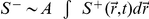 , where
 is the area enclosed by the model cell boundary. The
model also includes a stochastic process for the formation (and dissociation) of
focal adhesion sites: For every iterative time step, each point along the cell
boundary has some likelihood of adhesion to and detachment from the substrate
with a probability
is the area enclosed by the model cell boundary. The
model also includes a stochastic process for the formation (and dissociation) of
focal adhesion sites: For every iterative time step, each point along the cell
boundary has some likelihood of adhesion to and detachment from the substrate
with a probability  and
and
 , respectively.
Figure 3 shows four different
model cell trajectories obtained by changing one of the key parameters,
 , which is the decay rate constant of
 . The directional persistence of the model cell
trajectory varies significantly as a function of
. The directional persistence of the model cell
trajectory varies significantly as a function of  (see Fig. 4A). For example, for
 the linear regime ends below
 , whereas for
  it extends over
 . The visual similarity of the model cell (Fig. 4B) to the real microglia
(Fig. 1A) is quite
striking. Moreover, the trajectories of the model cell can also be viewed as a
sequence of small ‘runs’ and ‘turns’ as shown in Fig. 4B. The probability
distribution of turning angles
. The visual similarity of the model cell (Fig. 4B) to the real microglia
(Fig. 1A) is quite
striking. Moreover, the trajectories of the model cell can also be viewed as a
sequence of small ‘runs’ and ‘turns’ as shown in Fig. 4B. The probability
distribution of turning angles  , inter-turn
distances
, inter-turn
distances  , inter-turn time intervals
 , and inter-turn average velocities
 (see Fig. S4) are similar to those obtained in the
experiments with PMG and MG5 cells (see Fig. S2). Occasionally, the model cell also
shows front-splitting events as shown in Fig. S3 similar to the case of the PMG cell.
In addition, the model cell trajectories also favor zigzag turns, which are
again well captured in the return map of
(see Fig. S4) are similar to those obtained in the
experiments with PMG and MG5 cells (see Fig. S2). Occasionally, the model cell also
shows front-splitting events as shown in Fig. S3 similar to the case of the PMG cell.
In addition, the model cell trajectories also favor zigzag turns, which are
again well captured in the return map of  (see Fig. 4C). Moreover, the
auto-correlation function of
(see Fig. 4C). Moreover, the
auto-correlation function of  (Fig. 4D) shows that the memory
of the last turn affects only the current turn and decays quickly thereafter. As
in the case of microglia crawling trajectories, the function
(Fig. 4D) shows that the memory
of the last turn affects only the current turn and decays quickly thereafter. As
in the case of microglia crawling trajectories, the function
 cos
cos , measuring the
directional persistence, of the model cell was well fitted to a sum of two
exponential functions (Fig.
4E). Again,
, measuring the
directional persistence, of the model cell was well fitted to a sum of two
exponential functions (Fig.
4E). Again,  and
and
 correspond to the two time scales, one for the small
‘runs’ and the other for the long-range directional persistence. The
measured value of
correspond to the two time scales, one for the small
‘runs’ and the other for the long-range directional persistence. The
measured value of  changes
significantly (
changes
significantly ( 10 fold) as
 changes from 0.01 to 0.20 with its maximum value near
 as shown in Fig. 4F.
Figure 3. Centroid trajectories of the crawling model cells for different
parameter values of  .
.

The other parameter values were fixed as follows:

 m/s,
m/s,  1/s,
1/s,

 /s,
/s,  ,
,
 1/(s
1/(s
 m),
m),
 1/
1/ m,
m,
 1/s,
1/s,
 1/
1/ m
m ,
,
 ,
,
 ,
,

 m. Each frame is
1000
m. Each frame is
1000 1000
1000
 m
m and
includes 200000 iteration steps.
and
includes 200000 iteration steps.
Figure 4. Long-range directional persistence and zigzag turns of the crawling trajectories of a mathematical model cell.

A) Mean square displacements vs. time for  (red),
 (blue),
 (violet),
and
(violet),
and  (green). The cyan and black dotted lines have a
slope of 1 and 2, respectively. B) Close-up view of the green
highlighted segment in Fig.
3 (
(green). The cyan and black dotted lines have a
slope of 1 and 2, respectively. B) Close-up view of the green
highlighted segment in Fig.
3 ( ). Some
snapshot images of the crawling cell are superimposed on the trajectory.
The red (blue) boundary is the moving front (trailing edge) where
). Some
snapshot images of the crawling cell are superimposed on the trajectory.
The red (blue) boundary is the moving front (trailing edge) where
 (
( ). The
inset plots the instantaneous local curvature along the centroid
trajectory. Local maxima and minima are marked by red dots, which
correspond to the turning points (black dots) along the centroid
trajectory. C) Return map of the turning angle
(
). The
inset plots the instantaneous local curvature along the centroid
trajectory. Local maxima and minima are marked by red dots, which
correspond to the turning points (black dots) along the centroid
trajectory. C) Return map of the turning angle
( ). The
zigzag preference
). The
zigzag preference  . D)
Auto-correlation function of the sequence of turning angles
(
. D)
Auto-correlation function of the sequence of turning angles
( ). The blue
dotted line is an exponential function fit with a decay time constant of
0.705. E) Auto-correlation functions of the instantaneous direction of
movement for
). The blue
dotted line is an exponential function fit with a decay time constant of
0.705. E) Auto-correlation functions of the instantaneous direction of
movement for  (red),
 (blue),
 (violet),
and
(violet),
and  (green). F) Two time constants obtained by
fitting
(green). F) Two time constants obtained by
fitting  cos
cos to
to
 . The error
bars represent the standard deviation based on 10 different trajectories
obtained with a different initial condition.
. The error
bars represent the standard deviation based on 10 different trajectories
obtained with a different initial condition.
Changing  affects a number of different features of the cell
trajectory simultaneously as shown in Fig. 5. As
affects a number of different features of the cell
trajectory simultaneously as shown in Fig. 5. As  changes from 0.01
to 0.20,
changes from 0.01
to 0.20,  ,
,  ,
,
 , and
, and  , change by
26.6%, 96.3%, 128.8%, and 76.6%, in that order, with
respect to their corresponding minimum values. The minimum of
, change by
26.6%, 96.3%, 128.8%, and 76.6%, in that order, with
respect to their corresponding minimum values. The minimum of
 , the maxima of
  ,
,
 and
and  all are closely
located around
all are closely
located around  . Of course, the
smaller
. Of course, the
smaller  is or the larger
  ,
,
 and
and  are, the larger
 becomes. Therefore, in the simulations
 ,
,  ,
,
 and
and  all contribute
synergetically to the maximum peak of
all contribute
synergetically to the maximum peak of  near
near
 .
.
Figure 5. Various properties of the model cell trajectories:

A) mean zigzag preference factor, B) mean turning angle, C) mean inter-turn time interval, and D) mean inter-turn distance. The error bars indicates the s.d. for 10 different trials with a different initial condition.
Discussion
The moving trajectories of the freely crawling rat microglia and mouse-derived
microglia cell line, which had been grown in culture for 2–4 days, were
analyzed carefully by long-term time-lapse video imaging. The trajectories could be
viewed as a chain of small ‘runs,’ and in many cases two successive
angles connecting the runs along the chain were not random but anti-correlated. This
anti-correlation is statistically significant. In addition, similar behavior was
identified in a simple rule-based model cell that incorporates the biochemistry of
actin polymerization/depolymerization of the cell shape regulation. The properties
of the model cell trajectories, as characterized by  ,
,
 ,
,  ,
,
 ,
,  ,
,
 and
and  , could be changed
significantly by varying the decay rate
, could be changed
significantly by varying the decay rate  of the activator
species associated with actin polymerization. These findings are consistent with
those reported by Li et al.
[15] regarding the
motility of starving Dictyostelium amoebae. Table 1 lists various quantities of dicty cells
as well as PMG, MG5, and the model cell.
of the activator
species associated with actin polymerization. These findings are consistent with
those reported by Li et al.
[15] regarding the
motility of starving Dictyostelium amoebae. Table 1 lists various quantities of dicty cells
as well as PMG, MG5, and the model cell.
Soon after Li's work on dicty cell motility, Maeda et al.
[16] published an
interesting article on a closely related issue. They examined the dynamics and
statistics associated with the cell shapes of crawling dicty cells in their moving
frames. They identified three distinct dynamical states, elongated, rotating, and
oscillating, and found that it was typical of crawling dicty cells to have abrupt
transitions among these different states. No detailed statistics regarding the time
intervals associated with the transitions were provided. The period of oscillation
for the oscillatory states was typically  min, which is similar
to what Li et al. reported for the mean inter-turn time interval
(
min, which is similar
to what Li et al. reported for the mean inter-turn time interval
( min). The oscillatory state can be viewed as an unusual case
in which all successive turns result in a quite regular zigzag pattern, even though
Li's work reported that the dicty memory is only short-range rarely extending
over one turn. This contradiction can originate from the difference in the
characteristics of the cells being investigated or in the environments to which the
cells were subjected to.
min). The oscillatory state can be viewed as an unusual case
in which all successive turns result in a quite regular zigzag pattern, even though
Li's work reported that the dicty memory is only short-range rarely extending
over one turn. This contradiction can originate from the difference in the
characteristics of the cells being investigated or in the environments to which the
cells were subjected to.
Regarding the regular oscillatory behavior of crawling cells, Barnhart et al. [1] reported a robust “bipedal locomotion” of crawling fish epithelial keratocytes. They found persistent oscillatory movement in which retraction of the trailing edge on one side of the cell body is out of phase with retraction of the other side. In other words, the trailing edge oscillation is the key for keratocyte locomotion, whereas the front dynamics is believed to be the key component in the navigation of crawling amoebae and microglia. The authors also provided a mathematical model viewing the keratocytes as a three-component stick/slip elastic system, in which a leading front is coupled mechanically to the left and right portion of the tailing edge. Nonlinear elastic coupling between the front and tail was the key for rendering the lateral periodic oscillation of the cell body. One important result of their model is the positive correlation between the mean cell speed and oscillation frequency. As an analogy, PMG and MG5 cells also show a positive correlation between the average cell speed and the inverse of the average inter-turn time interval (not shown).
Directional persistence of crawling cells was also discussed in several other recent reports. For example, Selmeczi et al. [25] investigated the motile patterns of human keratincocytes and fibroblasts, and found that some key properties of much studied OU model conflicted with their experimental data. With an extra term, which carries the memory of past velocities, added to the simple OU model, however, they could better describe the trajectories of the cells. Another study on the crawling behavior of freely moving cells was reported recently by Dieterich et al. [6]. They observed anomalous cell migrations of renal epithelial Madin-Darby kidney cells and reported that their crawling paths were best described by the fractional Klein-Kramers equation which involved temporal memory. Once again, it was indicated that neither the worm-like chain model nor the simple OU model were suitable for describing the crawling cells of their concern. The mathematical models proposed by Selmeczi et al. or Dieterich et al. may also be applicable to dicty amoebae and microglia, since both models have components for data-driven tailoring of cell-specific type. These two reports, however, do not specifically discuss the zigzag turning behavior of crawling. But, we indicate that the moving trajectory of the epithelial cell reported in [6] could also be viewed as a sequence of ‘run-and-turns’ showing a strong tendency of zigzag turns.
In summary, the trajectories followed by freely crawling cells are viewed as a chain of ‘run-and-turns, ’ and then the cells appear to favor making zigzag turns. This contrasts with the well-known bacterial tumbling that results in the random selection of a moving direction. The cultured microglia of rat brains and MG5 cell lines as well as Dictyostelium amoebae are good examples of this zigzag motility hypothesis. Satulovsky's simple mathematical model cell incorporating only the essential biochemistry of actin polymerization and cell mechanics also generates a similar motile behavior. Taken all together, the observed zigzag turning behavior is believed to be a generic feature of many different crawling cells in isolation. The key biophysics that underlies the observed inherent zigzag motility might be due to the extension pattern of pseudopodia [4] and the spatiotemporal dynamics of the coherent actin waves [29]. However, the generality of the observed motile behavior and the underlying mechanisms need to be further tested using many other types of cells and models. Finally, we should indicate that the run-and-turn chain scenario is an interpretation that is forced on smooth trajectories of crawling cells: the trajectories themselves are not piecewise linear but differentiable. The main finding of this investigation is that crawling cells seem to prefer to have zigzag motility with a short-term memory, and our analyis leading to this conclusion does not require that the cell trajectories to be a piecewise linear chain.
Materials and Methods
Ethics Statement
All experimental procedures and protocols were in accordance with the guidelines established by the Committee of Animal Research Policy of Korea University College of Medicine.
Microglia cell culture
Primary glia co-cultures were prepared from the cerebral cortex of postnatal day
1–2 Sprague Dawley rat brains (Charles River, OrientBio Inc.). The brains
were excised quickly and the cerebral cortices were removed and cleared of
meninges under a dissecting microscope. After a papain (6 unit) treatment (10
min), fragmented cortical tissues were collected and dissociated mechanically
using a fire-polished Pasteur pipette in 2 ml of DMEM supplemented with
10% FBS. The dissociated cells were grown in T-75 culture flasks (BD
Falcon) (37 , 5% CO
 ) with an initial
seeding density of
) with an initial
seeding density of  cells/flask in 10
ml DMEM with 10% FBS. The culture medium was changed in every 5 days.
cells/flask in 10
ml DMEM with 10% FBS. The culture medium was changed in every 5 days.
After growth in T-75 flasks for several days, the cells were shaken with new
culture media at 120 rpm for 10 min to remove the dead cells, and subsequently
shaken at 280 rpm for 20 min to harvest the microglia cells detached from the
substrate. The supernatant was collected, centrifuged for 5 min at 1500 rpm, and
the microglia cells thus acquired were plated on a cover-slips (50
cells/mm ) for observation.
After plating, the cells were stabilized in an incubator
(37
) for observation.
After plating, the cells were stabilized in an incubator
(37 , 5% CO
 ) for three hours,
and the culture media was gently replaced with DMEM with 10% FBS to
further remove the dead cells. The same culture medium and protocol used for the
PMG cells after dissociation was used for MG5 cell culture. The MG5 cell line
was a gift from Dr. Ikeda at Toyama University, Japan.
) for three hours,
and the culture media was gently replaced with DMEM with 10% FBS to
further remove the dead cells. The same culture medium and protocol used for the
PMG cells after dissociation was used for MG5 cell culture. The MG5 cell line
was a gift from Dr. Ikeda at Toyama University, Japan.
Time-lapse imaging and data processing
Culture dishes containing the PMG (or MG5) plated cover-slips were placed in a
temperature  ) and CO
 (5%)
regulated home-built chamber mounted onto the stage of an inverted microscope
(IX71, Olympus) with an objective lens (20x, NA 0.55). Time-lapse images were
acquired at 15 sec intervals, typically for a time period longer than 24 hours,
using a cooled CCD camera (MFcool, ProGres) with a spatial resolution of 0.5
(5%)
regulated home-built chamber mounted onto the stage of an inverted microscope
(IX71, Olympus) with an objective lens (20x, NA 0.55). Time-lapse images were
acquired at 15 sec intervals, typically for a time period longer than 24 hours,
using a cooled CCD camera (MFcool, ProGres) with a spatial resolution of 0.5
 m/pixel. To trace out the trajectory of a crawling cell
and identify its turning events, the acquired images were binarized using the
ImageJ program and the centroid of the cell body was calculated for each frame.
We have assumed that the mass density is uniform. The sequence of the centroid
positions (X
m/pixel. To trace out the trajectory of a crawling cell
and identify its turning events, the acquired images were binarized using the
ImageJ program and the centroid of the cell body was calculated for each frame.
We have assumed that the mass density is uniform. The sequence of the centroid
positions (X ,Y
,Y ) [green dots
in Fig.
S5A] was low-pass filtered by locally fitting them separately to
a third order polynomial function with a sliding window of 11 successive points
[red solid lines in Fig. S5B and S5C], which corresponds to
150 sec in time or
) [green dots
in Fig.
S5A] was low-pass filtered by locally fitting them separately to
a third order polynomial function with a sliding window of 11 successive points
[red solid lines in Fig. S5B and S5C], which corresponds to
150 sec in time or  7
7
 m in space. The local curvature
 was calculated at each time step using the fitted
functions [blue dots in Fig. S5D]. Finally, a lowpass filter was
applied to
was calculated at each time step using the fitted
functions [blue dots in Fig. S5D]. Finally, a lowpass filter was
applied to  with a cutoff at 30 sec, and the local extrema of the
filtered
with a cutoff at 30 sec, and the local extrema of the
filtered  [black dots in Fig. 5D] were considered to be a turning
point.
[black dots in Fig. 5D] were considered to be a turning
point.
Fitting and filtering effects on the zigzag preference
Whether it is an experimental data or a simulation result, the centroid
trajectories of crawling cells have some high-frequency fluctuation due to
intrinsic physiological noise as well as errors in the imaging and data
processing. Then, the questions are how much do we smooth the raw data before we
identify a turning event as an extremum of the local curvature
 . As discussed in the previous section, the smoothing
process involves 1) a local fitting of the centroid positions to a third order
polynomial function and 2) a lowpass filtering of
. As discussed in the previous section, the smoothing
process involves 1) a local fitting of the centroid positions to a third order
polynomial function and 2) a lowpass filtering of
 . Naturally, the zigzag preference
 depends on the cutoff values that we introduced during
the smoothing process.
depends on the cutoff values that we introduced during
the smoothing process.
The size of the fitting window significantly influences the number of turning
events as shown in Fig. S6 and S7A: with
the smaller window size, the larger the number of turns becomes. The temporal
range (40 160 sec) that we have explored in Fig. S7A
corresponds to the spatial range of 4.2
160 sec) that we have explored in Fig. S7A
corresponds to the spatial range of 4.2 16.8
16.8
 m approximately, considering that the mean crawling
velocity is about 6.3
m approximately, considering that the mean crawling
velocity is about 6.3  m/min for the given
set of parameter values. This is a physical range in which the zigzag phenomenon
is relevant since the size (diameter) of the model cell is about
m/min for the given
set of parameter values. This is a physical range in which the zigzag phenomenon
is relevant since the size (diameter) of the model cell is about

 m. In other words, we are only interested in the zigzag
turns arising more or less at the physical size of a single cell. Since the
local fitting process has a spatial lowpass filtering effect, a window size that
is too small will results in too many uncorrelated noisy turns as shown in Fig. S7B.
On the contrary, a window size that is too big will wipe out the zigzag
information. Figure S7C plots the effect of the fitting window size on the zigzag
preference: it varies significantly but the zigzag turning preference remains
over the whole range being explored. After the local curvature
m. In other words, we are only interested in the zigzag
turns arising more or less at the physical size of a single cell. Since the
local fitting process has a spatial lowpass filtering effect, a window size that
is too small will results in too many uncorrelated noisy turns as shown in Fig. S7B.
On the contrary, a window size that is too big will wipe out the zigzag
information. Figure S7C plots the effect of the fitting window size on the zigzag
preference: it varies significantly but the zigzag turning preference remains
over the whole range being explored. After the local curvature
 was computed with the smoothed cell trajectories, a
(boxcar) lowpass filter was applied to
was computed with the smoothed cell trajectories, a
(boxcar) lowpass filter was applied to  to exclude very
small-angle high-frequency turns. The effect of the filter size on the total
number of turns and the zigzag preference is plotted in Fig. S8.
Again, they vary but the zigzag phenomenon remains the same. Our analysis on the
model cell trajectories given in Fig. 4 and Fig. S4 are based on the fitting window size
of 101 sec and the lowpass filter size of 21 seconds.
to exclude very
small-angle high-frequency turns. The effect of the filter size on the total
number of turns and the zigzag preference is plotted in Fig. S8.
Again, they vary but the zigzag phenomenon remains the same. Our analysis on the
model cell trajectories given in Fig. 4 and Fig. S4 are based on the fitting window size
of 101 sec and the lowpass filter size of 21 seconds.
Mathematical crawling cell model
The mathematical model cell proposed by Satulovsky et al.
[24] was
simulated to determine if it could exhibit the zigzag motile behavior observed
in the current experiments. A crawling cell was modeled as a simply closed
contour on a two-dimensional space, which evolves in space and time. The points
along the cell perimeter are represented as vectors
 with the centroid of the cell being the origin. The
concentration of the activator
with the centroid of the cell being the origin. The
concentration of the activator  is a local
variable, whereas the concentration of the inhibitor
is a local
variable, whereas the concentration of the inhibitor
 is a global variable. At each iteration time step, each
point along the perimeter can either advance, retreat, or does not move based on
the following set of rules. Retraction occurs when
is a global variable. At each iteration time step, each
point along the perimeter can either advance, retreat, or does not move based on
the following set of rules. Retraction occurs when
 , and the rate of retraction is governed by the following
stochastic equation:
, and the rate of retraction is governed by the following
stochastic equation:
| (1) |
where  is the constant
minimum radius and
is the constant
minimum radius and  is the retraction
rate constant. The function
is the retraction
rate constant. The function  selects the larger
value of
selects the larger
value of  and
and  . Protrusion occurs
when
. Protrusion occurs
when  at a rate governed by the following
equation:
at a rate governed by the following
equation:
| (2) |
where  is the average
protrusion rate and
is the average
protrusion rate and  is a random number
generated from a Gaussian distribution of the mean
is a random number
generated from a Gaussian distribution of the mean
 and variance
  . The evolution of
activator
. The evolution of
activator  is governed by the equation
| (3) |
The
first two terms are deterministic, whereas the third term is a stochastic
positive feedback loop accounting for both the local stimulation and the
existence of a random signal. The function  for
for
 and
and  for
for
 , where
  is a threshold
value for the feedback.
is a threshold
value for the feedback.  accounts for the
rate of random bursts cased by internal baseline activities. The function
accounts for the
rate of random bursts cased by internal baseline activities. The function
 again represents a random number generated from a
Gaussian distribution. The retraction signal is governed by a global inhibition
rule
again represents a random number generated from a
Gaussian distribution. The retraction signal is governed by a global inhibition
rule  , where
  is the inhibition
constant,
is the inhibition
constant,  is the total area of the cell, and the integration is a
line integral over the entire cell border, which is composed of 360 pixels
(i.e., 1 pixel for 1 degree with respect to the centroid). Each pixel
corresponds to 0.286
is the total area of the cell, and the integration is a
line integral over the entire cell border, which is composed of 360 pixels
(i.e., 1 pixel for 1 degree with respect to the centroid). Each pixel
corresponds to 0.286  m and one iteration
time step is one second. At each iterative time step, the formation of focal
adhesions and their detachments are assigned stochastically to the points along
the cell perimeter with a probability
m and one iteration
time step is one second. At each iterative time step, the formation of focal
adhesions and their detachments are assigned stochastically to the points along
the cell perimeter with a probability  and
and
 , respectively. Retraction is inhibited when a perimeter
point hits a focal adhesion. The biophysical justifications for the above set of
equations and the numerical iteration scheme are described in detail in
reference [24].
The values of the eleven parameters
, respectively. Retraction is inhibited when a perimeter
point hits a focal adhesion. The biophysical justifications for the above set of
equations and the numerical iteration scheme are described in detail in
reference [24].
The values of the eleven parameters  ,
,
 ,
,  ,
,
 ,
,  ,
,
 ,
,  ,
,
 ,
,  ,
,
 ,
,  used for the
numerical simulations are specified in the figure caption of Fig. 3.
used for the
numerical simulations are specified in the figure caption of Fig. 3.
Supporting Information
Mean velocity distribution of a PMG cell for different values of
 .
.
(TIF)
Probability density functions associated with the trajectories of PMG (red)
and MG5 (blue) cells: A) turning angle, B) inter-turn distance, C)
inter-turn time interval, and D) inter-turn mean velocity (error bar: SEM,
n = 8 for each case). The two straight lines in (C) are
an exponential function fit for  min: PMG
(slope = −2.9), MG5
(slope = −3.5).
min: PMG
(slope = −2.9), MG5
(slope = −3.5).
(TIF)
Sequence of snapshot images showing a ‘front-splitting’ event: A)
PMG cell and B) the model cell ( ). Each frame
is
). Each frame
is 
 for (A) and
 m
m for (B). The
green lines in (B) represent the path of the centroid.
for (B). The
green lines in (B) represent the path of the centroid.
(TIF)
Probability density functions associated with the trajectories of the model
cell: A) turning angle, B) inter-turn distance, C) inter-turn time interval,
and D) inter-turn mean velocity [ = 0.01 (red), 0.03 (blue), 0.10
(violet), and 0.20 (green)]. The straight line in (C) is an exponential
function fit for
= 0.01 (red), 0.03 (blue), 0.10
(violet), and 0.20 (green)]. The straight line in (C) is an exponential
function fit for  = 0.03 for
 min (slope = −1.26).
(TIF)
Defining turning points: A) a PMG cell trajectory (raw data: green, smoothed
data: red) with turning points marked by red dots, B) x-coordinates in time,
C) y-coordinates, and D) local curvature  computed with
the fitted values of
computed with
the fitted values of  and
and
 shown in (B) and (C). In (D), turning points are
marked by black dots. This trajectory data matches the supplementary Movie
S1.
shown in (B) and (C). In (D), turning points are
marked by black dots. This trajectory data matches the supplementary Movie
S1.
(TIF)
Fitting window size effect on the number of turns: (green) raw trace of model
cell trajectory for  , (black and
red dots) turning points obtained with a fitting window size of 101 sec and
51, respectively. Inset: blown-up image of the boxed area. The black line
within the inset is the smoothed trajectory obtained with the fitting window
size of 101. The result is based on 200000 seconds of iteration.
, (black and
red dots) turning points obtained with a fitting window size of 101 sec and
51, respectively. Inset: blown-up image of the boxed area. The black line
within the inset is the smoothed trajectory obtained with the fitting window
size of 101. The result is based on 200000 seconds of iteration.
(TIF)
Fitting window size effect on the zigzag preference factor
 : A) Number of turns vs. fitting window size, B)
Return maps of turning angle sequences, C)
: A) Number of turns vs. fitting window size, B)
Return maps of turning angle sequences, C)  vs. fitting
window size.
vs. fitting
window size.
(TIF)
Filter cutoff size effect on the number of turns (dots) and the zigzag preference (square).
(TIF)
A time-lapse movie showing a freely crawling rat microglia cell: (green line) smoothed centroid trajectory and (red dots) turning points.
(WMV)
Footnotes
Competing Interests: The authors have declared that no competing interests exist.
Funding: This work was supported by the Korean Ministry of Science and Technology (KOSEF grant: R17-2007-017-0100-0). The funders had no role in study design, data collection and analysis, decision to publish, or preparation of the manuscript.
References
- 1.Julicher F, Theriot JA, Barnhart EL, Allen GM. Bipedal locomotion in crawling cells. Biophys J. 2010;98:933–942. doi: 10.1016/j.bpj.2009.10.058. [DOI] [PMC free article] [PubMed] [Google Scholar]
- 2.Fulco UL, Lyra ML, Viswanathan GM, Bartumeus F, Catalan J. Optimizing the encounter rate in biological interactions: Levy versus brownian strategies. Phys Rev Lett. 2002;88:097901. doi: 10.1103/PhysRevLett.88.097901. [DOI] [PubMed] [Google Scholar]
- 3.Anderson RA, Berg HC. Bacteria swim by rotating their flagellar filaments. Nature. 1973;245:380–382. doi: 10.1038/245380a0. [DOI] [PubMed] [Google Scholar]
- 4.Haastert JMV, Bosgraaf L, Peter JM. The ordered extension of pseudopodia by amoeboid cells in the absence of external cues. PLoS ONE. 2008;4:e5253. doi: 10.1371/journal.pone.0005253. [DOI] [PMC free article] [PubMed] [Google Scholar]
- 5.Weijer CJ. Visualizing signals moving in cells. Science. 2003;300:96–100. doi: 10.1126/science.1082830. [DOI] [PubMed] [Google Scholar]
- 6.Preuss R, Schwab A, Dieterich P, Klages R. Anomalous dynamics of cell migration. Proc Natl Acad Sci USA. 2008;105:459–463. doi: 10.1073/pnas.0707603105. [DOI] [PMC free article] [PubMed] [Google Scholar]
- 7.Watkins NW, Freeman MP, Murphy EJ, Edwards AM, Phillips RA, et al. Revisiting levy flight search patterns of wandering albatrosses, bumblebees and deer. Nature. 2007;449:1044–1048. doi: 10.1038/nature06199. [DOI] [PubMed] [Google Scholar]
- 8.Chou W, Coates TD, Hartman RS, Lau K. The fundamental motor of the human neutrophil is not random: evidence for local non-markov movement in neutrophils. Biophys J. 1994;67:2535–2545. doi: 10.1016/S0006-3495(94)80743-X. [DOI] [PMC free article] [PubMed] [Google Scholar]
- 9.Ohsawa K, Imai Y, Nakamura Y, Honda S, Sasaki Y, et al. Extracellular atp or adp induce chemotaxis of cultured microglia through gi/o-coupled p2y receptors. Neurosci. 2001;21:1975–1982. doi: 10.1523/JNEUROSCI.21-06-01975.2001. [DOI] [PMC free article] [PubMed] [Google Scholar]
- 10.Dyer JRM, Pade NG, Musyl MK, Humphries NE, Queiroz N, et al. Environmental context explains levy and brownian movement patterns of marine predators. Nature. 2010;465:1066–1069. doi: 10.1038/nature09116. [DOI] [PubMed] [Google Scholar]
- 11.Bonner JT, editor. Princeton University Press, Princeton; 2008. The social amoebae: the biology of cellular slime molds. [Google Scholar]
- 12.Allen GM, Barnhart EL, Marriott G, Keren K, Pincus Z, et al. Mechanism of shape determination in motile cells. Nature. 2008;453:475–481. doi: 10.1038/nature06952. [DOI] [PMC free article] [PubMed] [Google Scholar]
- 13.Fetler L, Amigorena S. Brain under surveillance: the microglia patrol. Neuroscience. 2005;309:329–393. doi: 10.1126/science.1114852. [DOI] [PubMed] [Google Scholar]
- 14.Alonso-Latorre B, Rodriguez-Rodriguez J, Aliseda A, Del Alamo JC, Meili R, et al. Spatio-temporal analysis of eukraryotic cell motility by improved force cytometry. Proc Natl Acad Sci USA. 2007;104:13343–13348. doi: 10.1073/pnas.0705815104. [DOI] [PMC free article] [PubMed] [Google Scholar]
- 15.Cox EC, Li L, Norrelykke SF. Persistent cell motion in the absence of external signals: a search strategy for eukaryotic cells. PLoS ONE. 2008;3:e2093. doi: 10.1371/journal.pone.0002093. [DOI] [PMC free article] [PubMed] [Google Scholar]
- 16.Matsuo MY, Iwaya S, Sano M, Maeda YT, Inose J. Ordered patterns of cell shape and orientational correlation during spontaneous cell migration. PLoS ONE. 2008;3:e3734. doi: 10.1371/journal.pone.0003734. [DOI] [PMC free article] [PubMed] [Google Scholar]
- 17.Helmchen F, Nimmerjahn A, Kirchhoff F. Resting microglial cells are highly dynamic surveillants of brain parenchyma in vivo. Science. 2005;308:1314–1318. doi: 10.1126/science.1110647. [DOI] [PubMed] [Google Scholar]
- 18.Sasai M, Nishimura SI, Ueda M. Cortical factor feedback model for cellular locomotion and cytofission. PLoS Comp Biol. 2009;5:e1000310. doi: 10.1371/journal.pcbi.1000310. [DOI] [PMC free article] [PubMed] [Google Scholar]
- 19.Drescher K, Gollub JP, Goldstein RE, Polin M, Tuval I. Chlamydomonas swims with two “gears” in eukaryotic version of run-and-tumble locomotion. Science. 2009;325:487–490. doi: 10.1126/science.1172667. [DOI] [PubMed] [Google Scholar]
- 20.Mackay SA, Potel MJ. Pre-aggregative cell motion in dictyostelium. J Cell Sci. 1979;36:281–309. doi: 10.1242/jcs.36.1.281. [DOI] [PubMed] [Google Scholar]
- 21.Clark P, Ridley A, Peckham M, editors. United Kingdom: John Wiley & Sons; 2004. Cell Motility: From Molecules to Organisms. [Google Scholar]
- 22.Colby RH, Rubinstein M, editors. New York: Oxford University Press; 2003. Polymer physics. [Google Scholar]
- 23.Raposo EP, da Luz MGE, Santos MC, Viswanathan GM. Optimization of random searches on regular lattices. Phys Rev E. 2005;72:046143. doi: 10.1103/PhysRevE.72.046143. [DOI] [PubMed] [Google Scholar]
- 24.Lui R, Satulovsky J, Wang Y-I. Exploring the control circuit of cell migration by mathematical modeling. Biophys J. 2008;94:3671–3683. doi: 10.1529/biophysj.107.117002. [DOI] [PMC free article] [PubMed] [Google Scholar]
- 25.Hagedorn PH, Larsen NB, Flyvbjerg H, Selmeczi D, Mosler S. Cell motility as persistent random motion: theories from experiments. Biophys J. 2005;89:912–931. doi: 10.1529/biophysj.105.061150. [DOI] [PMC free article] [PubMed] [Google Scholar]
- 26.Stossel TP. On the crawling of animal cells. Science. 1993;260:1086–1094. doi: 10.1126/science.8493552. [DOI] [PubMed] [Google Scholar]
- 27.Ornstein LS, Uhlenbeck GE. The discrete unlenceck-ornstein process. Phys Rev. 1930;36:823–841. [Google Scholar]
- 28.Chen M, Ouyang K, Song S-L, Wei C, Wang X, et al. Calcium flickers steer cell migration. Nature. 2009;457:901–906. doi: 10.1038/nature07577. [DOI] [PMC free article] [PubMed] [Google Scholar]
- 29.Burroughs NJ, Whitelam S, Bretschneider T. Transformation from spots to waves in a model of actin pattern formation. Phys Rev Lett. 2009;102:192103. doi: 10.1103/PhysRevLett.102.198103. [DOI] [PubMed] [Google Scholar]
Associated Data
This section collects any data citations, data availability statements, or supplementary materials included in this article.
Supplementary Materials
Mean velocity distribution of a PMG cell for different values of
.
(TIF)
Probability density functions associated with the trajectories of PMG (red)
and MG5 (blue) cells: A) turning angle, B) inter-turn distance, C)
inter-turn time interval, and D) inter-turn mean velocity (error bar: SEM,
n = 8 for each case). The two straight lines in (C) are
an exponential function fit for min: PMG
(slope = −2.9), MG5
(slope = −3.5).
(TIF)
Sequence of snapshot images showing a ‘front-splitting’ event: A)
PMG cell and B) the model cell (). Each frame
is
for (A) and
m for (B). The
green lines in (B) represent the path of the centroid.
(TIF)
Probability density functions associated with the trajectories of the model
cell: A) turning angle, B) inter-turn distance, C) inter-turn time interval,
and D) inter-turn mean velocity [ = 0.01 (red), 0.03 (blue), 0.10
(violet), and 0.20 (green)]. The straight line in (C) is an exponential
function fit for = 0.03 for
min (slope = −1.26).
(TIF)
Defining turning points: A) a PMG cell trajectory (raw data: green, smoothed
data: red) with turning points marked by red dots, B) x-coordinates in time,
C) y-coordinates, and D) local curvature computed with
the fitted values of and
shown in (B) and (C). In (D), turning points are
marked by black dots. This trajectory data matches the supplementary Movie
S1.
(TIF)
Fitting window size effect on the number of turns: (green) raw trace of model
cell trajectory for , (black and
red dots) turning points obtained with a fitting window size of 101 sec and
51, respectively. Inset: blown-up image of the boxed area. The black line
within the inset is the smoothed trajectory obtained with the fitting window
size of 101. The result is based on 200000 seconds of iteration.
(TIF)
Fitting window size effect on the zigzag preference factor
: A) Number of turns vs. fitting window size, B)
Return maps of turning angle sequences, C) vs. fitting
window size.
(TIF)
Filter cutoff size effect on the number of turns (dots) and the zigzag preference (square).
(TIF)
A time-lapse movie showing a freely crawling rat microglia cell: (green line) smoothed centroid trajectory and (red dots) turning points.
(WMV)