Energetic Basis of Correlation Between Catch-Up Growth, Health Maintenance, and Aging

Abstract

Catch-up growth, referring to infants with low birth weight reaching or exceeding normal body weight later in life, is negatively correlated to adult health outcome and life span. Life history theories have suggested that there exist trade-offs between early development and later health maintenance, but detailed mechanisms and the currency of the trade-off are unclear. In this paper, we present a general theoretical model for quantitatively elucidating the trade-off between growth rate and health maintenance in mammals from an energetic viewpoint. Based on the fundamental principles of energy conservation and organisms’ energy budgets, our model analyzes the allocation of metabolic energy to growth and health maintenance in different sets of prenatal and postnatal environments. Our model also implies a relationship between growth rate and the general process of aging. Life-span predictions are supported by quantitative and qualitative empirical observations and offer theoretical frameworks for future experimental designs and data analyses.

IT has been known for more than two decades that mammalian birth weight is negatively correlated to adulthood health. Infants with low birth weight (LBW) are more likely to develop adult-onset hypertension, diabetes, cardiovascular disease, and other metabolic syndromes (1–4). These observations have led to the hypothesis of “fetal origin of adult disease.” This hypothesis suggests that poor embryonic and fetal environments lead to LBW, which can go on to induce structural and functional abnormalities that cause permanently altered function of key organs, such as the kidney, heart, and pancreas (1–6). However, some studies have shown that these abnormalities may not appear in LBW infants until later in life (eg, (7–9)). More importantly, although some studies show the direct association between LBW and adult health, a considerable amount of evidence shows that the negative influence of LBW on later health is not apparent unless postnatal growth rate is taken into account and postnatal weight is adjusted (see reviews in (2,10,11)). Attempting to combine the influence of LBW and postnatal growth, Hale and Barker (11–14) refined the “fetal origin hypothesis” to propose a “thrifty phenotype hypothesis.” This hypothesis suggests that when the prenatal nutritional environment is poor, adaptive responses will optimize the growth of important organs, such as the brain, to the detriment of other organs, leading to LBW. However, the adaptations will be detrimental when nutrition is enriched and growth rates increase in the postnatal environment. Lucas and colleagues (10) further postulated, “when size in early life is related to later health outcomes only after adjustment for current size, it is probably the change in size between these points (postnatal centile crossing) rather than fetal biology that is implicated.” This postulation, along with the “thrifty phenotype hypothesis,” has been well supported by empirical observations. Many animal and clinical studies have shown that the catch-up growth, referring to that which allows infants with LBW to reach or exceed normal body weight later in life, increases the risk factor for adult diseases and shortened life spans (15–23).

Many efforts have been made toward an understanding of the “dangerous catch-up growth”(11). Several empirical studies revealed possible molecular and cellular mechanisms of the detrimental effects of catch-up growth (8,17,24), such as telomere attrition, reduction of β-cell mass, impaired antioxidant activities, and so on. But these studies were unable to reveal why it is that LBW-induced fast growth in a rich postnatal environment can yield adverse consequences later in life. Life history theories and empirical data have suggested the existence of trade-offs between early growth and later health (25–27), but the currency and detailed mechanisms of the trade-offs remain unclear. Several regression models have been proposed for analyzing the correlation between later health outcomes and early development variables (10), but no theoretical framework exists to offer quantitative guidelines as to how later health outcomes should be regressed on independent variables, such as birth weight, prenatal and postnatal growth rates, adult body mass, or others. In this paper, we present a general theoretical model for elucidating the trade-offs between catch-up growth and health maintenance in mammals. Based on the fundamental principles of energy conservation and organisms’ energy allocation strategies, our model analyzes the energetic efforts that an organism will make for growth and health maintenance in different sets of prenatal and postnatal environments and then makes quantitative and testable predictions on how growth rates, birth weights, adult body masses, and energy budgets affect that organism's health outcome, aging, and life span. Specifically, the model shows that if an individual with LBW has normal body mass later in life, then this individual must have experienced relatively faster postnatal growth. Because growth is energetically costly, this accelerated growth indicates that extra energy, which would otherwise be spent on somatic maintenance, will be channeled to growth, leading to higher levels of molecular or cellular damage. Thus, the individual with LBW and normal adult body mass will reach a certain mass-specific threshold of accumulated damage sooner, which will cause an earlier onset of certain diseases or of death.

METHODS

The definition of LBW varies and depends on the species and population under investigation. Many researchers have used the cutoff value of birth weight percentile, for example, the 10th percentile (10,28), whereas others have used the average birth weight of the population or species to discern an absolute value for normal weight below which LBW is defined (eg, see (2)). For example, in a study in Australia, the mean birth weight (SD) among 317 human infants was 2.712 ± 0.4 kg, and 35% had been defined as LBW (less than 2.5 kg) (29); the same value, 2.5 kg, was used in studies of populations in India and Finland (2,30). As far as we know, no studies have normalized birth weight data with respect to parents’ weights, although they are known to be correlated. Many studies have considered height and BMI as indices of body size (eg, see (2,28,30)), but in this model, we use body weight as the sole index. This method offers a departure point for more detailed models involving height. It should also be clarified that the coarse-grained model presented here only examines cases in which LBW is the sole abnormality, and LBW is usually caused by constrained fetal nutrient supply as investigated in many animal and clinical experiments (eg, see (26,31)). The LBW entangled with other birth diseases that are commonly attributed to non-nutritional factors, such as radiation, cigarette exposure, etc., are not discussed here.

Numerous aging theories exist, with some of the most popular being mutation accumulation (32), antagonistic pleiotropy (33), disposable soma (34), and recently, buffering mechanisms (35). Here, we focus and elaborate on the oxidative stress theory of aging, (eg, see (36,41), another leading theory amenable to theoretical approaches. This theory proposes that the dissipative mechanisms of oxidative metabolism and their subsequent deleterious productions (eg, reactive oxygen species [ROS]) cause various forms of molecular and cellular damage in nucleic acids, proteins, membranes, and mitochondria among others. Although organisms have efficient mechanisms to scavenge for ROS and repair or remove damaged molecules; some detrimental effects remain and accumulate and have become associated with the process of aging (36–41). Thus, we make the following simplifying assumptions:

(I) We assume that the rate of damage, H (in dimension of damaged mass/time), is proportional to the organism's metabolic rate (oxygen consumption rate), B, that is, H = ηB, where η is a constant in its dimension of mass/energy within a taxon. η is determined by two factors: the proportion of the dissipated metabolic energy that causes damage and the amount of biomass, such as polymeric linkage, that can be damaged by one unit of energy (see details in Appendix I). Here, with the first order of approximation, both H and η in this general model are collective quantities, which average over the damages in key organs and/or tissues contributing to aging and death. A more detailed model dealing with specific types of damage, such as DNA mutation or protein degradation in a specific key organ, will have specific values of H and η.

(II) We assume that the biological pathways for maintaining organisms’ integrities (eg, repairing damage and error checking) require metabolic energy and that the rate of maintenance, P (in units of repaired mass/time), is proportional to the rate of energy allocated to maintenance, B_maint, with a coefficient, ρ, which is a constant within a taxon (in dimension of mass/energy), that is, P = ρB_maint. Similar to η, ρ is the product of two factors: the proportion of B_maint that is spent on repair mechanisms and the amount of damaged biomass that can be repaired by one unit of energy.

(III) The oxidative stress theory of aging associates accumulated damage with the process of aging, allowing the assumption that the degree of aging can be measured by the fraction (percentage), F, of body mass that is damaged. When a critical value of F is reached, F = F_C, an organism will die. Again, F_C is assumed to be a constant within a taxon.

Here, we define a dimensionless constant, ϵ = ρ/η$\text{ϵ}=\text{ρ/η}$, as the ratio of repair coefficient to damage coefficient. This ratio is assumed to be a constant within a taxon. Under normal conditions in aging mammals, where accumulated damage increases (P < H), ϵ is less than 1, assuming B_maint = B in the adulthood (see later). However, under special conditions, as in the processes of rejuvenilization (P > H) and regeneration (P > H) or in the case of some ectotherms that seem not to age or to age very slowly (P ≈ H), ϵ ≥ 1, because B_maint ≤ B. It is difficult to calculate the exact value of ϵ from the first principles of physics and chemistry. However, an estimation based on some biological constants gives a lower bound of 0.99 (see Appendix I). Although there is no quantitative empirical data to test this prediction, there is limited qualitative experimental evidence that shows repair mechanisms having very high efficiency. First of all, there exist highly efficient scavenging systems in organisms to eliminate ROS generation, such as superoxide dismutase enzymes, peroxiredoxins, oxidized cyochorome c, and cytochrome oxidase, which efficiently lower the ROS damage (see review in (40,42). Second, there exist efficient repair/removal mechanisms for the macromolecular targets of ROS damage, including DNA, proteins, and lipids (eg, see review in (38,40,43)). For example, oxidized DNA bases are removed by base excision mechanisms, and DNA polymerase enzymes are able to identify and correct most types of errors. The oxidized methionine residues of proteins can be repaired by the enzyme methionine sulfoxide reductase, and oxidized proteins that cannot be repaired are removed by proteolysis either via lysosomal degradation or via the proteasome. In the case of membranes, three mechanisms are involved in efficient protection: lipid repair, lipid replacement, and scavenging of lipid peroxidation–derived end products.

Based on Assumptions I and II, the accumulated net damage at age T can be estimated as . Mathematically, the lower bound of the integral, t = 0, should start from conception. For mammals in early stages of pregnancy, particularly the embryonic period, oxygen concentrations in the embryo are particularly low, protecting the processes of blastulation and normal cell differentiation from oxidative stress (44,45). So, we assume that the damage rate, H, is negligible during the embryonic period (eg, for human, the first 7 weeks from fertilization), and the lower bound of the integral above, t = 0, starts at the beginning of the fetal period after the precursors of the major organs are formed. Relaxation of this assumption will not affect the conclusion of the model. Together, the fraction of the damaged body mass at time, T, is , where m(T) is the body mass at age T. This equation can be rewritten as

(1)

where, D(T) = F(T)/η, and again, ϵ = ρ/η is the ratio of repair coefficient to damage coefficient. D(T) can be considered the recalibrated mass-specific net damage and is in dimensions of energy/mass.

To carry out the calculation of equation (1), we need the detailed information of B and B_maint as functions of body mass and age over ontogeny. West and colleagues (46) proposed an ontogenetic growth model, which suggests that during growth, the whole-organism metabolic rate, B, is partitioned between the rate of energy allocated to synthesize new biomass, B_syn, and the rate of energy allocated to maintain existing biomass B_maint, that is, B = B_syn + B_maint. The first term can be expressed as B_syn = E_m dm/dt, where dm/dt is the growth rate and E_m is the amount of metabolic energy required to synthesize a unit of biomass. So the term, B_syn, corresponds to the “organizational work (or override) of growth” (47,48). The second term can be expressed as B_maint = B_mm, where the rate of energy allocated to maintenance, B_maint, is assumed to be linearly proportional to body mass because total cell number scales linearly with body mass, and on average, each cell requires approximately the same power for maintenance. Over ontogeny, the metabolic rate, B, scales with body mass, m, as B = B₀m^3/4, where B₀ is a normalization constant for a given taxon. This scaling relationship is predicted from allometric theories and supported by data on a diverse set of organisms, including mammals, birds, and fish (47,49,50). Then the growth equation can be written as

(2)

When growth stops, that is, dm/dt = 0, and an organism reaches its asymptotic mass, M, equation (2) gives B₀M^3/4 = B_mM and B_m = B₀M^−1/4.

The energy partition, equation (2), applies to both prenatal and postnatal growth (see (49,51) and Appendix II). Solving equation (2) with two different sets of parameters yields the curves of prenatal and postnatal growth, m_pre(t) and m_post(t):

(3a)

(3b)

where m_f is the initial mass of fetus; m₀ is the birth mass, which is the asymptotic mass in the prenatal curve, equation (3a), but the initial mass in postnatal curve equation (3b); M is the adult mass; and E_m,pre and E_m,post are the energies required to synthesize one unit of body mass prenatally and postnatally, respectively. These variables consider the energy for biosynthesis of tissue macromolecules from monomers, the cost of transport of molecules into and within cells, the cost of mechanical separation of nucleic acid strands and daughter cells during mitosis, etc. (48,52–54). E_m,pre and E_m,post are different in principle as they consider different growth environments. Empirical data also show that E_m,post is usually larger than E_m,pre for a given species ((51) and Appendix II).

Based on equation (2) when there is no growth, the rate of energy for maintenance, B_maint, equals B. So equation (1) becomes . But during growth, a considerable amount of energy is allocated to biosynthesis and B_maint = B − B_syn = B − E_m dm/dt. Substituting this relationship into equation (1) gives dm/m(T) at age, T, after birth, where T_f is the length of the fetal period. Because the mass ratios, m_f/m₀ and m₀/M, are very small, the integral in the first and third terms of this equation, which have the form of , can be calculated and simplified to be approximately, that is, m_pre(t) and m_post(t) can be treated as constants m₀ and M in the integrations (see details in Appendix III). Note: this equation can be integrated accurately, and similar conclusion can be drawn, but this approximation yields a simpler equation and clear biological meanings. The second and fourth terms of the equation are simply ϵE_m,pre (m₀ − m_f)/m(T) and ϵE_m,post (m(T) − m₀)/m(T). Together, we have the recalibrated mass-specific net damage at age T after birth, D(T)

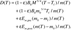(4)

Equation (4) is the major result of the model. In this equation, except for the repair coefficient to damage coefficients ratio, ϵ, all other parameters, namely, adult mass, M, birth mass, m₀, initial fetus mass, m_f, metabolic normalization constant, B₀, energy to synthesize one unit of biomass, E_m,pre and E_m,post, and length of fetal period, T_f, are not free parameters and can be independently measured for a given species. In the following section, we will show several predictions of equation (4) and suggest how to measure ϵ. The symbol, biological meaning, numerical values, and units of the parameters and variables in the model are listed in Table 1.

Table 1.

Symbols, Values, and Sources of the Parameters

Symbol	Biological Meaning	Value, Equation, and Dimension	Source
H	Rate of biomass damage	In mass/time	Assumption I
η	Coefficient in equation H = ηB	In mass/energy	Assumption I and Appendix I
P	Rate of biomass repairing	In mass/time	Assumption II
ρ	Coefficient in equation P = ρBmaint	In mass/energy	Assumption II
ϵ	Ratio of repair/damage coefficients,ϵ = ρ/η	Dimensionless; ϵ = 0.998	Appendix I and equation (8)
F	The fraction of biomass that are damaged	In percentage	Assumption III
D	The recalibrated mass-specific net damage	In energy/mass	Equation (1)
B	Metabolic rate	In energy/time	Equation (2)
Bmaint	Rate of energy allocation to maintain existing biomass	In energy/time	Equation (2)
Bsyn	Rate of energy allocated to synthesize new biomass	In energy/time	Equation (2)
B0	Normalization constant	0.0223 W/g0.75	(55)
Em,post	Energy required to synthesize one unit of biomass during postnatal growth	4,300 J/g	Appendix I, equation (3a), and Table 2
Em,pre	Energy required to synthesize one unit of biomass during prenatal growth	1,100 J/g	Appendix I, equation (3a), and Table 2
m0	Birth mass	In grams	Equation (3a)3b
M	Adult mass	In grams (600 g for rat)	Equation (3a)3b
mf	Initial mass of fetus	∼0.1 g (for rat)	Estimated from (56)
Tf	Length of fetal period	∼20 days (for rat)	Reference (56)
LS	Life span	In days	Equation (5)
C	Normalization of scaling relationship between gestation length and birth mass $T_{\text{f}}\sim C{m}_0^{1/4}$	C = −4 ln[1 − (mf/m0)1/4]	Reference (49) and Equation (7)
μ	Ratio of birth mass and adult mass	μ = m0/M	Equation (8)
r	Ratio of birth masses of catch-up growth and control animals	r = m0,1/m0,2	Equation (10)
R	Ratio of adult masses of catch-up growth and control animals	R = M1/M2	Equation (10)

RESULTS AND DISCUSSION

General Pattern of Aging and the Origin of Scaling Laws of Life Span

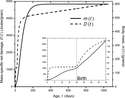
In Figure 1, we plot D(t) in equation (4) and the mass-specific net damage as a function of age, t. We have shown that during growth, D increases fast but that it slows down after the adult mass is reached, that is, m(t) = M, and D(t) becomes a linear function of t, the slope of which is (1 − ϵ) B₀M^−1/4.

Figure 1.

Growth curve (solid), m(t), and mass-specific net damage (dash), D(t), of a mammal whose adult mass is about 600 g. The inset is an expansion of the prenatal growth and damage curves and is calculated from equation (4) using prenatal growth variables and parameters. The values of the parameters in equation (4), which are used to produce the curves, are given in Table 1.

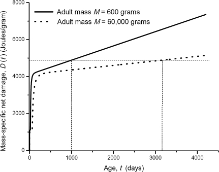
Using equation (4), we can compare the rate of aging and the life span of two organisms within a taxon with adult body masses M₁, and M₂, respectively. Equation (4) predicts that the mass-specific net damage, D(T), which reflects the degree of aging, will have a different slope for each organism, (1−ϵ)B₀M_1,2^−1/4. This is to say that the organism with larger adult mass ages more slowly as the slope of D(T) is smaller (Figure 2).

Figure 2.

The damage curves for animals whose adult masses are 600 and 60,000 g respectively. The horizontal dashed line is the hypothetic threshold of D(T) at which organisms die (Assumption III). The vertical dashed lines are the life spans of these two organisms.

According to Assumption III, when the life span of these two organisms, LS₁ and LS₂, is reached, they have the same mass-specific net damage, D₁(LS₁) = D₂(LS₂). For animals within a taxon, the values of ϵ, B₀, E_m, and the mass ratios, m_f/m₀ and m₀/M, are roughly the same, so this equation becomes

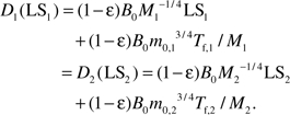Equation (3a) predicts that the length of fetal period, T_f, scales with the birth mass, m₀, to a ¼ power, that is, $T_{\text{f}}=C{E}_{m\text{,pre}}/B_0{m}_0^{1/4}$, where C = −4ln[1−(m_f / m₀)^1/4](49). This prediction is well supported by empirical data for 630 species of mammals (49). Because the mass ratio m₀/M is roughly the same within a taxon, we have $m_{\text{0,1}}{T}_{\text{f,1}}/M_1=m_{\text{0,2}}{T}_{\text{f,2}}/M_2$. Therefore the equation reduces to

(5)

Equation (5) predicts that the life spans of the organisms within a taxon will scale with the body mass to a ¼ power, that is, LS ∼ M^1/4. Empirical data on life span and body mass for mammals, birds, fish, and invertebrates strongly support this prediction (57–59).

Effects of the Catch-Up Growth on Aging and Life Span

In this section, we consider the case of catch-up growth in which two animals of the same species have the same initial fetus mass, m_f, but prenatal growth of Animal 1 is slower than that of Animal 2, so that they have different birth masses, m_0,1 < m_0,2. In contrast, postnatal growth is faster for Animal 1 than for Animal 2, so that after a certain age, τ, they have the same mass, m₁(T > τ) = m₂(T > τ) and, consequently, the same adult mass, M₁ = M₂. We are going to discuss the net mass-specific damage, D, of these two animals at the same age after birth, T − T_f. To simplify the discussion without losing generality, we consider the case in adulthood, that is, m₁(T − T_f) = m₂(T − T_f) = M. Similar conclusions can be drawn for the juvenile, that is, m₁(T − T_f) = m₂(T − T_f) < M.

According to equation (4), when m(T > τ) = M, the mass-specific net damage, D, becomes

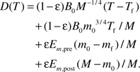(6)

First, we compare each term in equation (6) for Animal 1, D₁(T), and Animal 2, D₂(T), qualitatively.

• (1) Because M₁ = M₂, the first term of D₁ and D₂ are equal at the same ages after birth, T − T_f.

• (2) Because m_0,1 < m_0,2, the second term of D₁ is smaller than the one of D₂.

• (3) Because m_f is the same and m_0,1 < m_0,2, the third term of D₁ is smaller than the one of D₂.

• (4) Because M is the same and m_0,1 < m_0,2, the last term of D₁ is larger than the one of D₂.

The second and the third terms of D₁, which are associated with prenatal growth, are smaller than those of D₂. The first and the last terms of D₁, which are associated with postnatal growth, are either the same as or larger than the ones of D₂. This means that LBW and its subsequent catch-up growth generate more mass-specific damage during the postnatal growth (Term 4) in Animal 1, but this excess may be compromised by the difference in prenatal growth (Terms 2 and 3), so that the overall effect of LBW and catch-up growth on damage D may be zero.

Now, we compare D₁ and D₂ quantitatively. The difference between them can be calculated as

Recalling that the length of fetal period, T_f, scales with the birth mass, m₀, to a ¼ power, that is, $T_{\text{f}}=C{E}_{m\text{,pre}}/B_0{m}_0^{1/4}$, where C = −4ln[1−(m_f / m₀)^1/4] (49), we rewrite the equation above as

(7)

Equation (7) predicts that D₁ > D₂ if ϵ > C/(E_m,post/E_m,pre + C − 1). Data from 18 species of mammals with adult body mass ranging from 20 g to approximately 660 kg show that E_m,post is always larger than E_m,pre and the ratio of E_m,post/E_m,pre = 4.07 ± 3.17 (median = 2.84, N = 18; see Appendix II). This ratio means that it is energetically cheaper to synthesize one unit of prenatal biomass than postnatal biomass. This ratio also explains why, after the asymptotic mass is corrected, the prenatal growth rate is faster than the postnatal growth rate ((51) and Appendix II). Taking E_m,post/E_m,pre = 4, we have the condition for D₁ > D₂: The repair coefficient to damage coefficient ratio, ϵ, must satisfy ϵ > C/(C + 3). Taking the ratio of initial mass of fetus and birth mass, m_f / m₀ ≈ 0.1–0.5% (Table 1), C is approximately equal to 0.8, therefore, ϵ > 0.21. As we estimate in Appendix I, most mammals have efficient repair mechanisms and a high value of ϵ with a lower bound of approximately 0.99, so the condition, ϵ > 0.21, indicates that in most mammals, the catch-up growth causes more damage and a poorer health outcome, that is, D₁ > D₂. Although the ratio E_m,post/E_m,pre is shown to be >1 for all 18 mammalian species tested, the rare case may exist in which a given species will have the ratio E_m,post/E_m,pre equal to or smaller than 1. In this case, the condition for D₁ > D₂ becomes ϵ > 1, indicating that the mammalian species under normal conditions (ϵ < 1) would not show any detrimental effects of catch-up growth.

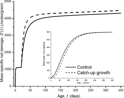
In Figure 3, we show the difference in D(t) that is due to catch-up growth. We consider two animals of the same species. The birth mass of Animal 1 (catch-up growth, dashed curves) is 15 g, whereas the one of Animal 2 (control, solid curves) is 45 g. Animal 1 grows slower than Animal 2 prenatally but faster postnatally (inset of Figure 3) so that they vary in birth mass but have the same adult mass (600 g, inset of Figure 3). As shown in Figure 3, after the adult mass is reached, that is, m(t > τ) = M, D(t) still increases with time. This is because ϵ is not 1, so the slope of D(t) in adulthood, (1 − ϵ) B₀M ^−1/4, is not zero. Figure 3 also shows that once the adult mass has been reached by both individuals, their rates of damage become the same; the same adult mass, M, gives the same slope of D(t), and the larger D in Animal 1 is due to the faster growth over ontogeny.

Figure 3.

The difference in mass-specific net damage, D(t), due to catch-up growth. The inset shows the growth curves of two animals of the same species. Both animals have the same adult mass (600 g). The birth mass of the catch-up growth animal (dashed line) is 15 g, and the one of the control animal (solid line) is 45 g. The curves are computed from equation (4); the values of other parameters are listed in Table 1. Note: The catch-up growth animal (Animal 1) has slower prenatal growth than the control animal (Animal 2), so the total net damage is smaller in Animal 1. In equation (6), we compare the mass-specific damage in adulthood, and the mass in the denominator is adult mass, M, which is the same for both individuals. So, the second and third terms in equation (6) of Animal 1, which represent the damages associated with prenatal growth, are smaller than those of Animal 2. However in this figure, D(t) during prenatal growth is calculated as the total net damage divided by the prenatal masses at time t, so the smaller total damage in Animal 1 is cancelled out by the smaller body mass of Animal 1. Therefore, the rate of mass-specific damage, D(t), during prenatal growth is almost the same in Animals 1 and 2 as shown in this figure.

Based on Assumption III, when two animals reach their life span, LS₁ and LS₂, the mass-specific net damage D₁(LS₁) = D₂(LS₂). Similarly, we can assume that a certain disease occurs at age t, when the damage has accumulated to a threshold, that is, D₁(t) = D₂(t) at the onset age of the disease, t. Based on this assumption, we can estimate the difference in life span or the onset age of a certain disease. Using equation (6) and $T_{\text{f}}=C{E}_{m\text{,pre}}/B_0{m}_0^{1/4}$, we derive

(8)

where μ = m₀/M is the ratio of birth mass and adult mass.

Equation (8) makes a quantitative and testable prediction of how differences in birth mass influence the life span (or the onset age of a certain disease) in the case of catch-up growth. It also predicts that within a taxon, where the repair coefficient to damage coefficient ratio, ϵ, and energy required to synthesize one unit of biomass, E_m, are roughly the same for the same difference in birth mass ratio (μ₂ − μ₁), the difference in life span scales with the adult mass, M, to a ¼ power, M^1/4. Due to the lack of empirical data on the differences in life span, birth mass, growth rate, and adult mass, we cannot test the predictions of equation (8) quantitatively. Nevertheless, its predictions are in qualitative agreement with the empirical observation.

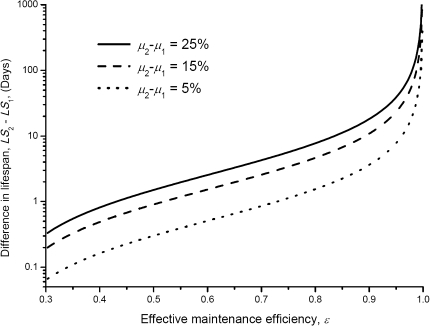
In Figure 4, we show how the life-span difference, LS₂ − LS₁, depends on the value of ϵ. When ϵ is close to 1, the life-span difference increases in the manner of ϵ/(1−ϵ). So, significant differences between the life spans of control and catch-up growth animals require high values of ϵ. Equation (8) offers a theoretical framework to the estimate value of ϵ. Here, we give an example: Let us assume that for two groups of rats with adult mass M = 600 g, the birth mass m₂ = 45 g and m₁ = 15 g, that is, μ₂ = 7.5% and μ₁ = 2.5%, and the life-span difference LS₂ − LS₁ is about 6 months, that is, 180 days. Taking C ∼ 0.8, E_m,post ∼ 4,300 J/g, E_m,pre ∼ 1,100 J/g, and B₀ = 0.0223 W/g^3/4, equation (8) gives ϵ ∼ 0.998 in agreement with the estimation of the lower bound of ϵ, 0.99, in Appendix I.

Figure 4.

Life-span difference versus birth mass ratio for four different adult masses. The curves are computed from equation (8). Parameter values for equation (8) are listed in Table 1.

Growth Rate and Life Span (or the onset age of diseases)

In this section, we discuss how life span or onset age of certain diseases is affected by growth rate. We consider several general cases in which the birth mass of Animal 1 is smaller than that of Animal 2, m_0,1 < m_0,2, but the growth of Animal 1 can be slower, equal to, or faster than Animal 2. Consequently, the ratio of adult masses, M₁/M₂, varies from smaller than 1 to larger than 1. According to Assumption III, animals from the same taxon have the same mass-specific damage, D, when their life spans have been reached or a certain disease presents, D₁(LS₁) = D₂(LS₂). To simplify the calculation without losing generality, we take the approximation of equation (6)

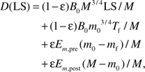where LS = T − T_f. We notice that $M^{3/4}/M>>m_0^{3/4}/M$ and LS >> T_f, so comparing to the first term, the second term is negligible; similarly, M − m₀ >> m₀ − m_f and E_m,post > E_m,pre, so comparing to the fourth term, the third term is negligible. Substituting the simplified equation (6) into D₁(LS₁) = D₂(LS₂), we have

(9)

We are going to discuss the predictions of equation (9) for different growth rates of Animal 1 and Animal 2.

Case 1: The growth rates of Animal 1 and Animal 2 are such that the mass ratios of these two animals are the same, that is, m_0,1/M₁ = m_0,2/M₂. In this case, equation (9) reduces to $M_1{\text{LS}}_1-M_2{\text{LS}}_2=0$. Because $M_1>M_2$, equation (9) predicts that LS₁ < LS₂.

Case 2: The growth rates of Animals 1 and 2 are such that M₁ < M₂, but there is still a small amount of catch-up growth so that M₁ is not too small and m_0,1/M1 < m_0,2/M₂. In this case, $M_1{\text{LS}}_1-M_2{\text{LS}}_2<0$ because$M_1^{-1/4}>M_2^{-1/4}$, equation (9) predicts that LS₁ < LS₂.

Case 3: The growth rates of Animals 1 and 2 are such that M₁ is much smaller than M₂ and m_0,1 /M₁ > m_0,2 /M₂. In this case, LS₁ can be larger, equal to, or smaller than LS₂ depending on the specific values of the parameters and variables in equation (9).

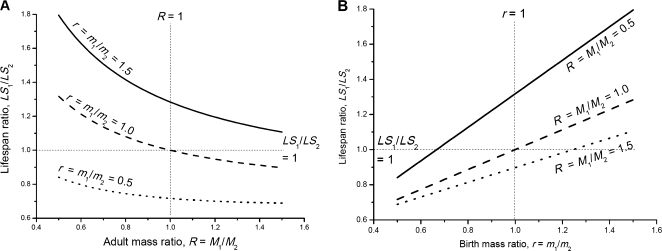
To compare the life spans of Animals 1 and 2 in these cases, we derive the ratio of life spans, LS₁/LS₂, from equation (9) and express it as a function of birth mass ratio, r = m_0,1/m_0,2, and adult mass ratio, R = M₁/M₂:

(10)

The life-span ratio from equation (10), LS₁/LS₂, depends on the ratio of repair coefficient to damage coefficients, ϵ, birth mass, m₂, adult mass, M₂, and life span, LS₂, of Animal 2, which can be considered the control animal. For a given species with a given adult mass and life span, equation (10) predicts how the life-span ratio, LS₁/LS₂, of experimental (Animal 1) and control (Animal 2) groups will change with differing mass ratios, R and r.

In Figure 5, we plot the life-span ratio as a function of adult mass ratio, R = M₁/M₂ (Figure 5A), and birth mass ratio, r = m_0,1/m_0,2 (Figure 5B), with a high value of ϵ, 0.998, which is estimated to cause a significant difference between the life spans of control and catch-up growth animals (equation (8) and Appendix I). From Figure 5A, we see the following: (a) when the birth mass ratio, r, is smaller than 1 (dotted curve, smaller birth mass of the experimental animal), the life-span ratio is also smaller than 1 for a broad range of adult mass ratio, R. In this case, larger R (larger M₁ and faster catch-up growth) leads to a smaller life-span ratio (short life span of Animal 1). Only when R is very small, that is, when M₁ is much smaller than M₂ (slower growth, instead of catch-up growth, of Animal 1), the life-span ratio, LS₁/LS₂, would be larger than 1; (b) when the birth mass ratio, r, is larger than 1 (solid curve, larger birth mass of the experimental animal), the life-span ratio is larger than 1 for a broad range of adult mass ratio, R. Only when R is very large (Animal 1 grows much faster than Animal 2) would the life-span ratio be smaller than 1. (c) When the birth mass ratio is equal to 1 (dashed curve), small R (R < 1, slower growth of animal 1) leads to large life-span ratio (LS₁/LS₂ > 1) and large R (R > 1, faster growth of animal 1) leads to small life-span ratio (LS₁/LS₂ < 1). Similar conclusions can be drawn from Figure 5B. Here, we use the life-span ratio as a measure of relative health status and maintenance efforts of Animals 1 and 2, so Figure 5 also reveals the trade-off between growth rate and maintenance.

Figure 5.

Life-span ratio of experimental and control animals. (A) Life-span ratio, LS₁/LS₂, as a function of adult mass ratio, R = M₁/M₂, for different birth mass ratios, r = m_0,1/m0,2. (B) Life-span ratio, LS₁/LS₂, as a function of birth mass ratio, r = m_0,1/m0,2, for different adult mass ratios, R = M₁/M₂. The curves are computed from equation (10). The life span and adult mass of the control animal, LS₂, m₂, and M₂, are taken to be 2 years, 45 g, and 600 g, respectively. Values of other parameters in equation (10) are listed in Table 1.

In summary, our model quantitatively predicts that (a) interspecifically, larger organisms age more slowly and that the life span of an organism is inversely proportional to its mass-specific metabolic rate; (b) within a species, an individual experiencing catch-up growth will have a poorer health outcome and shorter life span than an individual not experiencing catch-up growth; and (c) the difference between life spans (or the age of certain disease onset) in control and catch-up growth individuals will increase with the birth mass ratio, and this difference is nonlinearly dependent on the repair coefficient to damage coefficient ratio, birth mass, adult mass, and life span of the control animal. These predictions are quantitatively and qualitatively supported by empirical observations and offer a theoretical framework for future experimental designs and data analyses.

Our model proposes the detailed mechanism of the trade-off between growth and health maintenance from an energetic viewpoint and makes a significant contribution to life history theories of aging (eg, the disposable soma theory, (34,60)) by offering a quantitative framework with independently measurable variables. The proposed mechanism agrees with empirical observations, for many researchers have found that individuals with catch-up growth have poor somatic maintenance, such as lower protein expressions of antioxidant enzymes, insulin insensitivity, shortened telomeres, etc. (4,15,17,21,22,24,61). The model presented here also makes quantitative and testable predictions, which are helpful for the analysis of empirical data and the design of future experiments. The effects of LBW, catch-up growth, and later body mass on health outcome and life span are entangled in the empirical data. Researchers have noticed that the positive or negative correlation between one of these variables and health outcome can be obscured by a negative or positive correlation between another one of these variables and health outcome (10,24). Because of this, Lucas and colleagues (10) have suggested that we investigate “whether postnatal growth influences later health in its own right or whether it is simply a modifying factor” of LBW. The authors proposed several regression models, which regress the later health outcome or life span on different independent variables, including early body size, later body size, and interactions of the two. Our model gives the theoretical guidelines for these regression models. The results of our model confirm the hypothesis of Lucas and colleagues that the adult health status cannot be predicted by birth mass alone, it is influenced by the whole growth trajectory. A straightforward test of our model might begin with two cohorts of high and LBW individuals, each of which would be subdivided into two groups: one experiencing food restriction and the other being fed ad libitum. Although some studies have been done along this vein, there has yet to be one like this, which measures all the relevant variables over ontogeny at once: growth rate, body mass, metabolic rate, and life span (or age at onset of a certain disease). Certainly, experiments that compound these analyses will be of great interest to the field aging research. Finally, the results of our model also suggest that human nutritional programs might need to reconsider their strategies about catch-up growth. Individuals having what is deemed LBW should be particularly conscious of their diets, insofar as they ration their food intake and make no attempts to “bulk up.” Empirical testing of our model's predictions in human participants will provide further insight as to how we can optimize health.

FUNDING

This work was supported by grants from the Ellison Medical Foundation Senior Scholar Award AG-SS-2235 and NIH grants R01-AG028872 and P01-AG027734.

Appendix I. Estimation of the Lower Bound of the Repair Coefficient to Damage Coefficient Ratio, ϵ

The mass-specific accumulated damaged at age T is . When the life span, LS, is reached, it can be expressed approximately as F(LS) = η(B − ϵB_maint) × LS/M), where ϵ = ρ/η. Solving this equation for ϵ, we have . We now try to estimate ϵ based on the quantities in this equation. Because the energy allocated to maintenance, B_maint, is equal to (during adulthood) or smaller than (during ontogeny) total energy B, B_maint ≤ B. If we take B_maint = B in this equation, we will have an estimation of the lower bound of ϵ:

As we defined in Assumption I, η is determined by two factors: the proportion of the dissipated metabolic energy that causes damage and the amount of biomass, such as polymeric linkage, that can be damaged by one unit of energy. For the first factor, it is estimated that approximately 0.2%–2% of the oxygen consumed by cells is converted by mitochondria to ROS (42,43). So, we assume that ∼1% of the metabolic energy is associated with cellular or molecular damage. For the second factor, the energy associated with one unit of biomass damage is comparable to the energy required for one unit of biomass biosynthesis, such as the free energy to synthesize polymeric linkages from monomers. Theoretical consideration based on the first principles of biochemistry suggests that energy for biosynthesis ranges from 260 to 690 J/g (48,52,53,62) with an average ∼ 470 J/g (for wet mass). So, we assume that 1 g of biomass is damaged by about 470 J, giving 2.1 × 10⁻³ g/J. Together, η = 1% × 2.1 × 10⁻³ g/J. Substituting η into the lower bound of ϵ yields ϵ = 1 − F × M/(2.1 × 10⁻⁵ B × LS. Using the physiological data of mammals more specifically, humans, M = 70 kg, B = 100 W, and LS = 70 years, we have ϵ = 1− 0.015 × F, where F is the threshold for fraction of damage that causes death. So, even if F = 100%, which is biologically unrealistic, ϵ is still as high as 0.985. If F ranges from 1% to 20%, then ϵ is estimated to range from 0.99985 to 0.997. Note: this estimation is the lower bound of ϵ, so the actual value of ϵ may be even higher.

Appendix II: Equations and Parameters for Prenatal Growth

Based on empirical data from 36 species of bird and 18 species of mammal, Ricklefs (51) has recently shown that the embryo mass growth curve can by described by sigmoidal Gompertz functions. The Gompertz function has the following format:

(11)

where m₀ and m_f are defined as in equation (3a)3b, that is, m₀ is the asymptotic mass of the prenatal growth curve, and m_f is the initial mass of fetus; k is a growth rate constant (per time). We are going to show that equation (11) and equation (3a), $m_{\text{pre}}\left(t\right)={(1-[1-{(m_f/m_0)}^{1/4}\left]{\text{e}}^{-B_{0}t/4/E_{m\text{,pre}}/m_0}\right)}^4{m}_0$, which is also a sigmoidal function, are approximately equivalent, and consequently, the coefficients of the time-dependent term in these functions are the same, that is, $k=B_0/4/E_{m\text{,pre}}/m_0^{1/4}$.

We take the natural logarithm transform of both equations and then let μ = m_f/m₀ and $\text{α}=B_{0}t/4/E_{m\text{,pre}}/m_0^{1/4}$. This way, equation (11) becomes ln[m(t)] = ln[m₀] − ln[1/μ] × exp[−kt], and equation (3a) becomes ln[m(t)] = ln[m₀] + 4 ln[1−(1−μ^1/4) × exp[−at]]. Using the approximation ln(1 − x) ≈ − x, when x << 1, equation (3a) can be further transformed as ln[m(t)] = ln[m₀] − 4[1−μ^1/4] × exp[−at].

Now, we compare the two equations transformed from equation (11) and equation (3a): ln[m(t)] = ln[m₀] − ln[1/μ] × exp[−kt] and ln[m(t)] = ln[m₀] − 4[1−μ^1/4] × exp[−at]. Due to the approximation ln(1 − x) ≈ − x, the coefficient in equation (3a), 4(1 − μ^1/4), is slightly smaller than the coefficient in equation (11), ln[1/μ], when μ is much smaller than 1. But these two equations have the same exponential time dependence, that is, $k=B_0/4/E_{m\text{,pre}}/m_0^{1/4}$. This relationship is in good agreement with empirical data as Ricklefs (51) reported that embryo growth rate, k, decreases as the −¼ power of neonate size, m₀, that is, k ∼ m₀^−1/4. Similarly, it can be proved that the postnatal growth rate, k_post, can be expressed in terms of E_m,post and M (the adult mass) as k_post = B₀ / 4 / E_m,post/M^1/4

Ricklefs has estimated k_post and k for a broad range of mammals. From these values and the asymptotic values of pre- and postnatal Gompertz growth curves, m₀ and M, we can estimate the ratio of E_m,post and E_m,pre as E_m,post/E_m,pre = (m₀/M)^1/4 × (k_post/K). We also fit equations 3a and 3b with the empirical curves for postnatal growth (46,48) and prenatal growth (56) and estimated values of E_m,post and E_m,pre from these separated measured growth curves. In Table 2, we list the values of ratio E_m,post/E_m,pre from these estimations. The average value of the ratio is 4.07 ± 3.17 (median = 2.84, N = 18). This ratio means that it is energetically cheaper to synthesize one unit of prenatal biomass than one unit of postnatal biomass. Lower energetic costs of the fetus may be due to the facts that (a) the indirect cost of fetal growth, such as the cost of transporting nutrients and energy, is partially paid by the mother and (b) fetal cells and organs are less well differentiated and developed, therefore requiring less energy to grow.

Table 2.

Data Required to Estimate Ratio E_m,post/E_m,pre

Species	M (g)	kpost (per day)	m0 (g)	k (per day)	Em,post/Em,pre
Data from reference (51)
African antelope	37,800	0.0043	15,898.8	0.012	2.25
Cattle	661,000	0.0031	4,8050.1	0.012	2.01
Goat	59,700	0.0041	7,193.9	0.019	2.73
Guinea pig	982	0.0106	167.0	0.053	3.21
Elk	214,000	0.006	5,837.2	0.024	1.63
Human	61,300	0.0005	5,039.2	0.012	12.9
Snowshoe rabbit	1,570	0.0308	251.9	0.076	1.56
Rhesus monkey	7,990	0.0012	706.9	0.024	10.91
European rabbit	2,400	0.0228	817.3	0.073	2.45
Domestic sheep	70,500	0.0031	8,786.7	0.021	4.03
Olive baboon	8,060	0.0026	1,030.7	0.022	5.06
Wild boar	147,000	0.006	1,361.0	0.032	1.65
Data from references (46) and (48) for postnatal growth and reference (56) for prenatal growth
Species	Em,post (J/g)		Em,pre (J/g)		Em,post/Em,pre
Mouse	4,898		1,672		2.93
Rat	4,276		1,098		3.89
Guinea pig	8,761		1,882		4.66
Rabbit	5,245		786		6.67
Pig	5,737		2,944		1.95
Cow	6,570		2,393		2.75

Appendix III: Approximation of Integral

Substituting equation (3a), into the integral yields

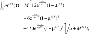where a = B₀/Em.

The first term, , decreases exponentially with time, and the second term, M^3/4t, increases linearly with time, that is, as time, t, increases, the first term becomes negligible quickly when compared with the second term. So, the integral approximately equals M^3/4t.

References

- 1.Barker DJP, editor. Fetal and Infant Origins of Adult Disease. London: BMJ Publishing; 1992. [Google Scholar]
- 2.Barker DJP. Fetal and infant origins of adult disease. Monatsschr Kinderheilkd. 2001;149:S2–S6. [Google Scholar]
- 3.Morley R. Fetal origins of adult disease. Semin Fetal Neonatal Med. 2006;11:73–78. doi: 10.1016/j.siny.2005.11.001. [DOI] [PubMed] [Google Scholar]
- 4.McMillen IC, Robinson JS. Developmental origins of the metabolic syndrome: prediction, plasticity, and programming. Physiol Rev. 2005;85:571–633. doi: 10.1152/physrev.00053.2003. [DOI] [PubMed] [Google Scholar]
- 5.Barker DJP. Fetal origins of coronary heart-disease. Br Med J. 1995;311:171–174. doi: 10.1136/bmj.311.6998.171. [DOI] [PMC free article] [PubMed] [Google Scholar]
- 6.Barker DJP, Osmond D, Winter PD, Margetts B, Simmonds SJ. Weight in infancy and death from ischaemic heart disease. Lancet. 1989;2:577–580. doi: 10.1016/s0140-6736(89)90710-1. [DOI] [PubMed] [Google Scholar]
- 7.Soto N, Bazaes RA, Pena V, et al. Insulin sensitivity and secretion are related to catch-up growth in small-for-gestational-age infants at age 1 year: results from a prospective cohort. J Clin Endocr Metab. 2003;88:3645–3650. doi: 10.1210/jc.2002-030031. [DOI] [PubMed] [Google Scholar]
- 8.Simmons RA, Templeton LJ, Gertz SJ. Intrauterine growth retardation leads to the development of type 2 diabetes in the rat. Diabetes. 2001;50:2279–2286. doi: 10.2337/diabetes.50.10.2279. [DOI] [PubMed] [Google Scholar]
- 9.Woodall SM, Johnston BM, Breier BH, Gluckman PD. Chronic maternal undernutrition in the rat leads to delayed postnatal growth and elevated blood pressure of offspring. Pediatr Res. 1996;40:438–443. doi: 10.1203/00006450-199609000-00012. [DOI] [PubMed] [Google Scholar]
- 10.Lucas A, Fewtrell MS, Cole TJ. Education and debate—fetal origins of adult disease—the hypothesis revisited. Br Med J. 1999;319:245–249. doi: 10.1136/bmj.319.7204.245. [DOI] [PMC free article] [PubMed] [Google Scholar]
- 11.Hales CN, Ozanne SE. The dangerous road of catch-up growth. J Physiol (Lond) 2003;547:5–10. doi: 10.1113/jphysiol.2002.024406. [DOI] [PMC free article] [PubMed] [Google Scholar]
- 12.Hales CN, Barker DJP. Type-2 (on-insulin-dependent) diabetes-mellitus—the thrifty phenotype hypothesis. Diabetologia. 1992;35:595–601. doi: 10.1007/BF00400248. [DOI] [PubMed] [Google Scholar]
- 13.Hales CN, Barker DJP. The thrifty phenotype hypothesis. Br Med Bull. 2001;60:5–20. doi: 10.1093/bmb/60.1.5. [DOI] [PubMed] [Google Scholar]
- 14.Barker DJP. Maternal nutrition, fetal nutrition, and disease in later life. Nutrition. 1997;13:807–813. doi: 10.1016/s0899-9007(97)00193-7. [DOI] [PubMed] [Google Scholar]
- 15.Sayer AA, Dunn R, Langley-Evans S, Cooper C. Prenatal exposure to a maternal low protein diet shortens life span in rats. Gerontology. 2001;47:9–14. doi: 10.1159/000052764. [DOI] [PubMed] [Google Scholar]
- 16.Hales CN, Desai M, Ozanne SE, Crowther NJ. Fishing in the stream of diabetes: from measuring insulin to the control of fetal organogenesis. Biochem Soc Trans. 1996;24:341–350. doi: 10.1042/bst0240341. [DOI] [PubMed] [Google Scholar]
- 17.Jennings BJ, Ozanne SE, Dorling MW, Hales CN. Early growth determines longevity in male rats and may be related to telomere shortening in the kidney. Febs Lett. 1999;448:4–8. doi: 10.1016/s0014-5793(99)00336-1. [DOI] [PubMed] [Google Scholar]
- 18.Leon DA, Koupilova I, Lithell HO, et al. Failure to realise growth potential in utero and adult obesity in relation to blood pressure in 50 year old Swedish men. Br Med J. 1996;312:401–406. doi: 10.1136/bmj.312.7028.401. [DOI] [PMC free article] [PubMed] [Google Scholar]
- 19.Eriksson JG, Forsen T, Tuomilehto J, Winter PD, Osmond C, Barker DJP. Catch-up growth in childhood and death from coronary heart disease: longitudinal study. Br Med J. 1999;318:427–431. doi: 10.1136/bmj.318.7181.427. [DOI] [PMC free article] [PubMed] [Google Scholar]
- 20.Ong KKL, Ahmed ML, Emmett PM, Preece MA, Dunger DB, Pregnancy ALS. Association between postnatal catch-up growth and obesity in childhood: prospective cohort study. Br Med J. 2000;320:967–971. doi: 10.1136/bmj.320.7240.967. [DOI] [PMC free article] [PubMed] [Google Scholar]
- 21.Poore KR, Forhead AJ, Gardner DS, Giussani DA, Fowden AL. The effects of birth weight on basal cardiovascular function in pigs at 3 months of age. J Physiol (Lond) 2002;539:969–978. doi: 10.1113/jphysiol.2001.012926. [DOI] [PMC free article] [PubMed] [Google Scholar]
- 22.Langley-Evans SC, Sculley DV. The association between birthweight and longevity in the rat is complex and modulated by maternal protein intake during fetal life. Febs Lett. 2006;580:4150–4153. doi: 10.1016/j.febslet.2006.06.062. [DOI] [PubMed] [Google Scholar]
- 23.Ozanne SE, Hales CN. Lifespan—catch-up growth and obesity in male mice. Nature. 2004;427:411–412. doi: 10.1038/427411b. [DOI] [PubMed] [Google Scholar]
- 24.Martin-Gronert MS, Tarry-Adkins JL, Cripps RL, Chen JH, Ozanne SE. Maternal protein restriction leads to early life alterations in the expression of key molecules involved in the aging process in rat offspring. Am J Physiol Regul Integr Comp Physiol. 2008;294:R494–R500. doi: 10.1152/ajpregu.00530.2007. [DOI] [PubMed] [Google Scholar]
- 25.Metcalfe NB, Monaghan P. Compensation for a bad start: grow now, pay later? Trends Ecol Evol. 2001;16:254–260. doi: 10.1016/s0169-5347(01)02124-3. [DOI] [PubMed] [Google Scholar]
- 26.Gluckman PD, Hanson MA. Developmental origins of disease paradigm: a mechanistic and evolutionary perspective. Pediatr Res. 2004;56:311–317. doi: 10.1203/01.PDR.0000135998.08025.FB. [DOI] [PubMed] [Google Scholar]
- 27.Saul N, Pietsch K, Menzel R, Stürzenbaum SR, Steinberg CEW. The longevity effect of tannic acid in Caenorhabditis elegans: disposable soma meets hormesis. J Gerontol A Biol Sci Med Sci. 2010;65A:626–635. doi: 10.1093/gerona/glq051. [DOI] [PubMed] [Google Scholar]
- 28.Koziel S, Jankowska EA. Effect of low versus normal birthweight on menarche in 14-year-old Polish girls. J Paediatr Child Health. 2002;38:268–271. doi: 10.1046/j.1440-1754.2002.00793.x. [DOI] [PubMed] [Google Scholar]
- 29.Hoy WE, Rees M, Kile E, Mathews JD, Wang ZQ. A new dimension to the Barker hypothesis: low birthweight and susceptibility to renal disease. Kidney Int. 1999;56:1072–1077. doi: 10.1046/j.1523-1755.1999.00633.x. [DOI] [PubMed] [Google Scholar]
- 30.Kajantie E, Osmond C, Barker DJP, Forsen T, Phillips DIW, Eriksson JG. Size at birth as a predictor of mortality in adulthood: a follow-up of 350 000 person-years. Int J Epidemiol. 2005;34:655–663. doi: 10.1093/ije/dyi048. [DOI] [PubMed] [Google Scholar]
- 31.Harding JE. The nutritional basis of the fetal origins of adult disease. Int J Epidemiol. 2001;30:15–23. doi: 10.1093/ije/30.1.15. [DOI] [PubMed] [Google Scholar]
- 32.Rose MR. The Evolutionary Biology of Aging. Oxford: Oxford University Press; 1991. [Google Scholar]
- 33.Williams G. Pleiotropy, natural selection, and the evolution of senescence. Evolution. 1957;11:398–411. [Google Scholar]
- 34.Kirkwood TBL. The disposable soma theory of aging. In: Harrison DE, editor. Genetic Effects on Aging II. Caldwell, NJ: Telford Press; 1990. pp. 9–19. [Google Scholar]
- 35.Bergman A, Atzmon G, Ye K, MacCarthy T, Barzilai N. Buffering mechanisms in aging: a systems approach toward uncovering the genetic component of aging. PLoS Comp Biol. 2007;3:e170. doi: 10.1371/journal.pcbi.0030170. [DOI] [PMC free article] [PubMed] [Google Scholar]
- 36.Barja G. Aging in vertebrates, and the effect of caloric restriction: a mitochondrial free radical production-DNA damage mechanism? Biol Rev. 2004;79:235–251. doi: 10.1017/s1464793103006213. [DOI] [PubMed] [Google Scholar]
- 37.Van Remmen H, Jones DP. Current thoughts on the role of mitochondria and free radicals in the biology of aging. J Gerontol A Biol Sci Med Sci. 2009;64A:171–174. doi: 10.1093/gerona/gln058. [DOI] [PMC free article] [PubMed] [Google Scholar]
- 38.Sierra F. Is (your cellular response to) stress killing you? J Gerontol A Biol Sci Med Sci. 2006;61:557–561. doi: 10.1093/gerona/61.6.557. [DOI] [PubMed] [Google Scholar]
- 39.Campisi J, Vijg J. Does damage to DNA and other macromolecules play a role in aging? If so, how? J Gerontol A Biol Sci Med Sci. 2009;64A:175–178. doi: 10.1093/gerona/gln065. [DOI] [PMC free article] [PubMed] [Google Scholar]
- 40.Hulbert AJ, Pamplona R, Buffenstein R, Buttemer WA. Life and death: metabolic rate, membrane composition, and life span of animals. Physiol Rev. 2007;87:1175–1213. doi: 10.1152/physrev.00047.2006. [DOI] [PubMed] [Google Scholar]
- 41.Lombard DB, Chua KF, Mostoslavsky R, France S, Gostissa M, Alt FW. DNA repair, genome stability, and aging. Cell. 2005;120:497–512. doi: 10.1016/j.cell.2005.01.028. [DOI] [PubMed] [Google Scholar]
- 42.Balaban RS, Nemoto S, Finkel T. Mitochondria, oxidants, and aging. Cell. 2005;120:483–495. doi: 10.1016/j.cell.2005.02.001. [DOI] [PubMed] [Google Scholar]
- 43.Harper ME, Bevilacqua L, Hagopian K, Weindruch R, Ramsey JJ. Ageing, oxidative stress, and mitochondrial uncoupling. Acta Physiol Scand. 2004;182:321–331. doi: 10.1111/j.1365-201X.2004.01370.x. [DOI] [PubMed] [Google Scholar]
- 44.Burton GJ, Hempstock J, Jauniaux E. Oxygen, early embryonic metabolism and free radical-mediated embryopathies. Reprod Biomed Online. 2003;6:84–96. doi: 10.1016/s1472-6483(10)62060-3. [DOI] [PubMed] [Google Scholar]
- 45.Burton GJ, Jauniaux E. Placental oxidative stress: from miscarriage to preeclampsia. J Soc Gynecol Invest. 2004;11:342–352. doi: 10.1016/j.jsgi.2004.03.003. [DOI] [PubMed] [Google Scholar]
- 46.West GB, Brown JH, Enquist BJ. A general model for ontogenetic growth. Nature. 2001;413:628–631. doi: 10.1038/35098076. [DOI] [PubMed] [Google Scholar]
- 47.Brody S. Bioenergetics and Growth. Darien, CT: Hafner; 1964. [Google Scholar]
- 48.Hou C, Zuo WY, Moses ME, Woodruff WH, Brown JH, West GB. Energy uptake and allocation during ontogeny. Science. 2008;322:736–739. doi: 10.1126/science.1162302. [DOI] [PMC free article] [PubMed] [Google Scholar]
- 49.Moses ME, Hou C, Woodruff WH, et al. Revisiting a model of ontogenetic growth: estimating model parameters from theory and data. Am Nat. 2008;171:632–645. doi: 10.1086/587073. [DOI] [PubMed] [Google Scholar]
- 50.Zuo WY, Moses ME, Hou C, Woodruff WH, West GB, Brown JH. Response to comments on “energy uptake and allocation during ontogeny. Science. 2009;325:1206-c. doi: 10.1126/science.1162302. [DOI] [PMC free article] [PubMed] [Google Scholar]
- 51.Ricklefs RE. Embryo growth rates in birds and mammals. Funct Ecol. 2010;24:588–596. [Google Scholar]
- 52.Morowitz HJ. Foundations of Bioenergetics. New York: Academic Press; 1978. [Google Scholar]
- 53.Calow P. Conversion efficiencies in heterotrophic organisms. Biol Rev. 1977;52:385–409. [Google Scholar]
- 54.Withers PC. Comparative Animal Physiology. Fort Worth, TX: Saunders College/Harcourt College; 1992. [Google Scholar]
- 55.Peters RH. The Ecological Implications of Body Size. New York: Cambridge University Press; 1986. [Google Scholar]
- 56.Needham J. Chemical Embryology. New York: Macmillan; 1931. [Google Scholar]
- 57.McCoy MW, Gillooly JF. Predicting natural mortality rates of plants and animals. Ecol Lett. 2008;11:710–716. doi: 10.1111/j.1461-0248.2008.01190.x. [DOI] [PubMed] [Google Scholar]
- 58.Gaillard JM, Loison A, Festa-Bianchet M, Yoccoz NG, Solberg E. Ecological correlates of life span in populations of large herbivorous mammals. Popul Dev Rev. 2003;29:39–56. [Google Scholar]
- 59.Speakman JR. Body size, energy metabolism and lifespan. J Exp Biol. 2005;208:1717–30. doi: 10.1242/jeb.01556. [DOI] [PubMed] [Google Scholar]
- 60.Kirkwood TB, Holliday R. The evolution of ageing and longevity. Proc R Soc Biol B. 1979;205:531–546. doi: 10.1098/rspb.1979.0083. [DOI] [PubMed] [Google Scholar]
- 61.Gluckman PD, Hanson MA. The developmental origins of the metabolic syndrome. Trends Endocrin Met. 2004;15:183–187. doi: 10.1016/j.tem.2004.03.002. [DOI] [PubMed] [Google Scholar]
- 62.Lehninger AL, Nelson DL, Cox MM. Principles of Biochemistry. New York: Worth Publishers; 1993. [Google Scholar]