Model-based feature construction for multivariate decoding

Abstract

Conventional decoding methods in neuroscience aim to predict discrete brain states from multivariate correlates of neural activity. This approach faces two important challenges. First, a small number of examples are typically represented by a much larger number of features, making it hard to select the few informative features that allow for accurate predictions. Second, accuracy estimates and information maps often remain descriptive and can be hard to interpret. In this paper, we propose a model-based decoding approach that addresses both challenges from a new angle. Our method involves (i) inverting a dynamic causal model of neurophysiological data in a trial-by-trial fashion; (ii) training and testing a discriminative classifier on a strongly reduced feature space derived from trial-wise estimates of the model parameters; and (iii) reconstructing the separating hyperplane. Since the approach is model-based, it provides a principled dimensionality reduction of the feature space; in addition, if the model is neurobiologically plausible, decoding results may offer a mechanistically meaningful interpretation. The proposed method can be used in conjunction with a variety of modelling approaches and brain data, and supports decoding of either trial or subject labels. Moreover, it can supplement evidence-based approaches for model-based decoding and enable structural model selection in cases where Bayesian model selection cannot be applied. Here, we illustrate its application using dynamic causal modelling (DCM) of electrophysiological recordings in rodents. We demonstrate that the approach achieves significant above-chance performance and, at the same time, allows for a neurobiological interpretation of the results.

1 INTRODUCTION

How does the central nervous system represent information about sensory stimuli, cognitive states, and behavioural outputs? Recent years have witnessed an enormous increase in research that addresses the encoding problem from an inverse perspective: by asking whether we can decode information from brain activity alone. Rather than predicting neural activity in response to a particular stimulus, the decoding problem is concerned with how much information about a stimulus can be deciphered from measurements of neural activity.

The vast majority of recent decoding studies are based on functional magnetic resonance imaging (fMRI). An increasingly popular approach has been to relate multivariate single-trial data to a particular perceptual or mental state. The technique relies on applying algorithms for pattern classification to fMRI data. A classification algorithm is first trained on data from a set of trials with known labels (e.g., stimulus A vs. stimulus B). It is then tested on a set of trials without labels. Comparing the predicted labels with the true labels results in a measure of classification accuracy, which in turn serves as an estimate of the algorithm’s generalization performance. Successful above-chance classification provides evidence that information about the type of trial (e.g., the type of stimulus) can indeed be decoded from single-trial volumes of data.¹

Challenges for current decoding methods

There are two key challenges for current decoding methods. The first challenge is concerned with the problem of feature selection. In the case of fMRI, for instance, a whole-brain scan may easily contain around 300,000 voxels, whereas the number of experimental repetitions (i.e., trials) is usually on the order of tens. This mismatch requires carefully designed algorithms for reducing the dimensionality of the feature space without averaging out informative activity. Since an exhaustive search of the entire space of feature subsets is statistically unwarranted and computationally intractable, various heuristics have been proposed. One common approach, for example, is to simply include only those voxels whose activity, when considered by itself, significantly differs between trial types within the training set (Cox & Savoy, 2003). This type of univariate feature selection is computationally efficient, but it fails to find voxels that only reveal information when considered as an ensemble. Another method, termed searchlight analysis, finds those voxels whose local environment allows for above-chance classification (Kriegeskorte, Goebel, & Bandettini, 2006). Unlike the first approach, searchlight feature selection is multivariate, but it fails to detect more widely distributed sets of voxels that jointly encode information about the variable of interest. The key question in feature selection is: how can we find a feature space that is both informative and constructable in a biologically meaningful way?

The second challenge for current decoding methods is the problem of meaningful inference. Classification algorithms per se yield predictions, in the sense of establishing a statistical relationship between (multivariate) neural activity and a (univariate) variable of interest. The ability to make predictions is indeed the primary goal in fields concerned with the design of brain-machine interfaces (Sitaram et al., 2007), novel tools for phenomenological clinical diagnosis (e.g., Ford et al., 2003), or algorithms for lie detection (Davatzikos et al., 2005; Kozel et al., 2005; Bles & Haynes, 2008; Krajbich, Camerer, Ledyard, & Rangel, 2009). A researcher interested in prediction puts all effort into the design of algorithms that maximize classification accuracy. The goal of cognitive neuroscience, by contrast, is a different one. Here, instead of merely maximizing prediction accuracy, the aim is to make inferences on structure-function mappings in the brain. High prediction accuracy is not a goal in itself but is used as a measure of the amount of information that can be extracted from neural activity (cf. Friston et al., 2008). Yet, there are limits on what conclusions can be drawn from this approach. To what extent, for instance, can we claim to have deciphered the neural code when we have designed an algorithm that can tell apart two discrete types of brain state? How much have we learned about how the brain encodes information if the algorithm tells us, for example, that two cognitive states are distinguished by complicated spatial patterns of voxels? This is what we refer to as the challenge of meaningful inference: how can we design a decoding algorithm that allows us to interpret its results with reference to the mechanisms of the underlying biological system?

In order to address the first challenge, the problem of feature selection, the vast majority of decoding methods resort to heuristics. Popular strategies include: selecting voxels based on an anatomical mask (e.g., Haynes & Rees, 2005; Kamitani & Tong, 2005) or a functional localizer (e.g., Cox & Savoy, 2003; Serences & Boynton, 2007); combining voxels into supervoxels (e.g., Davatzikos et al., 2005); finding individually-informative voxels in each cross-validation fold using a general linear model (e.g., Krajbich, Camerer, Ledyard, & Rangel, 2009) or a searchlight analysis (e.g., Kriegeskorte, Goebel, & Bandettini, 2006; Haynes et al., 2007); or reducing the dimensionality of the feature space in an unsupervised fashion (e.g., by applying a Principal Component Analysis, see Mourao-Miranda, Bokde, Born, Hampel, & Stetter, 2005). Other recently proposed strategies include automatic relevance determination (Yamashita, Sato, Yoshioka, Tong, & Kamitani, 2008) and classification with a built-in sparsity constraint (e.g., Grosenick, Greer, & Knutson, 2008; van Gerven, Hesse, Jensen, & Heskes, 2009). However, most of these methods are only loosely constrained by rules of biological plausibility. Notable exceptions are approaches that attempt to account for the inherent spatial structure of the feature space (Kriegeskorte et al., 2006; Soon, Namburi, Goh, Chee, & Haynes, 2009; Grosenick, Klingenberg, Greer, Taylor, & Knutson, 2009) or that use a model to identify a particular stimulus identity (e.g., Kay, Naselaris, Prenger, & Gallant, 2008; Mitchell et al., 2008; Formisano, De Martino, Bonte, & Goebel, 2009). However, conventional methods for feature selection may easily lead to rather arbitrary subsets of selected voxels—deemed informative by the classifier, yet not trivial to interpret physiologically.

Facing the second challenge, the problem of meaningful inference, most decoding studies to date draw conclusions from classification accuracies themselves. Such approaches can be grouped into: (i) pattern discrimination: can two types of trial be distinguished? (e.g., Mitchell et al., 2003; Ford et al., 2003); (ii) spatial pattern localization: where in the brain is discriminative information encoded? (e.g., Kamitani & Tong, 2005, 2006; Haynes & Rees, 2005; Hampton & O’Doherty, 2007; Kriegeskorte, Formisano, Sorger, & Goebel, 2007; Grosenick, Greer, & Knutson, 2008; Hassabis et al., 2009; Howard, Plailly, Grueschow, Haynes, & Gottfried, 2009); and (iii) temporal pattern localization: when does specific information become available to a brain region? (e.g., Polyn, Natu, Cohen, & Norman, 2005; Grosenick et al., 2008; Bode & Haynes, 2009; Harrison & Tong, 2009; Soon et al., 2009). Yet, mechanistic conclusions that relate to biologically meaningful entities such as brain connectivity or synaptic plasticity are hard to draw. Conventional classifiers allow for the construction of information maps, but these are usually difficult to relate to concrete neurophysiological or biophysical mechanisms.

Decoding with model-based feature construction

In order to address the limitations outlined above, we propose a new scheme which we refer to as decoding with model-based feature construction (see Figure 1). The approach comprises three steps. First, a biologically informed model is constructed that describes the dynamics of neural activity underlying the observed measurements. This model explicitly incorporates prior knowledge about biophysical and biological mechanisms but does not contain any representation of the class labels or cognitive states that are to be classified. Next, units of classification are formed, and the model is fitted to the measured data for each unit separately. Typically, a unit of classification corresponds either to an individual trial (leading to trial-by-trial decoding) or to an individual subject (leading to subject-by-subject classification). Crucially, the model is designed to accommodate observations gathered from all classes, and therefore, when being inverted, it remains oblivious to the class a given unit of data stems from.² In the second step of our approach, a classification algorithm is trained and tested on the data. Crucially, the only features submitted to the algorithm are parameter estimates provided by model inversion, e.g., posterior means.³ Third, the weights are reconstructed that the classifier has assigned to individual features. This approach yields both an overall classification accuracy and a set of feature weights. They can be interpreted, respectively, as the degree to which the biologically informed model has captured differences between classes, and the degree to which biophysical model parameters have proven informative (in the context of all features considered) in distinguishing between these classes. A full description of all three steps will be provided in Section 2.

Fig. 1. Model-based feature construction.

A decoding analysis starts off by forming units of classification (e.g., individual trials) and splitting up the data into a training set and a test set. Each example, represented by a vector, carries a class label (e.g., A or B). Feature construction (or feature selection) is the process of mapping a high-dimensional input space onto a lower-dimensional feature space so that examples can be represented by more compact descriptions. The same feature construction that was used on the training data is applied to the test data. The actual classification algorithm then makes use of the information from the training set to predict the unknown labels of the test examples. Comparing predicted labels with true labels yields a measure of classification accuracy. Conventional feature construction (left trapezium) often relies on generic methods for dimensionality reduction (see Section 1). Model-based feature construction, by contrast (right trapezium), rests on a mechanistically interpretable model of how the observed data were generated by underlying neuronal processes. This model is inverted separately for each example, and the resulting parameter estimates constitute the feature space. Thus, the resulting feature weights can be interpreted in relation to the underlying model, and accuracies can be used for model comparison.

When interpreting feature weights one should keep in mind that features with large weights are informative (with regard to discriminating trial or subject labels) when considered as part of an ensemble of features. Importantly, a non-zero feature weight does not necessarily imply that this feature is informative by itself (i.e., if it were used in isolation for classification). For example, a feature may be useless by itself but become useful when considered jointly with others (c.f. Figure 2a). A nice example of how this situation may occur in practice has been described in Blankertz, Lemm, Treder, Haufe, & Müller (2010). Hence, one should not interpret model-based feature weights in isolation but in the context of the set of model parameters considered.

Fig. 2. Class separability in feature space.

(a) Two features may jointly encode class information when they hardly allow for class separation on their own. The plot shows synthetic data in a two-dimensional feature space (points) along with their class-conditional density functions (areas). Even though the class-conditional distributions overlap heavily along both dimensions, a classifier can easily separate the classes using a diagonal hyperplane. (b) Averaging examples within classes may eliminate both noise and signal. The plot illustrates a situation where the distribution of one class is bimodal. The two class-conditional means would coincide in the centre and would be hard to distinguish, whereas a nonlinear classifier can easily tell the two classes apart.

The idea of analysing the role of parameters may seem very similar to standard model-based inference, for instance, when fitting a dynamic causal model to all data from either trial type, and then testing hypotheses about significant parameter differences across trials. However, reconstructing a vector of feature weights in which each feature corresponds to a model parameter provides two additional benefits. First, as described above, feature weights may be sensitive to parameters that do not encode discriminative information on their own but prove valuable for class separation when considered as an ensemble (see Figure 2a). Second, when using a nonlinear kernel, feature weights are sensitive to parameters that allow for class separation even when classes are not linearly separable. This effect can be observed, for example, when classes are non-contiguous: trials of one type might be characterized by a parameter value that is either low or high while the same parameter lies in a medium range for trials of the other type (see Figure 2b).

Decoding with model-based feature construction has three potential advantages over previous methods. First, it rests upon a principled and biologically informed way of generating a feature space. Second, decoding results can be interpreted in the context of a mechanistic model. Third, our approach may supplement evidence-based approaches, such as Bayesian model selection (BMS) for DCM, in two ways: (i) it enables model-based decoding when discriminability of trials or subjects is not afforded by differences in model structure, but only by patterns of parameter estimates under the same model structure, and (ii) it enables structural model selection in cases where BMS for current implementations of DCM is not applicable. We deal with these points in more depth in the Discussion.

Proof of concept

Model-based feature spaces can be constructed for various acquisition modalities, including fMRI, electroencephalography (EEG), magnetoencephalography (MEG), or electrophysiology. Here, as a proof of principle, we illustrate the applicability of our approach in two independent datasets consisting of electrophysiological recordings from rat cortex. The first dataset is based on a simple whisker stimulation experiment; the second dataset is an auditory mismatch-negativity (MMN) paradigm. In both cases, the aim of decoding is to predict, based on single-trial neural activity, which type of stimulus was administered on each trial.

In both datasets, we construct a feature space on the basis of dynamic causal modelling (DCM), noting that, in principle, any other modelling approach providing trial-by-trial estimates could have been used instead. DCM was originally introduced for fMRI data (Friston et al. 2003) but has subsequently been implemented for a variety of measurement types, such as event-related potentials or spectral densities obtained from electrophysiological measurements (David et al., 2006; Kiebel, Garrido, Rosalyn Moran, Chen, & Friston, 2009; Moran et al., 2009). It views the brain as a nonlinear dynamical system that is subject to external inputs (such as experimental perturbations). Specifically, DCM describes how the dynamics within interconnected populations of neurons evolve over time and how their interactions change as a function of external inputs. Here we apply DCM to electrophysiological recordings, which are highly resolved in time (here: 1 kHz). This makes it possible to fit a neurobiologically inspired network model to individual experimental trials and hence construct a model-based feature space for classification. In order to facilitate the comparison of our scheme with future approaches, our data will be made available online.⁴

2 METHODS

Model-based feature construction can be thought of in terms of three conceptual steps: trial-by-trial estimation of a model (Section 2.1), classification in parameter space (Section 2.2), and reconstruction of feature weights (Section 2.3). The approach could be used with various biological modelling techniques or experimental modalities. Here, we propose one concrete implementation. It is based on trial-by-trial dynamic causal modelling in conjunction with electrophysiology.

2.1 Trial-by-trial dynamic causal modelling

Introduction to DCM

Dynamic causal modelling (DCM) is a modelling approach designed to estimate activity and effective connectivity in a network of interconnected populations of neurons (Friston, Harrison, & Penny, 2003). DCM regards the brain as a nonlinear dynamic system of interconnected nodes, and an experiment as a designed perturbation of the system’s dynamics. Regardless of data modality, dynamic causal models are generally hierarchical, comprising two model layers (Stephan et al., 2007): first, a model of neuronal population dynamics that includes neurobiologically meaningful parameters such as synaptic weights and their context-specific modulation, spike-frequency adaptation, or conduction delays; second, a modality-specific forward model that translates source activity into measurable observations. It is the neuronal model that is typically of primary interest.

For a given set of recorded data, estimating the parameters of a dynamic causal model means inferring what neural causes will most likely have given rise to the observed responses, conditional on the model. Such models can be applied to a single population of neurons, e.g., a cortical column, to make inferences about neurophysiological processes such as amplitudes of postsynaptic responses or spike-frequency adaptation (Moran et al., 2008). More frequently, however, it is used to investigate the effective connectivity among remote regions and how it changes with experimental context (e.g., Garrido et al., 2008; Stephan et al., 2008). In this paper, we will use DCM in both ways, applying it to two separate datasets, one single-site recording from the somatosensory barrel cortex and a two-electrode recording from the auditory cortex.

There are two reasons why dynamic causal modelling is a particularly promising basis for model-based feature construction. First, all model constituents mimic neurobiological mechanisms and hence have an explicit neuronal interpretation. In particular, the neural-mass model embodied by DCM is largely based on the mechanistic model of cortical columns originally proposed by Jansen & Rit (1995) and further refined in subsequent papers (David & Friston, 2003; David et al., 2006; Moran et al., 2009). Bayesian priors on its biophysical parameters can be updated in light of new experimental evidence (cf. Stephan, Weiskopf, Drysdale, Robinson, & Friston, 2007). In this regard, DCM fundamentally departs from those previous approaches that either characterized experimental effects in a purely phenomenological fashion or were only loosely coupled with biophysical mechanisms. As will be discussed in more detail in Section 2.3, a neuronally plausible model is a key requirement for meaningful model-based decoding results.

The second reason why we chose DCM to illustrate model-based feature construction is that its implementation for electrophysiological data, for example local field potentials (LFP), makes it possible to construct models of measured brain responses without specifying which particular experimental condition was perturbing the system on a given trial.⁵ While DCM is usually employed to explain experimental effects in terms of context-specific modulation of coupling among regions, it is perfectly possible to construct a DCM for LFPs that is oblivious to the type of experimental input which perturbed the system on a given trial. This is an important prerequisite for the applicability of the model to stimulus decoding: when we wish to predict, for a given trial, which stimulus was presented to the brain, based on a model-induced feature space, the model must not have any knowledge of the stimulus identity in the first place.

DCM for LFPs

We illustrate model-based feature construction applying a dynamic causal model for evoked responses to data from electrophysiological recordings in rats. A detailed description of this model can be found in other publications (David & Friston, 2003; Kiebel et al., 2009; Moran et al., 2008; Moran et al., 2009). However, in order to keep the present paper self-contained, a brief summary of the main modelling principles is presented in the following section.

The neural-mass model

The neural-mass model in DCM represents the bottom layer within the hierarchy. It describes a set of n neuronal populations (characterized by m states each) as a system of interacting elements, and it models their dynamics in the context of experimental perturbations. At each time point t, the state of the system is expressed by a vector $\mathit{x}\left(t\right)\in {\mathbb{R}}^{n\times m}$. The evolution of the system over time is described by a set of delay differential equations that evolve the state vector and account for conduction delays among spatially separate populations. The equations specify the rate of change of activity in each region (i.e., of each element in x(t)) as a function of three variables: the current state x(t) itself, the strength of experimental inputs u(t) (e.g., sensory stimulation), and a set of time-invariant parameters θ. Thus, in general terms, the dynamics of the model are given by an n-valued function $\mathit{F}\left(x\right)=\frac{dx}{dt}$.

Within the framework of DCM, each of the n regions is modelled as a microcircuit whose properties are derived from the biophysical model of cortical columns proposed by Jansen & Rit (1995). Specifically, each region is assumed to comprise three subpopulations of neurons whose voltages and currents constitute the state vector ${\mathit{x}}^{\left(k\right)}\in {\mathbb{R}}^9$ of a region k. These populations comprise pyramidal cells (in supragranular and infragranular layers), excitatory interneurons (granular or spiny stellate cells in the granular layer), and inhibitory interneurons (in supragranular and infragranular layers). The connectivity within a column or region is modelled by intrinsic connections that, depending on the source, can be inhibitory or excitatory. Connections between remote neuronal populations are excitatory (glutamatergic) and target specific neuronal populations, depending on their relative hierarchical position, resulting in lateral, forward and backward connections as defined by standard neuroanatomical classifications (Felleman & Van Essen, 1991). Experimentally controlled sensory inputs affect the granular layer (e.g., thalamic input arriving in layer IV) and are modelled as a mixture of one fast event-related and various slow, temporally dispersed components of activity. Critically, this input is the same for all trial types.

DCM describes the dynamics of each region by a set of region-specific constants and parameters. These comprise (i) time constants G of the intrinsic connections, (ii) time constants and maximum amplitudes of excitatory/inhibitory postsynaptic responses (T_e/T_i, H_e/H_i), and (iii) input parameters which specify the delay and dispersion of inputs arriving in the granular layer. Depending on how the model is implemented, the first two sets of these parameters can be fixed or remain free. In all our analyses, we used priors with means as described by Moran et al. (2009). For the analysis of the first dataset, priors on G and T_i were given infinite precision in order to keep the model as simple as possible. For the second dataset, representing a more subtle process and acquired under less standardized conditions than the first (i.e., awake behaving vs. anaesthetized animals), we chose prior variances on the scaling of $\frac{1}{16}$ and $\frac{1}{8}$, respectively (cf. Moran et al., 2009).

Two additional sets of parameters control connections between regions: (iv) extrinsic connection parameters, which specify the specific coupling strengths between any two regions; and (v) conduction delays, which characterize the temporal properties of these connections.

Forward model

The forward model within DCM describes how (hidden) neuronal activity in individual regions generates (observed) measurements. In the context of model-based feature construction we are not primarily interested in the parameter space of the forward model. Thus, DCM for LFPs is a natural choice. Compared to relatively complex forward models such as those used for fMRI or EEG, its forward model is simpler, requiring only a single (gain) parameter for approximating the spatial propagation of electrical fields in cortex (Moran et al., 2009). For each region, the model represents field potentials as a mixture of activity in three local neuronal populations: excitatory pyramidal cells (60%); inhibitory interneurons (20%); and spiny stellate (or granular) cells (20%).

Trial-by-trial model estimation

In most applications of dynamic causal modelling, one or several candidate models are fitted to all data from each experimental condition (e.g., by concatenating the averages of all trials from all conditions and providing modulatory inputs that allow for changes in connection strength across conditions). When constructing a model-based feature space, by contrast, we are fitting the model in a true trial-by-trial fashion. It is therefore critical that the model is not aware of the category a given trial was taken from. Instead, its inherent biophysical parameters need to be able to reflect different classes of trials by themselves.

The idea of trial-by-trial model inversion is to estimate, for each trial, the posterior distribution of the parameters given the data. Biologically informed constraints on these parameters (Friston et al., 2003) can be expressed in terms of a prior density p(θ). This prior is combined with the likelihood p(y|θ, λ) to form the posterior density p(θ|y, λ) p(y|θ, λ)p(θ). This inversion can be carried out efficiently by maximizing a variational approximation to ln p(y|m), the log model evidence for a given model m (Friston, Mattout, Trujillo-Barreto, Ashburner, & Penny, 2007). Using a Laplace approximation, this variational Bayes scheme yields a posterior distribution of the parameters in parametric form. Given d parameters, we obtain, for each trial, a vector of posterior means $\widehat{\theta }\in {\mathbb{R}}^d$ and a full covariance matrix $\widehat{\mathrm{C}}\in {\mathbb{R}}^d\times {\mathbb{R}}^d$.

Designing the feature space

Trial-by-trial inversion of the model leads to two sets of conditional posterior densities, (i) for intrinsic parameters describing the neural dynamics within a region, and (ii) for extrinsic parameters specifying the connectivity between regions. When the model comprises a single region only, the parameter space reduces to the first set of parameters (see Table 1a). By contrast, when the model specifies several regions, the second set of parameters comes into play as well (see Table 1b). The two datasets presented in Section 3 will cover both cases.

In the case of a single-region DCM, one possible feature space can be constructed by including the estimated posterior means of all intrinsic parameters θ. Hence, any given trial k can be turned into an example x_k that is described by a feature vector

$${\mathit{x}}_k=({\mu }_T,{\mu }_H,{\mu }_S^1,{\mu }_S^2,{\mu }_C,{\mu }_R^1,{\mu }_R^2)\in {\mathbb{R}}^7,$$ (2.1)

where, for example, μ_T denotes the estimated mean of the posterior p(T|y_k, m) conditioned on the trial-specific data y_k and the model m (see Table 1a for a description of all parameters). (To keep the notation simple, the trial index k has been omitted in the parameters.) Alternatively, the feature space could be extended to additionally include the posterior variances or even the full posterior covariance matrix, leading to feature vectors ${\mathit{x}}_k\in {\mathbb{R}}^{14}$ or ${\mathit{x}}_k\in {\mathbb{R}}^{35}$, respectively.

In the case of a DCM with multiple regions, the feature space can be augmented by the extrinsic parameters governing the dynamics among regions. Indeed, these variables are usually of primary interest whenever there are several regions with potential causal influences over one another. Again, a trial k could be represented by the posterior means alone,

$${\mathit{x}}_k^{\prime }=(\left[\text{intrinsic parameters of all N regions}\right],A_F,A_B,A_L,D)$$ (2.2)

where A_F, A_B, and A_L are matrices representing inter-regional connection strengths, and D parameterizes the delay of these connections (see Table 1b). Additionally, one could include the posterior variances and covariances. The specific feature spaces proposed in this study will be described in Section 3.

2.2 Classification in parameter space

Decoding a perceptual stimulus or a cognitive state from brain activity is typically formalized as a classification problem. In the case of binary classification, we are given a training set (x_i, y_i) of n examples ${\mathit{x}}_i\in {\mathbb{R}}^d$ along with their corresponding labels y_i {−1, +1}. A learning algorithm attempts to find a discriminant function $f\in \mathcal{F}$ from a hypothesis space $\mathcal{F}$ such that the classifier h(x) = sgn f(x) minimizes the overall loss ${\Sigma }_{i=1}^n\ell (y_i,f\left({\mathit{x}}_i\right))$. The loss function ℓ(y, f(x)) is usually designed to approximate the unknown risk $R\left[f\right]=\mathbb{E}\left[\ell (Y,f(\mathit{X})\right]=\int \ell (Y,f\left(\mathit{X}\right))d\mathbb{P}(\mathit{X},Y)$, where X and Y denote the random variables of which the given examples (x_i, y_i) are realizations.

The classification algorithm we use here is an L₂-norm soft-margin support vector machine (SVM) as given in (2.4). In a leave-one-out cross-validation scheme, the classifier is trained and tested on different partitions of the data, resulting in a cross-validated estimate of its generalization performance. Within each fold, we tune the classifier by means of nested cross-validation on the training set. In the case of a linear kernel, we choose the complexity penalty C using a simple linear search in log₂ space; in the case of nonlinear kernels, we run a grid search over all parameters to find those that minimize the cross-validated empirical misclassification rate on the training set.

There are many ways of measuring the performance of a classifier. In what follows, we are interested in the balanced accuracy b, that is, the mean accuracy obtained on either class,

$$b=\frac{1}{2}\left(\frac{TP}{TP+FN}+\frac{TN}{TN+FP}\right),$$ (2.3)

where TP, FP, TN, and FN are the number of true positives, false positives, true negatives, and false negatives, respectively, in the test set. If the classifier performs equally well on either class, then this term reduces to an ordinary accuracy (number of correct predictions divided by number of predictions); if, however, the ordinary accuracy is high only because the classifier takes advantage of an imbalanced test set, then the balanced accuracy, as desired, will drop to chance. We calculate confidence intervals of the true balanced generalization ability by considering the convolution of two Beta-distributed random variables that correspond to the true accuracies on positive and negative examples, respectively (Brodersen, Ong, Stephan, & Buhmann, under review).

2.3 Reconstruction of feature weights

Some classification algorithms can not only be used to make predictions and obtain an estimate of the generalization error that may be expected on new data. Once trained, some algorithms also indicate which features contribute most to the overall performance attained. In cognitive neuroscience, these feature weights can be of much greater interest than the classification accuracy itself. In contemporary decoding approaches applied to fMRI, for example, features usually represent individual voxels. Consequently, a map of feature weights projected back onto the brain (or, in the case of searchlight procedures, accuracies obtained from local neighbourhoods) may, in principle, reveal which voxels in the brain the classifier found informative (cf. Kriegeskorte et al., 2006). However, this approach is often limited to the degree to which one can overcome the two challenges outlined at the beginning: the problem of feature selection and the problem of meaningful interpretation. Not only is it very difficult to design a classifier that actually manages to learn the feature weights of a whole-brain feature space with a dimensionality of 100,000 voxels; it is also not always clear how the frequently occurring salt-and-pepper information maps should be interpreted.

By contrast, using a feature space of biophysically motivated parameters provides a new perspective on feature weights. Since each parameter is associated with a specific biological role, their weights can be naturally interpreted in the context of the underlying model.

In the case of a soft-margin SVM, reconstruction of the feature weights w is straightforward, especially when features are non-overlapping. Here, we briefly summarize the main principles to highlight issues that are important for model-based feature construction (for further pointers, see Ben-Hur, Ong, Sonnenburg, Schölkopf, & Rätsch, 2008). We begin by considering the optimization problem that the algorithm solves during training:

$$\begin{array}{cc}\hfill {\text{min}}_{\mathit{w},b}& \langle w,w\rangle +C{\Sigma }_{i=1}^n{\xi }_i\hfill \\ \hfill \text{s.t.}& {\xi }_i\ge 1-y_i(\langle \mathit{w},{\mathit{x}}_i\rangle +b)\forall i=1,\dots ,n\hfill \\ \hfill & {\xi }_i\ge 0,\hfill \end{array}$$ (2.4)

where w and b specify the separating hyperplane, ξ_i are the slack variables that relax the inequality constraints to tolerate misclassified examples, and C is the misclassification penalty. The soft-margin minimization problem can be solved by maximizing the corresponding Lagrangian

$$\begin{array}{c}\hfill {\text{max}}_{w,b,\lambda ,\alpha }\mathcal{L}(\mathit{w},b,\lambda ,\alpha )=\frac{1}{2}\langle \mathit{w},\mathit{w}\rangle +C{\Sigma }_{i=1}^n{\xi }_i\hfill \\ \hfill +{\Sigma }_{i=1}^n{\alpha }_i(1-y_i(\langle \mathit{w},{\mathit{x}}_i\rangle +b)-{\xi }_i)+{\lambda }^T(-\xi ).\hfill \end{array}$$ (2.5)

In order to solve the Lagrangian for stationary points, we require its partial derivatives to vanish:

$$\frac{\partial L}{\partial \mathit{w}}=\mathit{w}-{\Sigma }_{i=1}^n{y}_i{\alpha }_i{\mathit{x}}_i=0$$ (2.6)

$$\frac{\partial L}{\partial b}=-{\Sigma }_{i=1}^n{y}_i{\alpha }_i=0$$ (2.7)

Rearranging the first constraint (2.6) shows that the vector of feature weights w can be obtained by summing the products y_iα_ix_i,

$$\mathit{w}={\Sigma }_{i=1}^n{y}_i{\alpha }_i{\mathit{x}}_i$$ (2.8)

where ${\mathit{x}}_i\in {\mathbb{R}}^d$ is the i^th example of the training set, y_i {−1, +1} is its true class label, and $a_i\in \mathbb{R}$ is its support-vector coefficient. More generally, when using a kernel K(x,y) = (x) · (y) with an explicit feature map (x) that translates the original feature space into a new space, the feature weights are given by the d-dimensional vector

$$\mathit{w}={\Sigma }_{i=1}^n{y}_i{\alpha }_i\varphi \left({\mathit{x}}_i\right).$$ (2.9)

For example, in the case of a polynomial kernel of degree p, the kernel function

$$K(\mathit{x},\mathit{y})={(a\langle \mathit{x},\mathit{y}\rangle +b)}^p$$ (2.10)

with real coefficients a and b transforms a d-dimensional variable space into a feature space with

$$d^{\prime }=\left(\begin{array}{c}\hfill d+p\hfill \\ \hfill p\hfill \end{array}\right)-1$$ (2.11)

non-constant dimensions (cf. Shawe-Taylor & Cristianini, 2004). In the case of two-dimensional examples x = (x₁, x₂)^T and a polynomial kernel of degree p = 2, for instance, the resulting explicit feature mapping would be given by ${\varphi }_2{\left(\mathit{x}\right)=(a,\sqrt{2ab}{x}_1,\sqrt{2ab}{x}_2,b{x}_1^2,\sqrt{2}b{x}_1{x}_2,b{x}_2^2)}^{\mathrm{T}}$.

Features constructed in this way do not always provide an intuitive understanding. Even harder to interpret are features resulting from kernels such as radial basis functions (RBF). With these kernels, the transformation from a coordinate-like representation into a similarity relation presents a particular obstacle for assessing the relative contributions of the original features to the classification (cf. Schölkopf & Smola, 2002). In the context of model-based feature construction, we will therefore employ learning machines with linear kernels only. We can then report the importance of a hyperplane component w_q in terms of its normalized value

$$f_q≔\frac{w_q}{{\Sigma }_{j=1}^{d\prime }\mid w_j\mid }\in [-1,1],q=1\dots d^{\prime },$$

such that larger magnitudes correspond to higher discriminative power, and all magnitudes sum to unity.

3 RESULTS

As an initial proof of concept, we illustrate the utility of model-based feature construction for multivariate decoding in the context of two independent electrophysiological datasets obtained in rats. The first dataset is based on a somatosensory stimulation paradigm. Using a single-shank electrode with 16 recording sites, we acquired local field potentials from barrel cortex in anaesthetized rats while on each trial one of two whiskers was stimulated by means of a brief deflection. The goal was to decode from neuronal activity which particular whisker had been stimulated on each trial (Section 3.1). The second dataset was obtained during an auditory oddball paradigm. In this paradigm, two tones with different frequencies were repeatedly played to an awake behaving rat: a frequent standard tone; and an occasional deviant tone. The goal was to decode from neuronal activity obtained from two locations in auditory cortex whether a standard tone or a deviant had been presented on a given trial (Section 3.2).⁶

3.1 Dataset 1 – whisker stimulation

The most commonly investigated question in multivariate decoding is to predict from neuronal activity what type of sensory stimulus was administered on a given experimental trial. In order to investigate the applicability of model-based feature construction to this class of experiments, we analysed LFPs acquired from rats in the context of a simple sensory stimulation paradigm.

Experimental paradigm and data acquisition

Two adjacent whiskers were chosen for stimulation that produced reliable responses at the site of recording (dataset A1: whiskers E₁ and D₃; dataset A2: whiskers C₁ and C₃; datasets A3–A4: whiskers D₃ and β). On each trial, one of these whiskers was stimulated by a brief deflection of a piezo actuator. The experiment comprised 600 trials (see Figure 3).

Fig. 3. Experimental design (dataset 1).

The first experiment is based on a simple whisker-stimulation paradigm. (a) On each trial, after a brief prestimulus period, a brief cosine-wave tactile stimulus is administered to one of two whiskers both of which have been confirmed to produce reliable responses at the site of recording. Each trial lasts 2 s, followed by a jittered inter-trial interval. (b) Stimuli are administered using a piezo actuator for each whisker. Local field potentials are recorded from barrel cortex using a 16-channel silicon probe. (c) A conventional decoding analysis, applied to signals from each channel in turn, reveals a smooth profile of discriminative information across the cortical sheet. For each electrode, the diagram shows the prediction accuracy obtained when using a pattern-recognition algorithm to decode the type of whisker that was stimulated on a given trial (see Section 3.1).

Data were acquired from 3 adult male rats. In one of these, an additional experimental session was carried out after the standard experiment described above. In this additional session, the actuator was very close to the whiskers but did not touch it, serving as a control condition to preclude experimental artifacts from driving decoding performance. After the induction of anaesthesia and surgical preparation, animals were fixated in a stereotactic frame. A multielectrode silicon probe with 16 channels was introduced into the barrel cortex. On each trial, voltage traces were recorded from all 16 sites, approximately spanning all cortical layers (sweep duration 2 s). Local field potentials were extracted by band-pass filtering the data (1-200 Hz). All experimental procedures were approved by the local veterinary authorities (see Supplement S1 for a full description of the methods).

Conventional decoding

Before constructing a model-based feature space for decoding, we carried out two conventional decoding analyses. The purpose of the first analysis was to characterize the temporal specificity with which information could be extracted from raw recordings, whereas the second served as a baseline for subsequent model-based decoding.

We characterized the temporal evolution of information in the signal by training and testing a conventional decoding algorithm on individual time bins. Specifically, we used a nonlinear L₂-norm soft-margin support vector machine (SVM) with a radial basis kernel to obtain a cross-validated estimate of generalization performance at each peristimulus time point (Chang & Lin, 2001). Since it is multivariate, the algorithm can pool information across all 16 channels and may therefore yield above-chance performance even at time points when no channel shows a significant difference between signal and baseline. This phenomenon was found in two out of three datasets (see arrows in Figure 4). Particularly strong decoding performance was found in dataset A2, in which, at the end of the recording window, 800 ms after the application of the stimulus, the trial type could still be revealed from individual time bins with an accuracy of approx. 70%.

Fig. 4. Temporal information mapping (dataset 1).

The evolution of discriminative information over time can be visualized by training and testing a conventional decoding algorithm separately on the data within each peristimulus time bin. Here, time bins were formed by sampling the data at 200 Hz, and all 16 channels were included in the feature space. The black curve represents the balanced accuracy (see Section 2.2) obtained on each time bin (left y-axis). Inset percentages (e.g., 82% in A1) represent peak accuracies. Chance levels along with an uncorrected 95% significance margin are shown as white horizontal lines. Raw recordings have been added as a coloured overlay (right y-axis). Each curve represents, for one particular channel, the difference between the averaged signals from all trials of one class versus the other. The width of a curve indicates the range of 2 standard errors around the mean difference, in μV. Separately for each dataset, raw recordings were rescaled to match the range of classification accuracies, and were plotted on an inverse y-scale, i.e., points above the midline imply a higher voltage under stimulus A than under stimulus B. Minimum and maximum voltage differences are given as inset numbers on the left. As expected, since the significance margins around the chance bar are not corrected for multiple comparisons, even the control dataset occasionally achieves above-chance accuracies (as well as below-chance accuracies). Crucially, the diagram shows that the classifier systematically performs well whenever there is a sufficient signal-to-noise ratio. In addition, high accuracies can be achieved even when no individual channel mean on its own shows a particularly notable difference from its baseline (arrows).

In order to obtain a baseline level for overall classification accuracies, we examined how accurately a conventional decoding approach could tell apart the two trial types (see Figure 5). The algorithm was based on the same linear SVM that we would subsequently train and test on model-based features. Furthermore, both conventional and model-based classification were supplied with the same single-channel time series (channel 3), sampled at 1000 Hz over a [−10, 290] ms peristimulus time interval. Thus using 300 data features, we found a highly significant average above-chance accuracy of 95.4% (p < 0.001) across the experimental data (A1–A3), while no significance was attained in the case of the control (A4).

Fig. 5. Conventional vs. model-based decoding performance (dataset 1).

The diagram shows overall classification accuracies obtained on each dataset, contrasting conventional decoding (blue) with model-based decoding (green). Bars represent balanced accuracies along with 95% confidence intervals of the generalization performance (see Section 2.2). Consistent in both conventional (mean 95.4%) and model-based decoding (mean 83.6%), all accuracies are significantly above chance (p < 0.001) on the experimental datasets (A1–A3). By contrast, neither method attains significance at the 0.05 level on the control dataset in which no physical stimuli were administered (A4). Despite a massively reduced feature space, model-based decoding does not perform much worse than the conventional approach and retains highly significant predictive power in all cases.

Model-based decoding

In order to examine the utility of model-based feature construction in this dataset, we designed a simple dynamic causal model (see Supplement S3 for the full model specification) and used its parameter space to train and test a support vector machine. Since the data were recorded from a single cortical region, the model comprised just one region. For trial-by-trial model inversion we used the recorded signal from electrode channel 3, representing activity in the supragranular layer. Using the trial-by-trial estimates of the posterior means of the neuronal model parameters, we generated a 7-dimensional feature space. We then trained and tested a linear SVM to predict, based on this model-based feature space, the type of stimulus for each trial (see Figure 5). We found high accuracies in all three experimental datasets (average accuracy 83.6%, p < 0.001), whereas prediction performance on the control dataset was not significantly different from chance.

These results showed that although the feature space was reduced by two orders of magnitude (from 300 to 7 features), model-based decoding still achieved convincing classification accuracies, all of which were significantly above chance. We then tested whether the model-based approach would yield feature weights that were neurobiologically interpretable and plausible. In order to estimate these feature weights, we trained our linear SVM on the entire dataset and reconstructed the resulting hyperplane (see equation 2.9). Thus, we obtained an estimate of the relative importance of each DCM parameter in distinguishing the two trial types. These estimates revealed a similar pattern across all three experiments (see Figure 6). Specifically, the parameter encoding the onset of sensory inputs to the cortical population recorded from (R₁) was attributed the strongest discriminative power in all datasets.

Fig. 6. Reconstructed feature weights (dataset 1).

In order to make predictions, a discriminative classifier finds a hyperplane that separates examples from the two types of trial. The components of this hyperplane indicate the joint relative importance of individual features in the algorithm’s success (for parameter descriptions see Table 1a). The diagram shows the normalized value of the hyperplane component (x-axis) for the posterior expectation of each model parameter (y-axis). Feature-weight magnitudes sum to unity, and larger values indicate higher discriminative power (see main text). Consistent across all three experiments, the parameter encoding the stimulus onset (R₁) was attributed the strongest discriminative power.

3.2 Dataset 2 – auditory mismatch negativity potentials

In order to explore the utility of model-based decoding in a second domain, we made an attempt to decode auditory stimuli from neuronal activity in behaving animals, using an oddball protocol that underlies a phenomenon known as auditory mismatch negativity.

Experimental paradigm and data acquisition

In the experiment, a series of tones was played to an awake, behaving animal. The sequence consisted of frequent standard tones and occasional deviant tones of a different frequency (see Figure 7a). Tone frequencies and deviant probabilities were varied across experiments (see Supplement S1). A tone was produced by bandpass-filtered noise of carrier frequencies between 5 and 18 kHz and a length of 50 ms (see Figure 7b). Standard and deviant stimuli were presented pseudo-randomly with deviant probabilities of 0.1 (datasets B1 and B3) and 0.2 (dataset B2). The three datasets comprised 900, 500, and 900 trials, respectively.

Fig. 7. Experimental design (dataset 2).

The second experiment was based on an auditory oddball paradigm. (a) On each trial, the animal was presented either with a standard tone or, less frequently, with a deviant of a different frequency. Tone frequencies and deviant probabilities were varied across experiments (see main text). (b) Each trial lasted 600 ms, with a stimulus onset 90 ms after the beginning of a sweep. Recordings comprised 390 ms in total and were followed by an inter-trial interval of 210 ms. (c) In order to allow for data acquisition in an awake behaving animal, signals were transmitted wirelessly to a high-frequency (HF) receiver. A control unit passed these data on to a storage system where they were time-locked to stimulus triggers. This made it possible for the animal to move freely within a cage in a sound-proof chamber.

For the present analyses we used data that was acquired from 3 animals in a sound-attenuated chamber (cf. Jung et al., 2009). In order to record event-related responses in the awake, unrestrained animal, a telemetric recording system was set up using chronically implanted epidural silverball electrodes above the left auditory cortex. The electrodes were connected to an EEG telemetry transmitter that allowed for wireless data transfer. During the period of data acquisition, rats were awake and placed in a cage that ensured a reasonably constrained variance in the distance between the animal and the speakers (see Figure 7c). All experimental procedures were approved by the local governmental and veterinary authorities (see Supplement S1 for a full description of the methods).

A robust finding in analyses of event-related potentials during the auditory oddball paradigm in humans is that deviant tones, compared to standard ones, lead to a significantly more negative peak between 150-200 ms post-stimulus, the so-called ‘mismatch negativity’ or MM (Näätänen, Tervaniemi, Sussman, Paavilainen, & Winkler, 2001; Garrido, Kilner, Stephan, & Friston, 2009). Although the MMN-literature in rodents is much more heterogeneous and almost exclusively concerned with animals under anaesthesia, the observed difference signals in our data are highly consistent with similar studies in rats (e.g., von der Behrens, Bäuerle, Kössl, & Gaese, 2009), showing a negative deflection at approximately 30 ms and a later positive deflection at 100 ms (shaded overlay in Figure 8).

Fig. 8. Temporal information mapping (dataset 2).

By analogy with Figure 4, the diagram shows the temporal evolution of discriminative information in dataset 2. Time bins were formed by sampling the data from both channels at 1000 Hz. The black curve represents the balanced accuracy obtained on each time bin. The coloured overlay shows, separately for both channels, the mean signal from all deviant trials minus the mean signal from all standard trials. The diagram shows that the most typical situation in which the trial type can be decoded with above-chance accuracy is when at least one channel significantly deviates from its baseline (e.g., grey arrow in B1), though such deviations alone are not always sufficient to explain multivariate classification accuracies.

Conventional decoding

By analogy with Section 3.1, we first ran two conventional decoding analyses. For temporal classification, we used a nonlinear support vector machine with a radial basis function kernel (Chang & Lin, 2001) and characterized the temporal evolution of information in the signal by training and testing the same algorithm on individual time bins. In this initial temporal analysis, above-chance classification reliably coincided with the average difference between signal and baseline (see Figure 8).

In order to obtain baseline performance levels for subsequent model-based decoding, we ran a conventional trial-wise classification analysis based on a powerful polynomial kernel over all time points (see Figure 9). In order to ensure a fair comparison, we supplied the algorithm with precisely the same data as used in the subsequent analysis based on a model-induced feature space (see below). Specifically, each trial was represented by the time series of auditory evoked potentials from both electrodes, sampled at 1000 Hz, over a [−10, 310] ms peristimulus time interval (resulting in 320 features). Across the three datasets we obtained an above-chance average prediction accuracy of 81.2% (p < 0.001).

Fig. 9. Conventional vs. model-based decoding performance (dataset 2).

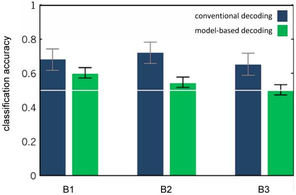
The diagram contrasts conventional decoding (blue) with model-based decoding (green) in terms of overall classification accuracies obtained on each auditory mismatch dataset. Model-based accuracies tend to be lower than conventional accuracies, but they remain significantly above chance in 2 out of 3 cases (59.7% and 54.1%, p < 0.05 each). All results are given in terms of balanced accuracies (see Section 2.2) along with 95% confidence intervals of the generalization performance.

Model-based decoding

In this experiment, data from two electrodes and regions were available, enabling the construction of a two-region DCM. As the exact locations of the electrodes in auditory cortex were not known, we initially evaluated three alternative connectivity layouts between the two regions: (i) a model with forward connections from region 1 to region 2, backward connections from region 2 to region 1, and stimulus input arriving in region 1; (ii) a model with forward connections from region 2 to region 1, backward connections from region 1 to region 2, and stimulus input arriving in region 2; (iii) a model with lateral connections between the two regions and stimulus input arriving in both regions. For each model, we created a 13-dimensional feature space based on the posterior expectations of all neuronal and connectivity parameters. We dealt with the problem of testing multiple hypotheses by splitting the data from all animals into two halves, using the first half of trials for model selection and the second half for reporting decoding results. (Cross-validation across animals, as opposed to within animals, would not provide a sensible alternative here since variability in the location of the electrodes precludes the assumption that all data stem from the same distribution.) Based on the first half of the data within each animal, we found that the best discriminability was afforded by the model that assumes forward connections from region 2 to region 1 and backward connections from region 1 to 2 (see Supplement S3). We then applied this model to the second half of the data, in which the auditory stimulus administered on each trial could be decoded with moderate but highly significant accuracies (p < 0.001) in 2 out of 3 datasets (B1 and B2; see Figure 9).

Feature weights are only meaningful to compute when the classifier performs above chance. Thus, separately for datasets B1 and B2, we trained the same SVM as before on the entire dataset and reconstructed the resulting hyperplane (see equation 2.9). A similar pattern of weights was again found across the datasets (see Figure 10). In particular, the two model parameters with the highest joint discriminative power for both datasets were the parameters representing the strength of the forward and backward connections, respectively (A_F and A_B). Noticeable weights were also assigned to the extrinsic propagation delay (D_1,2) and to the dispersion of the sigmoidal activation function (S₁) (see Figure 10).

Fig. 10. Reconstructed feature weights (dataset 2).

By analogy with Fig. 6, the diagram shows the normalized hyperplane component magnitudes (x-axis) for all model parameters (y-axis). Larger values indicate higher discriminative power when considering the corresponding feature as part of an ensemble of features. One experiment (B3) was excluded from this analysis since its classification accuracy was not significantly above chance (see Figure 9). The sum of the feature weights of the two parameters coding for the )strength of forward and backward connections (parameters A_F and A_B) was highest in both remaining datasets (B1 and B2).

4 DISCUSSION

Recent years have seen a substantial increase in research that investigates the neurophysiological encoding problem from an inverse perspective, asking how well we can decode a discrete state of mind from neuronal activity. However, there are two key challenges that all contemporary methods have to face. First, the problem of feature selection: how do we design a classification algorithm that performs well when most input features are uninformative? Second, the problem of meaningful inference: how should the feature space be designed to allow for a neurobiologically informative interpretation of classification results? In this paper, we have proposed a new approach which we refer to as decoding with model-based feature construction. This approach involves (i) trial-by-trial inversion of a biophysically interpretable model of neural responses, (ii) classification in parameter space, and (iii) interpretation of the ensuing feature weights.

Model-based feature construction addresses the two challenges of feature selection and meaningful interpretation from a new angle. First, the feature space built from conditional estimates of biophysical model parameters has a much lower dimensionality than the raw data, making any heuristics for initial feature-space dimensionality reduction obsolete (see Figure 1). Concerning the second challenge, model-based feature construction offers a new perspective on the interpretation of decoding results. In particular, reconstructing feature weights allows us to deduce which set of biophysical parameters is driving prediction performance. Depending on the formulation of the model, this insight has the potential to enable a mechanistic interpretation of classification results. This advantage may become particularly important in clinical studies where such a model-based classification would have substantial advantages over ‘blind’ classification in that it could convey a pathophysiological interpretation of phenotypic differences between patient groups.

Summary of our findings

In order to demonstrate the utility of the proposed method, we analysed two independent datasets, a multichannel-electrode recording from rat barrel cortex during whisker stimulation under anaesthesia, and a two-electrode recording from two locations in auditory cortex of awake behaving rats during an auditory oddball paradigm. In both datasets, we used a state-of-the-art SVM algorithm in a conventional manner (applying it to approx. 300 ‘raw’ data features, i.e., measured time points) and compared it to a model-based alternative (which reduced the feature space by up to two orders of magnitude). Specifically, we designed a model-based feature space using trial-by-trial DCM; of course, other modelling approaches could be employed instead. Although decoding based on model-based feature construction did not quite achieve the same accuracy as conventional methods, the results were significant in all but one instance. Importantly, it became possible to interpret the resulting feature weights from a neurobiological perspective.

In the analysis of the first dataset, the feature weights revealed a strikingly similar pattern across all three experiments (see Figure 6). In particular, the model parameter representing the onset of sensory inputs to the cortical population recorded from (R₁) made the strongest contribution to the classifier’s discriminative power in all datasets (cf. Table 1). This finding makes sense because in our experiment stimulation of the two whiskers induced differential stimulus input to the single electrode used. For whisker stimulation directly exciting the barrel recorded from, a shorter latency can be expected between sensory stimulus and neuronal response as input is directly received from thalamus. In contrast, for stimulation of the other whisker, afferent activity is expected to be relayed via cortico-cortical connections. Similarly, a stimulus directly exciting the barrel recorded from, should be stronger and less dispersed in time than a stimulus coming from a neighbouring whisker. This is reflected by the finding that the parameters representing stimulus strength (C) and stimulus dispersion (R₂), respectively, were also assigned noticeable classification weights, although not for all three datasets. The pattern of informative features was confirmed in a 2D scatter plot, in which R₁ and R₂ play key roles in delineating the two stimulus classes (see Figure 12 in the Supplement).

In the analysis of the second dataset, the auditory MMN data, a similar pattern of feature weights was again found across the two datasets in which significant classification results had been obtained (Figure 10). This is not a trivial prediction, given that all results are based on entirely independent experiments with inevitable deviations in electrode positions. Nevertheless, several model parameters were found with consistent, non-negligible discriminatory power. These included the strength of the forward and backward connections between the two areas (A_F and A_B) and the dispersion of the sigmoidal activation function (S₁). Other noticeable parameters included the synaptic time constants (T₁ and T₂) and the extrinsic propagation delays (D). These findings are in good agreement with previous studies on the mechanisms of the MMN (e.g., Baldeweg, 2006; Garrido et al., 2008; Kiebel, Garrido, & Friston, 2007). In brief, these earlier studies imply that two separate mechanisms, i.e., predictive coding and adaptation, are likely to contribute to the generation of the MMN. While the latter mechanism relies on changes in postsynaptic responsiveness (which can be modelled through changes in the sigmoidal activation function and/or synaptic time constants), the former highlights the importance of inter-regional connections for conveying information about prediction errors. The results of our model-based classification are consistent with this dual-mechanism view of the MMN.

Optimal decoding

The model-based decoding approach described in this paper employs a biophysically and neurobiologically meaningful model of neuronal interactions to enable a mechanistic interpretation of classification results. This approach departs fundamentally from more generic decoding algorithms that operate on raw data, which may be considered one end of a spectrum of approaches (see Introduction). At the other end lies what is often referred to as optimal decoding.

In optimal decoding, given an encoding model that describes how a cognitive state of interest is represented by a particular neuronal state, the cognitive state can be reconstructed from measured activity by inverting the model. Alternatively, if the correct model is unknown, decoding can be used to compare the validity of different encoding models. Recent examples of this sort include the work by Naselaris et al. (2009) and Miyawaki et al. (2008), who demonstrated the reconstruction of a visual image from brain activity in visual cortex. Other examples include Paninski et al. (2007) and Pillow et al. (2008), who inverted a generalized linear model for spike trains. The power of this approach derives from the fact that it is model-based—if the presumed encoding model is correct, the approach is optimal (cf. Paninski et al., 2007; Pillow et al., 2008; Naselaris et al., 2009; Miyawaki et al., 2008). However, there are two reasons why it does not provide a feasible option in most practical questions of interest.

The first obstacle in optimal decoding is that it requires an encoding model to begin with. In other words, an optimal encoding model requires one to specify exactly and a priori how different cognitive states translate into differential neuronal activity. Putting down such a specification may be conceivable in simple sensory discrimination tasks; but it is not at all clear how one would achieve this in a principled way in the context of more complex paradigms. In contrast, a modelling approach such as DCM for LFPs is agnostic about a prespecified mapping between cognitive states and neuronal states. Instead, it allows one to construct competing models of neuronal responses to external perturbations (e.g., sensory stimuli, or task demands), compare these different hypotheses, select the one with the highest evidence, and use it for the construction of a feature space.

The second problem in optimal decoding is that even when the encoding model is known, its inversion may be computationally intractable. This limitation may sometimes be overcome by restricting the approach to models such as generalized linear models, which have been proposed for spike trains (e.g., Paninski et al., 2007; Pillow et al., 2008); however, such restrictions will only be possible in special cases. It is in these situations where decoding using a model-based feature space could provide a useful alternative.

Choice of classifiers and unit of classification

Decoding with model-based feature construction is compatible with any type of classifier, as long as its design makes it possible to reconstruct feature weights, that is, to estimate the contribution of individual features to the classifier’s success. For example, an SVM with a linear or a polynomial kernel function is compatible with this approach, whereas in other cases (e.g., when using a radial basis function kernel; see Section 2.3), one might have to resort to computationally more expensive alternatives (such as a leave-one-feature-out comparison of overall accuracies).

It should also be noted that feature weights are not independent of the algorithm that was used to learn them. In this study, for example, we illustrated model-based decoding using an SVM. Other classifiers (e.g., a linear discriminant analysis) might differ in determining the separating hyperplane and could thus yield different feature weights. Also, when the analysis goal is not prediction but inference on underlying mechanisms, alternative methods could replace the use of a classifier (e.g., feature-wise statistical testing).

Model-based feature construction may be subject to practical restrictions with regard to the temporal unit of classification. The temporal unit represents the experimental entity that forms an individual example and is associated with an individual label. In most contemporary decoding studies, this is either an experimental trial (trial-by-trial classification) or a subject (subject-by-subject classification; e.g., Ford et al., 2003; Brodersen et al., 2008). Given the high sampling rates and low degrees of serial correlation typically associated with EEG, MEG, or LFP data, DCM can be fitted to individual trials. By contrast, fMRI data have low sampling rates, resulting in only a few data points per trial, and pronounced serial correlations; this makes a piecewise DCM analysis of a trial-wise time series problematic. Thus, decoding with model-based feature construction in the context of fMRI can presently only be used for subject-by-subject classification.

Dynamic and structural model selection

An important aspect in model-based decoding is the choice of a model. For the second dataset described in this paper, for example, there was a natural choice between three different connectivity layouts. The better the model of the neuronal dynamics, the more meaningful the interpretation of the ensuing feature weights should be. But what constitutes a ‘better model’?

Competing models can be evaluated by Bayesian model selection (BMS; Friston et al., 2007; Penny, Stephan, Mechelli, & Friston, 2004; Stephan et al., 2009). In this framework, the best model is the one with the highest (log) model evidence, that is, the highest probability of the data given the model (MacKay, 1992). BMS has been very successful in model-based analyses of neuroimaging and electrophysiological data. It also represents a generic and powerful approach to model-based decoding whenever the trial- or subject-specific class labels can be represented by differences in model structure. However, there are two scenarios in which BMS is problematic and where the approach suggested by this paper may represent a useful alternative.

The first problem is that BMS requires the explananda (i.e., the data features to be explained) to be identical for all competing models. This requirement is fulfilled, for example, for DCMs of EEG or MEG data, where the distribution of potentials or fields at the scalp level does not change with model structure. In this case, BMS enables both dynamic model selection (i.e., concerning the parameterization and mathematical form of the model equations) and structural model selection (i.e., concerning which regions or nodes should be included in the model). However, when dealing with fMRI or invasive recordings, BMS can only be applied if the competing models refer to the same sets of brain regions or neuronal populations; this restriction arises since changing the regions changes the data (Friston, 2009). At present, BMS thus supports dynamic, but not structural, model selection for DCMs of fMRI and invasive recordings. This restriction, however, would disappear once future variants of DCM also optimize spatial parameters of brain activity.

Secondly, with regard to model-based decoding, BMS is limited when the class labels to be discriminated cannot be represented by models of different structure, for example when the differences in neuronal mechanisms operate at a finer conceptual scale than can be represented within the chosen modelling framework. In this case, discriminability of trials (or subjects, respectively) is not afforded by differences in model structure, but may be provided by different patterns of parameter estimates under the same model structure (an empirical example of this case was described recently by Allen et al. (2010)). In other words, differences between trials (or subjects, respectively) can be disclosed by using the parameter estimates of a biologically informed model as summary statistics.

In both above scenarios, the approach proposed in this paper allows for model comparison. This is because model-based feature construction can be viewed as a method for biologically informed dimensionality reduction, and the performance of the classifier is related to how much class information was preserved by the estimates of the model parameters. In other words, training and testing a classifier in a model-induced feature space means that classification accuracies can now be interpreted as the degree to which the underlying model has preserved discriminative information about the features of interest. This view enables a classification-based form of model comparison even when the underlying data (e.g., the chosen regional fMRI time series or electrophysiological recordings) are different, or when the difference between two models lies exclusively in the pattern of parameter estimates.⁷

If discriminability can be afforded by patterns of parameter estimates under the same model structure, one might ask why not simply compare models in which the parameters are allowed to show trial-specific (or subject-specific) differences using conventional model comparison? One can certainly do this, however the nature of the inference is different in a subtle but important way: the differences in evidence between trials (or subjects) afforded by BMS are not the same as the evidence for differences between trials (or subjects). In other words, a difference in evidence is not the same as evidence of difference. This follows from the fact that the evidence is a nonlinear function of the data. This fundamental distinction means that it may be possible to establish significant differences in parameter estimates between trials (or subjects) in the absence of evidence for a model of differences at the within-trial (or within-subject) level. This distinction is related intimately to the difference between random- and fixed-effects analyses. Under this view, the approach proposed in this paper treats model parameters as random effects that are allowed to vary across trials (or subjects); it can thus be regarded as a simple random-effects approach to inference on dynamic causal models.

In summary, our approach is not meant to replace or outperform BMS in situations when it can be applied. In fact, given that BMS rests on computing marginal-likelihood ratios and thus accords with the Neyman-Pearson lemma, one may predict that BMS should be optimally sensitive in situations where it is applicable (for an anecdotal comparison of BMS and model-based decoding, see Supplement S4.) Instead, the purpose of the present paper is to introduce an alternative solution for model comparison in those situations where BMS is not applicable, by invoking a different criterion of comparison: in model-based decoding, the optimal model is the one that generalizes best (in a cross-validation sense) with regard to discriminating trial- or subject-related class labels of interest.

Dimensionality of the feature space

Since it is model based, our approach involves a substantial reduction of the dimensionality of the original feature space. Ironically, depending on the specific scientific question, this reduction may render decoding and cross-validation redundant, since reducing the feature space to a smaller dimensionality may result in having fewer features than observations. In this situation, if one is interested in demonstrating a statistical relationship between the pattern of parameter estimates and class labels, one could use conventional encoding models and eschew the assumptions implicit in cross-validation schemes. In the case of the first dataset, for example, having summarized the trial-specific responses in terms of seven parameter estimates, we could perform multiple linear regression or ANCOVA using the parameter estimates as explanatory variables and the class label as a response variable. In this instance, the ANCOVA parameter estimates reflect the contribution of each model parameter to the discrimination and play the same role as the weights in a classification scheme. In the same vein, we could replace the p-value obtained from a cross-validated accuracy estimate by a p-value based on Hotelling’s T²-test, the multivariate generalization of Student’s t-test. In principle, according to the Neyman-Pearson lemma, this approach should be more sensitive than the cross-validation approach whenever there is a linear relationship between features and class labels. However, in addition to assuming linearity, it depends upon parametric assumptions and a sufficient dimensionality reduction of feature space, which implies that the classification approach has a greater domain of application (for details, see Supplement S5).

An open question is how well our approach scales with an increasing number of model parameters. For example, meaningful interpretation of feature weights might benefit from using a classifier with sparseness properties: while the L₂-norm support vector machine used here, by design, typically leads to many features with small feature weights, other approaches such as sparse nonparametric regression (Caron & Doucet, 2008), sparse linear discriminant analysis (Grosenick et al., 2009), groupwise regularization (van Gerven et al., 2009), or sparse logistic regression (Ryali, Supekar, Abrams, & Menon, 2010) might yield results that enable even better interpretation. One could also attempt to directly estimate the mutual information between the joint distribution of combinations of model parameters and the variable of interest. These questions will be addressed in future studies.

Future applications

In this paper, we have provided a proof-of-concept demonstration for the practical applicability of model-based feature construction. The application domain we have chosen here is the trial-by-trial decoding of distinct sensory stimuli, using evoked potentials recorded from rat cortex. This method may be useful for guiding the formulation of mechanistic hypotheses that can be tested by neurophysiological experiments. For example, if a particular combination of parameters is found to be particularly important for distinguishing between two cognitive or perceptual states, then future experiments could test the prediction that selective impairment of the associated mechanisms should maximally impact on the behavioural expression of those cognitive or perceptual states.

A more important step, from our perspective, however, will be to employ the same approach to subject-by-subject classification on the basis of human fMRI data. This particular domain may hold great potential for clinical applications. In particular, it has been argued that the construction of biologically plausible and mechanistically interpretable models are critical for establishing diagnostic classification schemes that distinguish between pathophysiologically distinct subtypes of spectrum diseases, such as schizophrenia (e.g., Stephan, Friston, & Frith, 2009). The model-based decoding approach as suggested in the present paper could be an important component of this endeavour, particularly in cases where conventional BMS cannot be applied for discrimination of clinical (sub)groups.

REFERENCES

- Allen P, Stephan KE, Mechelli A, Day F, Ward N, Dalton J, Williams SC, et al. Cingulate activity and fronto-temporal connectivity in people with prodromal signs of psychosis. NeuroImage. 2010;49(1):947–955. doi: 10.1016/j.neuroimage.2009.08.038. doi:10.1016/j.neuroimage.2009.08.038. [DOI] [PMC free article] [PubMed] [Google Scholar]
- Baldeweg T. Repetition effects to sounds: evidence for predictive coding in the auditory system. Trends in Cognitive Sciences. 2006;10(3):93–94. doi: 10.1016/j.tics.2006.01.010. doi:10.1016/j.tics.2006.01.010. [DOI] [PubMed] [Google Scholar]
- von der Behrens W, Bäuerle P, Kössl M, Gaese BH. Correlating stimulus-specific adaptation of cortical neurons and local field potentials in the awake rat. The Journal of Neuroscience: The Official Journal of the Society for Neuroscience. 2009;29(44):13837–13849. doi: 10.1523/JNEUROSCI.3475-09.2009. doi:10.1523/JNEUROSCI.3475-09.2009. [DOI] [PMC free article] [PubMed] [Google Scholar]
- Ben-Hur A, Ong CS, Sonnenburg S, Schölkopf B, Rätsch G. Support Vector Machines and Kernels for Computational Biology. PLoS Comput Biol. 2008;4(10):e1000173. doi: 10.1371/journal.pcbi.1000173. doi:10.1371/journal.pcbi.1000173. [DOI] [PMC free article] [PubMed] [Google Scholar]
- Blankertz B, Lemm S, Treder M, Haufe S, Müller K. Single-trial analysis and classification of ERP components - a tutorial. NeuroImage. 2010 doi: 10.1016/j.neuroimage.2010.06.048. in press. [DOI] [PubMed] [Google Scholar]
- Bles M, Haynes J. Detecting concealed information using brain-imaging technology. Neurocase: Case Studies in Neuropsychology, Neuropsychiatry, and Behavioural Neurology. 2008;14(1):82–92. doi: 10.1080/13554790801992784. doi:10.1080/13554790801992784. [DOI] [PubMed] [Google Scholar]
- Bode S, Haynes J. Decoding sequential stages of task preparation in the human brain. NeuroImage. 2009;45(2):606–613. doi: 10.1016/j.neuroimage.2008.11.031. doi:10.1016/j.neuroimage.2008.11.031. [DOI] [PubMed] [Google Scholar]
- Brodersen KH, Ong CS, Stephan KE, Buhmann JM. Posterior distributions of classification accuracy. n.d. under review. [Google Scholar]
- Brodersen KH, Penny WD, Harrison LM, Daunizeau J, Ruff CC, Duzel E, Friston KJ, et al. Integrated Bayesian models of learning and decision making for saccadic eye movements. Neural Networks. 2008;21(9):1247–1260. doi: 10.1016/j.neunet.2008.08.007. doi:10.1016/j.neunet.2008.08.007. [DOI] [PMC free article] [PubMed] [Google Scholar]
- Caron F, Doucet A. Sparse Bayesian nonparametric regression; Proceedings of the 25th international conference on Machine learning; Helsinki, Finland: ACM. 2008; pp. 88–95. doi:10.1145/1390156.1390168. [Google Scholar]
- Chang C, Lin C. LIBSVM: a library for support vector machines. n.d. Retrieved from http://www.csie.ntu.edu.tw/~cjlin/libsvm/
- Cox DD, Savoy RL. Functional magnetic resonance imaging (fMRI) “brain reading”: detecting and classifying distributed patterns of fMRI activity in human visual cortex. NeuroImage. 2003;19(2):261–270. doi: 10.1016/s1053-8119(03)00049-1. doi:10.1016/S1053-8119(03)00049-1. [DOI] [PubMed] [Google Scholar]
- Davatzikos C, Ruparel K, Fan Y, Shen D, Acharyya M, Loughead J, Gur R, et al. Classifying spatial patterns of brain activity with machine learning methods: Application to lie detection. NeuroImage. 2005;28(3):663–668. doi: 10.1016/j.neuroimage.2005.08.009. doi:10.1016/j.neuroimage.2005.08.009. [DOI] [PubMed] [Google Scholar]
- David O, Friston KJ. A neural mass model for MEG/EEG:: coupling and neuronal dynamics. NeuroImage. 2003;20(3):1743–1755. doi: 10.1016/j.neuroimage.2003.07.015. doi:10.1016/j.neuroimage.2003.07.015. [DOI] [PubMed] [Google Scholar]
- David O, Kiebel SJ, Harrison LM, Mattout J, Kilner JM, Friston KJ. Dynamic causal modeling of evoked responses in EEG and MEG. NeuroImage. 2006;30(4):1255–1272. doi: 10.1016/j.neuroimage.2005.10.045. doi:10.1016/j.neuroimage.2005.10.045. [DOI] [PubMed] [Google Scholar]
- Felleman DJ, Van Essen DC. Distributed hierarchical processing in the primate cerebral cortex. Cerebral Cortex (New York, N.Y.: 1991. 1991;1(1):1–47. doi: 10.1093/cercor/1.1.1-a. [DOI] [PubMed] [Google Scholar]
- Ford J, Farid H, Makedon F, Flashman LA, McAllister TW, Megalooikonomou V, Saykin AJ. Medical Image Computing and Computer-Assisted Intervention. MICCAI; 2003. Patient Classification of fMRI Activation Maps; pp. 58–65. Retrieved from http://www.springerlink.com/content/b1fgfpu9reyxw1pu. [Google Scholar]
- Formisano E, De Martino F, Bonte M, Goebel R. “Who” Is Saying “What”? Brain-Based Decoding of Human Voice and Speech. Science. 2009;322(5903):970–973. doi: 10.1126/science.1164318. doi:10.1126/science.1164318. [DOI] [PubMed] [Google Scholar]
- Friston K. Dynamic causal modeling and Granger causality Comments on: The identification of interacting networks in the brain using fMRI: Model selection, causality and deconvolution. NeuroImage. 2009 doi: 10.1016/j.neuroimage.2009.09.031. In Press, Corrected Proof. doi:10.1016/j.neuroimage.2009.09.031. [DOI] [PMC free article] [PubMed] [Google Scholar]
- Friston KJ, Harrison L, Penny W. Dynamic causal modelling. NeuroImage. 2003;19(4):1273–1302. doi: 10.1016/s1053-8119(03)00202-7. doi:10.1016/S1053-8119(03)00202-7. [DOI] [PubMed] [Google Scholar]
- Friston K, Chu C, Mourao-Miranda J, Hulme O, Rees G, Penny W, Ashburner J. Bayesian decoding of brain images. NeuroImage. 2008;39(1):181–205. doi: 10.1016/j.neuroimage.2007.08.013. doi:10.1016/j.neuroimage.2007.08.013. [DOI] [PubMed] [Google Scholar]
- Friston K, Mattout J, Trujillo-Barreto N, Ashburner J, Penny W. Variational free energy and the Laplace approximation. NeuroImage. 2007;34(1):220–234. doi: 10.1016/j.neuroimage.2006.08.035. doi:10.1016/j.neuroimage.2006.08.035. [DOI] [PubMed] [Google Scholar]
- Garrido MI, Friston KJ, Kiebel SJ, Stephan KE, Baldeweg T, Kilner JM. The functional anatomy of the MMN: a DCM study of the roving paradigm. NeuroImage. 2008;42(2):936–944. doi: 10.1016/j.neuroimage.2008.05.018. doi:10.1016/j.neuroimage.2008.05.018. [DOI] [PMC free article] [PubMed] [Google Scholar]
- Garrido MI, Kilner JM, Stephan KE, Friston KJ. The mismatch negativity: a review of underlying mechanisms. Clinical Neurophysiology: Official Journal of the International Federation of Clinical Neurophysiology. 2009;120(3):453–463. doi: 10.1016/j.clinph.2008.11.029. doi:10.1016/j.clinph.2008.11.029. [DOI] [PMC free article] [PubMed] [Google Scholar]
- van Gerven M, Hesse C, Jensen O, Heskes T. Interpreting single trial data using groupwise regularisation. NeuroImage. 2009;46(3):665–676. doi: 10.1016/j.neuroimage.2009.02.041. doi:10.1016/j.neuroimage.2009.02.041. [DOI] [PubMed] [Google Scholar]
- Grosenick L, Greer S, Knutson B. Interpretable classifiers for fMRI improve prediction of purchases. IEEE Transactions on Neural Systems and Rehabilitation Engineering. 2008 doi: 10.1109/TNSRE.2008.926701. Retrieved from http://www-psych.stanford.edu/~span/Publications/lg08tnsre_proof.pdf. [DOI] [PubMed] [Google Scholar]
- Grosenick L, Klingenberg B, Greer S, Taylor J, Knutson B. Whole-brain Sparse Penalized Discriminant Analysis for Predicting Choice. NeuroImage. 2009;47(Supplement 1):S58. doi:10.1016/S1053-8119(09)70232-0. [Google Scholar]
- Hampton AN, O’Doherty JP. Decoding the neural substrates of reward-related decision making with functional MRI. Proceedings of the National Academy of Sciences. 2007;104(4):1377–1382. doi: 10.1073/pnas.0606297104. doi:10.1073/pnas.0606297104. [DOI] [PMC free article] [PubMed] [Google Scholar]
- Harrison SA, Tong F. Decoding reveals the contents of visual working memory in early visual areas. Nature. 2009 doi: 10.1038/nature07832. doi:10.1038/nature07832. [DOI] [PMC free article] [PubMed] [Google Scholar]
- Hassabis D, Chu C, Rees G, Weiskopf N, Molyneux PD, Maguire EA. Decoding Neuronal Ensembles in the Human Hippocampus. Current Biology. 2009 doi: 10.1016/j.cub.2009.02.033. doi:10.1016/j.cub.2009.02.033. [DOI] [PMC free article] [PubMed] [Google Scholar]
- Haynes J, Rees G. Predicting the orientation of invisible stimuli from activity in human primary visual cortex. Nature Neuroscience. 2005;8(5):686–691. doi: 10.1038/nn1445. [DOI] [PubMed] [Google Scholar]
- Haynes J, Sakai K, Rees G, Gilbert S, Frith C, Passingham RE. Reading Hidden Intentions in the Human Brain. Current Biology. 2007;17(4):323–328. doi: 10.1016/j.cub.2006.11.072. doi:10.1016/j.cub.2006.11.072. [DOI] [PubMed] [Google Scholar]
- Howard JD, Plailly J, Grueschow M, Haynes J, Gottfried JA. Odor quality coding and categorization in human posterior piriform cortex. Nat Neurosci. 2009 doi: 10.1038/nn.2324. advanced online publication. doi:10.1038/nn.2324. [DOI] [PMC free article] [PubMed] [Google Scholar]
- Jansen BH, Rit VG. Electroencephalogram and visual evoked potential generation in a mathematical model of coupled cortical columns. Biological Cybernetics. 1995;73(4):357–366. doi: 10.1007/BF00199471. [DOI] [PubMed] [Google Scholar]
- Jung F, Tittgemeyer M, Kumagai T, Moran R, Stephan KE, Endepols H, Graf R. Detection of auditory evoked potentials and mismatch negativity-like responses in the awake and unrestrained rat; Presented at the Society for Neuroscience; 2009. [Google Scholar]
- Kamitani Y, Tong F. Decoding the visual and subjective contents of the human brain. Nature Neuroscience. 2005;8(5):679–685. doi: 10.1038/nn1444. doi:10.1038/nn1444. [DOI] [PMC free article] [PubMed] [Google Scholar]
- Kamitani Y, Tong F. Decoding Seen and Attended Motion Directions from Activity in the Human Visual Cortex. Current Biology. 2006;16(11):1096–1102. doi: 10.1016/j.cub.2006.04.003. doi:10.1016/j.cub.2006.04.003. [DOI] [PMC free article] [PubMed] [Google Scholar]
- Kay KN, Naselaris T, Prenger RJ, Gallant JL. Identifying natural images from human brain activity. Nature. 2008;452(7185):352–355. doi: 10.1038/nature06713. doi:10.1038/nature06713. [DOI] [PMC free article] [PubMed] [Google Scholar]
- Kiebel SJ, Garrido MI, Moran R, Chen C, Friston KJ. Dynamic causal modeling for EEG and MEG. Human Brain Mapping. 2009;30(6):1866–1876. doi: 10.1002/hbm.20775. doi:10.1002/hbm.20775. [DOI] [PMC free article] [PubMed] [Google Scholar]
- Kiebel SJ, Garrido MI, Friston KJ. Dynamic causal modelling of evoked responses: The role of intrinsic connections. NeuroImage. 2007;36(2):332–345. doi: 10.1016/j.neuroimage.2007.02.046. doi:10.1016/j.neuroimage.2007.02.046. [DOI] [PubMed] [Google Scholar]
- Kozel FA, Johnson KA, Mu Q, Grenesko EL, Laken SJ, George MS. Detecting Deception Using Functional Magnetic Resonance Imaging. Biological Psychiatry. 2005;58(8):605–613. doi: 10.1016/j.biopsych.2005.07.040. doi:10.1016/j.biopsych.2005.07.040. [DOI] [PubMed] [Google Scholar]
- Krajbich I, Camerer C, Ledyard J, Rangel A. Using neural measures of economic value to solve the public goods free-rider problem. Science (New York, N.Y.) 2009;326(5952):596–599. doi: 10.1126/science.1177302. doi:10.1126/science.1177302. [DOI] [PubMed] [Google Scholar]
- Kriegeskorte N, Formisano E, Sorger B, Goebel R. Individual faces elicit distinct response patterns in human anterior temporal cortex. PNAS. 2007;104(51):20600–20605. doi: 10.1073/pnas.0705654104. doi:10.1073/pnas.0705654104. [DOI] [PMC free article] [PubMed] [Google Scholar]
- Kriegeskorte N, Goebel R, Bandettini P. Information-based functional brain mapping. PNAS. 2006;103(10):3863–3868. doi: 10.1073/pnas.0600244103. doi:10.1073/pnas.0600244103. [DOI] [PMC free article] [PubMed] [Google Scholar]
- MacKay DJC. Bayesian Interpolation. Neural Computation. 1992;4:415–447. [Google Scholar]
- Mitchell TM, Hutchinson R, Just MA, Niculescu RS, Pereira F, Wang X. Classifying Instantaneous Cognitive States from fMRI Data; Annual Symposium Proceedings, 2003; 2003; pp. 465–469. [PMC free article] [PubMed] [Google Scholar]
- Mitchell TM, Shinkareva SV, Carlson A, Chang K, Malave VL, Mason RA, Just MA. Predicting Human Brain Activity Associated with the Meanings of Nouns. Science. 2008;320(5880):1191–1195. doi: 10.1126/science.1152876. doi:10.1126/science.1152876. [DOI] [PubMed] [Google Scholar]
- Miyawaki Y, Uchida H, Yamashita O, Sato M, Morito Y, Tanabe HC, Sadato N, et al. Visual Image Reconstruction from Human Brain Activity using a Combination of Multiscale Local Image Decoders. Neuron. 2008;60(5):915–929. doi: 10.1016/j.neuron.2008.11.004. doi:10.1016/j.neuron.2008.11.004. [DOI] [PubMed] [Google Scholar]
- Moran RJ, Stephan KE, Seidenbecher T, Pape H, Dolan RJ, Friston KJ. Dynamic causal models of steady-state responses. NeuroImage. 2009;44(3):796–811. doi: 10.1016/j.neuroimage.2008.09.048. doi:10.1016/j.neuroimage.2008.09.048. [DOI] [PMC free article] [PubMed] [Google Scholar]
- Moran R, Stephan K, Kiebel S, Rombach N, O’Connor W, Murphy K, Reilly R, et al. Bayesian estimation of synaptic physiology from the spectral responses of neural masses. NeuroImage. 2008;42(1):272–284. doi: 10.1016/j.neuroimage.2008.01.025. doi:10.1016/j.neuroimage.2008.01.025. [DOI] [PMC free article] [PubMed] [Google Scholar]
- Mourao-Miranda J, Bokde A, Born C, Hampel H, Stetter M. Classifying brain states and determining the discriminating activation patterns: Support Vector Machine on functional MRI data. NeuroImage. 2005;28(4):980–995. doi: 10.1016/j.neuroimage.2005.06.070. doi:10.1016/j.neuroimage.2005.06.070. [DOI] [PubMed] [Google Scholar]
- Näätänen R, Tervaniemi M, Sussman E, Paavilainen P, Winkler I. “Primitive intelligence” in the auditory cortex. Trends in Neurosciences. 2001;24(5):283–288. doi: 10.1016/s0166-2236(00)01790-2. [DOI] [PubMed] [Google Scholar]
- Naselaris T, Prenger RJ, Kay KN, Oliver M, Gallant JL. Bayesian Reconstruction of Natural Images from Human Brain Activity. Neuron. 2009;63(6):902–915. doi: 10.1016/j.neuron.2009.09.006. doi:10.1016/j.neuron.2009.09.006. [DOI] [PMC free article] [PubMed] [Google Scholar]
- Paninski L, Pillow J, Lewi J. Statistical models for neural encoding, decoding, and optimal stimulus design. Progress in Brain Research. 2007;165:493–507. doi: 10.1016/S0079-6123(06)65031-0. doi:10.1016/S0079-6123(06)65031-0. [DOI] [PubMed] [Google Scholar]
- Penny WD, Stephan KE, Mechelli A, Friston KJ. Comparing dynamic causal models. Neuroimage. 2004;22(3):1157–1172. doi: 10.1016/j.neuroimage.2004.03.026. [DOI] [PubMed] [Google Scholar]
- Pillow JW, Shlens J, Paninski L, Sher A, Litke AM, Chichilnisky EJ, Simoncelli EP. Spatio-temporal correlations and visual signalling in a complete neuronal population. Nature. 2008;454(7207):995–999. doi: 10.1038/nature07140. doi:10.1038/nature07140. [DOI] [PMC free article] [PubMed] [Google Scholar]
- Polyn SM, Natu VS, Cohen JD, Norman KA. Category-Specific Cortical Activity Precedes Retrieval During Memory Search. Science. 2005;310(5756):1963–1966. doi: 10.1126/science.1117645. doi:10.1126/science.1117645. [DOI] [PubMed] [Google Scholar]
- Ryali S, Supekar K, Abrams DA, Menon V. Sparse logistic regression for whole-brain classification of fMRI data. NeuroImage. 2010 doi: 10.1016/j.neuroimage.2010.02.040. In press. doi:10.1016/j.neuroimage.2010.02.040. [DOI] [PMC free article] [PubMed] [Google Scholar]
- Schölkopf B, Smola AJ. Learning with Kernels: Support Vector Machines, Regularization, Optimization, and Beyond. MIT Press; 2002. [Google Scholar]
- Serences JT, Boynton GM. The Representation of Behavioral Choice for Motion in Human Visual Cortex. Journal of Neuroscience. 2007;27(47):12893–12899. doi: 10.1523/JNEUROSCI.4021-07.2007. doi:10.1523/JNEUROSCI.4021-07.2007. [DOI] [PMC free article] [PubMed] [Google Scholar]
- Shawe-Taylor J, Cristianini N. Kernel methods for pattern analysis. Cambridge University Press; 2004. [Google Scholar]
- Sitaram R, Caria A, Veit R, Gaber T, Rota G, Kuebler A, Birbaumer N. fMRI Brain-Computer Interface: A Tool for Neuroscientific Research and Treatment. Computational Intelligence and Neuroscience, 2007. 2007 doi: 10.1155/2007/25487. Retrieved from http://www.hindawi.com/GetArticle.aspx?doi=10.1155/2007/25487. [DOI] [PMC free article] [PubMed] [Google Scholar]
- Soon C, Namburi P, Goh C, Chee M, Haynes J. Surface-based Information Detection from Cortical Activity. NeuroImage. 2009;47(Supplement 1):S79. doi:10.1016/S1053-8119(09)70551-8. [Google Scholar]
- Stephan KE, Harrison LM, Kiebel SJ, David O, Penny WD, Friston KJ. Dynamic causal models of neural system dynamics: current state and future extensions. Journal of Biosciences. 2007;32(1):129–44. doi: 10.1007/s12038-007-0012-5. [DOI] [PMC free article] [PubMed] [Google Scholar]
- Stephan KE, Friston KJ, Frith CD. Dysconnection in Schizophrenia: From Abnormal Synaptic Plasticity to Failures of Self-monitoring. Schizophrenia Bulletin. 2009;35(3):509–527. doi: 10.1093/schbul/sbn176. doi:10.1093/schbul/sbn176. [DOI] [PMC free article] [PubMed] [Google Scholar]
- Stephan KE, Kasper L, Harrison LM, Daunizeau J, den Ouden HE, Breakspear M, Friston KJ. Nonlinear dynamic causal models for fMRI. NeuroImage. 2008;42(2):649–662. doi: 10.1016/j.neuroimage.2008.04.262. doi:10.1016/j.neuroimage.2008.04.262. [DOI] [PMC free article] [PubMed] [Google Scholar]
- Stephan KE, Penny WD, Daunizeau J, Moran RJ, Friston KJ. Bayesian model selection for group studies. NeuroImage. 2009;46(4):1004–1017. doi: 10.1016/j.neuroimage.2009.03.025. doi:10.1016/j.neuroimage.2009.03.025. [DOI] [PMC free article] [PubMed] [Google Scholar]
- Stephan KE, Weiskopf N, Drysdale PM, Robinson PA, Friston KJ. Comparing hemodynamic models with DCM. NeuroImage. 2007;38(3):387–401. doi: 10.1016/j.neuroimage.2007.07.040. doi:10.1016/j.neuroimage.2007.07.040. [DOI] [PMC free article] [PubMed] [Google Scholar]
- Yamashita O, Sato M, Yoshioka T, Tong F, Kamitani Y. Sparse estimation automatically selects voxels relevant for the decoding of fMRI activity patterns. NeuroImage. 2008;42(4):1414–1429. doi: 10.1016/j.neuroimage.2008.05.050. doi:10.1016/j.neuroimage.2008.05.050. [DOI] [PMC free article] [PubMed] [Google Scholar]
Associated Data
This section collects any data citations, data availability statements, or supplementary materials included in this article.