Automatic Localization of Anatomical Point Landmarks for Brain Image Processing Algorithms

Abstract

Many brain image processing algorithms require one or more well-chosen seed points because they need to be initialized close to an optimal solution. Anatomical point landmarks are useful for constructing initial conditions for these algorithms because they tend to be highly-visible and predictably-located points in brain image scans. We introduce an empirical training procedure that locates user-selected anatomical point landmarks within well-defined precisions using image data with different resolutions and MRI weightings. Our approach makes no assumptions on the structural or intensity characteristics of the images and produces results that have no tunable run-time parameters. We demonstrate the procedure using a Java GUI application (LONI ICE) to determine the MRI weighting of brain scans and to locate features in T1-weighted and T2-weighted scans.

Introduction

For many brain image processing algorithms, determining a good seed point is crucial. Such algorithms include snakes and active contours (Kass et al. 1987; Daneels et al. 1993; McInerney and Dehmeshki 2003), level sets (Sethian 1999), and others (Cox et al. 1996) which often produce different results when started with different initial conditions. This occurs because these algorithms typically search out and find local-minima solutions; that is, in their solution-spaces they evolve towards the minimum that is closest to their starting point. Software programs that utilize these algorithms must then either require users to manually select starting points (Meyer and Beucher 1990; MacDonald et al. 1994; Yushkevich et al. 2006) or incorporate manual interaction into their implementations (Barrett and Mortensen 1997; Mortensen and Barrett 1995; Falco et al. 1998; Boykov and Jolly 2001). There are currently many software packages available for brain image processing that require user intervention to perform image registration, ¹ fiber tracking in diffusion tensor images,² interactive labeling of sulci,³ image segmentation,⁴ and visual image processing tasks.⁵ Unfortunately, for large-scale brain studies these semi-automatic approaches become extremely time-consuming.

Anatomical point landmarks (Rohr 2001) are useful for constructing initial conditions because they tend to be highly-visible and predictably-located points in image scans. This is particularly true for brain structures, which appear roughly regular in shape, size, and location. Current approaches that report on the detection of anatomical point landmarks are limited to a few well-defined brain landmarks or specific modality, make restrictive assumptions about image intensity distributions or image structures, and/or require intensive computational time to execute. In this paper, we describe a method that requires no prior knowledge of brain structures or assumptions on intensity distributions, and uses an example set of manually selected anatomical point landmarks to calculate fitting parameters using singular value decomposition (Kalman 1996). Singular value decomposition is a widely-used technique in image analysis and has been used in areas such as image compression (O’Leary and Peleg 1983), digital signal processing (Hansen and Jensen 1998; Konstantinides and Yovanof 1995; Konstantinides et al. 1997), facial recognition (Sirovich and Kirby 1987; Turk and Pentland 1991), texture analysis (Chen and Pavlidis 1983; Davis et al. 1979), image restoration (Huang and Narendra 1974), and watermarking (Gorodetski et al. 2001; Chandra 2002).

In previous work, differential operators have been applied (Le Briquer et al. 1993; Rohr 1997; Hartkens et al. 2002) to images of the brain to locate prominent points where anatomical structures are strongly curved. Because this produces multiple points, a manually-adjusted threshold is usually required to reduce the number of points that do not coincide with neurologically-recognized point landmarks. The computation of partial derivatives makes this approach relatively sensitive to image noise and small intensity variations. Deformable and parametric intensity models have been used to detect tip- and saddle-like structures in images of the head (Frantz et al. 2000; Alker et al. 2001; Wörz et al. 2003) by fitting model parameters to the image data through optimization of edge-based measures. But these approaches have not been extended to other brain structure types. Other methods rely more heavily on assumptions of brain geometry and intensity characteristics (Han and Park 2004) and apply image intensity models to compute probability maps (Fitzpatrick and Reinhardt 2005) that must be reduced for computational reasons. Linear registration approaches (Woods et al. 1998) and algorithms (Pohl et al. 2002; Fischl et al. 2002) that aim to label entire anatomical structures in the brain can be used to produce point landmarks, but their execution times are typically larger (20–30 min) than those algorithms specifically designed to locate anatomical point landmarks (10–20 s).

In the field of image registration (Toga 1999), there are landmark-based methods that bring image volumes from different imaging devices into spatial alignment for image-guided neurosurgery (Peters et al. 1996) and therapy planning, as well as for visualization and quantitative analysis. The anatomical point landmarks are usually identified by the user interactively (Hill et al. 1991; Ende et al. 1992; Fang et al. 1996; Strasters et al. 1997), but there are approaches that create surfaces from brain image volumes and then use differential geometry to automatically extract extremal points (Thirion 1994; Pennec et al. 2000). These methods usually minimize the distances between corresponding point landmarks with a least-squares approach (Arun et al. 1987) or an iterative transformation application (Besl and McKay 1992).

The detection of anatomical point landmarks can be of particular use in the removal of facial features from brain images. A subject’s identity can sometimes be discovered from a three-dimensional surface reconstruction of the subject’s head, which may lead to violations of HIPAA (Health Insurance Portability and Accountability Act) regulations and IRB (Institutional Review Board) requirements that protect subject confidentiality. To address these concerns, applications have been developed that black-out (i.e., replace with black voxels) (Bischoff-Grethe et al. 2004) or warp (Shattuck et al. 2003) facial features in MRI image volumes. Currently these applications require significant processing time, can only be directly applied to T1-weighted images, and run the risk (Shattuck et al. 2003) of altering the imaged brain anatomy.

Methods

Our methodology consists of constructing a series of functions that sequentially locates a user-selected anatomical point landmark on a two-dimensional image slice or three-dimensional image volume. Starting at the image/volume center, each function in the series takes as input the output point of the previous function. The output point is closer to the anatomical point landmark than the input point and is known with finer precision. The last function in the series is constructed when the addition of another function yields no improvement in the precision of locating the anatomical point landmark.

Data

Data used in this paper were obtained from the Alzheimer’s Disease Neuroimaging Initiative (ADNI) database. ADNI is the result of efforts of many co-investigators from a broad range of academic institutions and private corporations, and subjects have been recruited from over 50 sites across the U.S. and Canada. The initial goal of ADNI was to recruit 800 adults, ages 55 to 90, to participate in the research-approximately 200 cognitively normal older individuals to be followed for 3 years, 400 people with MCI to be followed for 3 years, and 200 people with early AD to be followed for 2 years.

The different scanner manufacturers and models, pulse sequences, and spatial sizes and resolutions of the MRI (magnetic resonance imaging) data we obtained from the ADNI database are shown in Table 1. Because of the heterogeneousness of these acquisition properties, we list only the most prevalent combinations. The subjects that were scanned were between the ages of 60 and 90 (average age 73) and about 60% were female. Image slices were acquired in both the axial (ax) and sagittal (sag) planes using different pulse sequences [gradient echo (GR), spin echo (SE), inversion recovery (IR), and propeller MRI (RM)] and different magnetic field strengths (1.5 and 3 Tesla). No structural abnormalities (e.g., brain tumors) were present. We reoriented the image volumes so that the subjects are facing the same direction and spatially normalized them into volumes of 256 × 256 × 256 voxels with 1 × 1 × 1 mm³ voxel spacings.

Table 1.

Acquisition properties of the image volumes

Images	Scanner	Type	Size (voxels3)	Spacing (mm3)
T1[20%]	Philips-Intera	GR-sag	256 × 256 × 172	0.94 × 0.94 × 1.2
T1[18%]	GE-Signa-Excite	GR-sag	256 × 256 × 168	0.94 × 0.94 × 1.2
T1[16%]	Siemens-Symphony	IR-sag	192 × 192 × 160	1.25 × 1.25 × 1.2
T1[14%]	GE-Signa-Excite	RM-sag	256 × 256 × 194	0.94 × 0.94 × 1.2
T1[14%]	Siemens-Symphony	GR-sag	192 × 192 × 160	1.25 × 1.25 × 1.2
PD[40%]	Siemens-Symphony	GR-sag	192 × 192 × 160	1.25 × 1.25 × 1.2
PD[17%]	GE-Signa-Excite	SE-ax	256 × 256 × 48	0.94 × 0.94 × 3.0
PD[16%]	GE-Signa-Excite	GR-sag	256 × 256 × 166	0.94 × 0.94 × 1.2
PD[14%]	Siemens-Trio	GR-sag	240 × 256 × 160	1.00 × 1.00 × 1.2
PD[13%]	Philips-Intera	GR-sag	256 × 256 × 160	0.94 × 0.94 × 1.2
T2[31%]	GE-Signa-Excite	SE-ax	256 × 256 × 52	0.94 × 0.94 × 3.0
T2[30%]	Siemens-Symphony	SE-ax	448 × 512 × 36	0.47 × 0.47 × 3.0
T2[18%]	Siemens-Allegra/Trio	SE-ax	226 × 256 × 40	0.94 × 0.94 × 3.0
T2[14%]	GE-Signa-Excite	SE-ax	256 × 256 × 48	0.94 × 0.94 × 3.0

Combinations of the scanner manufacturer and model, type (pulse sequence and acquisition plane), volume size, and volume spacings are listed by percentage for each MRI weighting (T1, PD, T2). The percentages for each MRI weighting sum to less than 100% because only the largest combinations are shown. The first row of the table indicates that 20% of the T1-weighted image volumes were acquired from Intera Philips Medical Systems scanners using a gradient echo (GR) pulse sequence. Each image volume was acquired in the sagittal plane (sag), consists of 172 images, and has a slice spacing of 1.2 mm. Each image width and height is 256 pixels with pixel spacings of 0.94 mm.

Terminology

We empirically determine the values of unknown constants in our functions using a training set of image data. A testing set is then used to evaluate the trained functions using image data that was not present during training. We typically use training sets that are two to ten times larger than the testing sets.

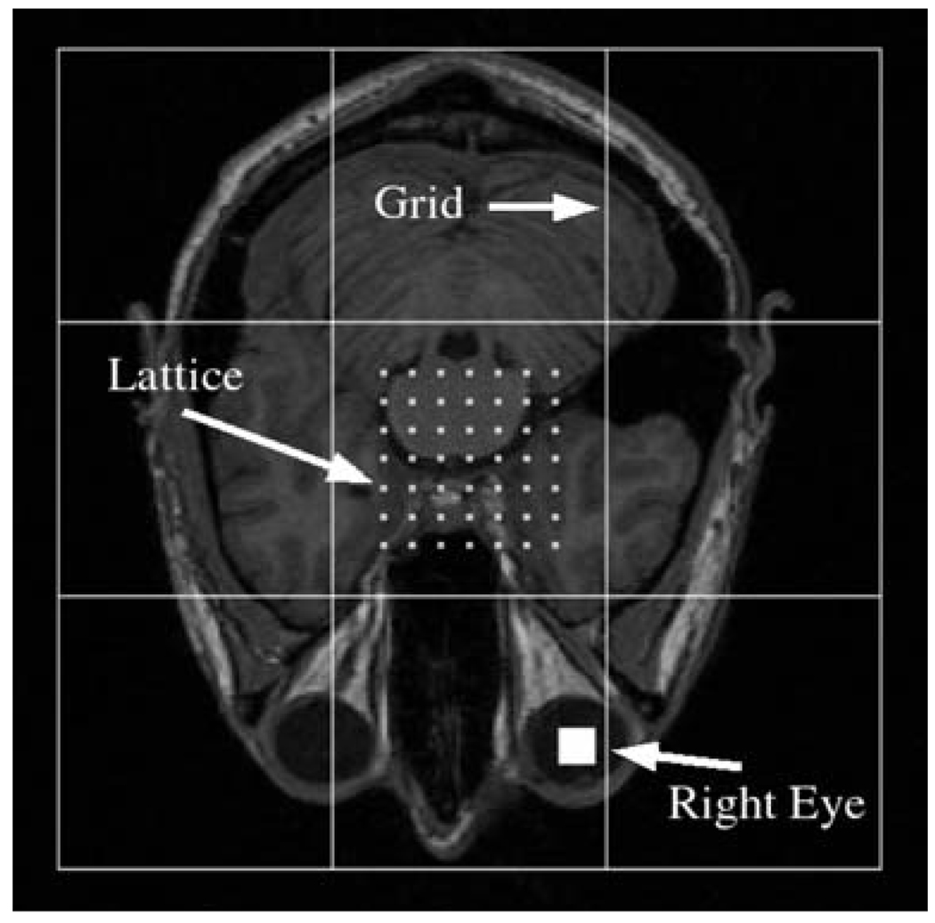
As is illustrated in Fig. 1, a lattice and grid are used to extract data from each image slice/volume in the training set. The grid contains grid cells and the intensities of all the image pixels/voxels inside each grid cell are averaged together and normalized across all the cells. Training data is extracted by placing the center of the grid at each equally-spaced lattice point and then averaging the image intensities inside the grid cells. We typically use a lattice with a 5–7 pixel/voxel spacing and have not observed better results using smaller spacings. As long as the size of each grid cell is much larger than the lattice spacing, we expect results close to those that use all the points between the lattice points.

Fig. 1.

Terminology. Training data is extracted at each lattice point by centering the grid at the point and averaging all the image intensities inside each grid cell. The solid white square at the lower-right shows the location of the center of the subject’s right eye

Although a subject’s head is normally well-centered in a brain scan, it is usually not true that the same image voxel from two different scans will correspond to the same anatomical point. However, in general the image voxels will be close to some common anatomical point. If one draws a box large enough around each image voxel, that common anatomical point will be contained by both boxes. The boxes in this case represent the initial precision; i.e., how well the anatomical point is known in both scans. The initial precision of the input point is a required input parameter for the first function in the series and is dependent upon the scale on which dissimilarities occur between images. The final precision of the output point of the last function is always limited by structural variations between subjects and noise artifacts in the image data.

Mathematical Model

We train each function in the series by defining a lattice that fills the space that represents the precision of the input to that function. For the first function, the center of the lattice is placed at the center of each image/volume, and is large enough to cover the initial precision. For the next functions in the series, the center of the lattice is placed at the user-selected anatomical point landmark (for example, the center of the subject’s right eye) and the lattice is given a size equal to the precision of the output from the previous function.

Our objective is to train the function to move every lattice point closer to the user-selected anatomical point landmark on each image/volume of the training set. The space into which the lattice points are moved represents the output precision of the function. The grid is centered at each lattice point and the image intensities inside each grid cell are computed for training. We assume that the horizontal and vertical distances from each lattice point to the anatomical point landmark are linearly correlated with the image intensities (see the Appendix) through

$$\begin{array}{lll}{I}_{11}{A}_1^k+I_{12}{A}_2^k\hfill & +\cdots +I_{1n}{A}_n^k=\hfill & D_1^k,\hfill \\ I_{21}{A}_1^k+I_{22}{A}_2^k\hfill & +\cdots +I_{2n}{A}_n^k=\hfill & D_2^k,\hfill \\ \hfill & ⋮\hfill & \hfill ⋮\hfill \\ I_{m1}{A}_1^k+I_{m2}{A}_2^k\hfill & +\cdots +I_{\mathit{\text{mn}}}{A}_n^k=\hfill & D_m^k,\hfill \end{array}$$ (1)

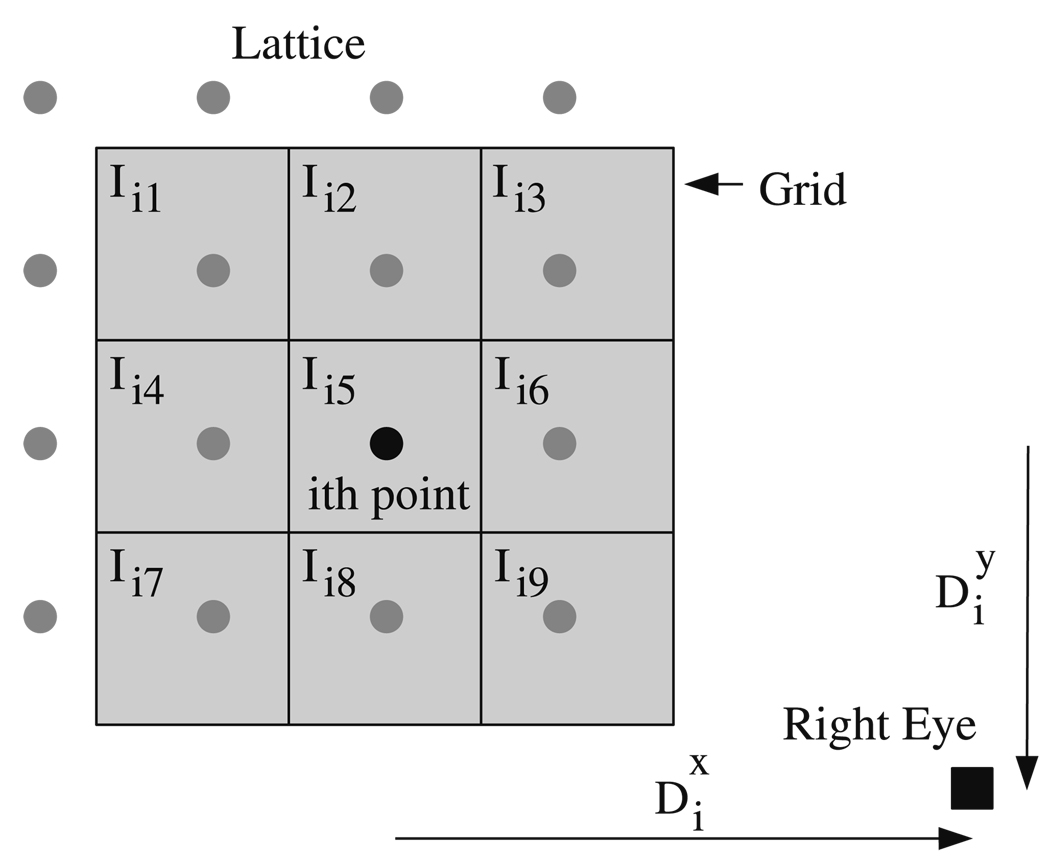
where m is the total number of lattice points in the training set, n is the number of grid cells, I_ij is the average of the image intensities in the jth grid cell at the ith lattice point, and the $A_j^k$ are unknown coefficients that are to be solved for. Each $D_i^k$ represents the distance along the kth dimension from the ith lattice point to the anatomical point landmark. In Fig. 2, there is one set of Eq. 1 for the horizontal distances $(D_i^x)$ and one set for the vertical distances $(D_i^y)$ .

Fig. 2.

Training parameters. At the ith lattice point (black circle), a grid is used to compute the average image intensity inside each grid cell (I_i1, I_i2,…I_i9). The horizontal and vertical distances from the ith lattice point to the center of the subject’s right eye (black square) are labeled $D_i^x\text{and}{D}_i^y$, respectively

Equations 1 can also be written in matrix form as

$$\mathbf{I}·{\mathbf{A}}^k={\mathbf{D}}^k,$$ (2)

where I is an m × n matrix and A^k and D^k are vectors of size n and m, respectively. Since we choose the total number of lattice points to be greater than the number of grid cells (m > n), Eq. 1 is an overdetermined set of linear equations. This being the case, we can use singular value decomposition (Press et al. 1995) to obtain a least-squares solution to Eq. 2. The singular value decomposition of the matrix I yields⁶

$$\mathbf{I}=\mathbf{U}·\mathbf{W}·{\mathbf{V}}^T,$$ (3)

where U is an m × n column-orthogonal matrix with U^T · U = 1, V is an n × n orthogonal matrix with V·V^T = 1, andWis an n × n matrix whose off-diagonal elements are zero and whose diagonal elements (the singular values w_j) are non-negative:

$$\mathbf{W}=\left(\begin{array}{llll}{w}_1\hfill & \hfill & \hfill & \hfill \\ \hfill & w_2\hfill & \hfill & \hfill \\ \hfill & \hfill & \cdots \hfill & \hfill \\ \hfill & \hfill & \hfill & w_n\hfill \end{array}\right).$$ (4)

The inverse of W is simply a matrix with the reciprocals of the singular values,

$${\mathbf{W}}^{-1}=\left(\begin{array}{llll}1/w_1\hfill & \hfill & \hfill & \hfill \\ \hfill & 1/w_2\hfill & \hfill & \hfill \\ \hfill & \hfill & \cdots \hfill & \hfill \\ \hfill & \hfill & \hfill & 1/w_n\hfill \end{array}\right),$$ (5)

for which any diagonal element may be set to zero if it is numerically ill-conditioned (Press et al. 1995). Substituting Eq. 3 into Eq. 2 and using the orthogonality relations for U and V and Eqs. 4 and 5 gives the least-squares solution for the unknown coefficients

$${\mathbf{A}}^k=\mathbf{V}·{\mathbf{W}}^{-1}·{\mathbf{U}}^T·{\mathbf{D}}^k\equiv {\mathbf{I}}^{-1}·{\mathbf{D}}^k.$$ (6)

It is only necessary to calculate the generalized inverse matrix I⁻¹ once; the same matrix is used to compute the coefficients for each dimension. Note that Eq. 6 is not an exact solution of Eq. 2 but is a solution only in the least-squares sense; I is a non-square matrix and although I⁻¹ · I = 1, in general I · I⁻¹ ≠ 1.

Two-Dimensional Results

We illustrate our approach in two-dimensions by training a sequence of functions to locate the center of each subject’s right eye in a two-dimensional image set. Each image slice in the two-dimensional set is a T1-weighted MRI image that shows the subject’s right eye. We used a training set of 64 image slices and a testing set of 32 image slices (each image slice from a different subject). The center of each subject’s right eye (the white square in the lower-right corner of Fig. 1) was manually located in each image in the training and testing sets.

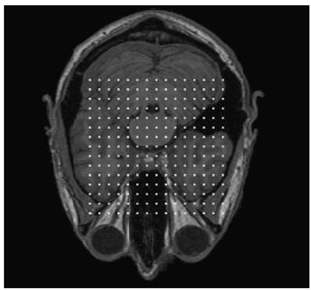
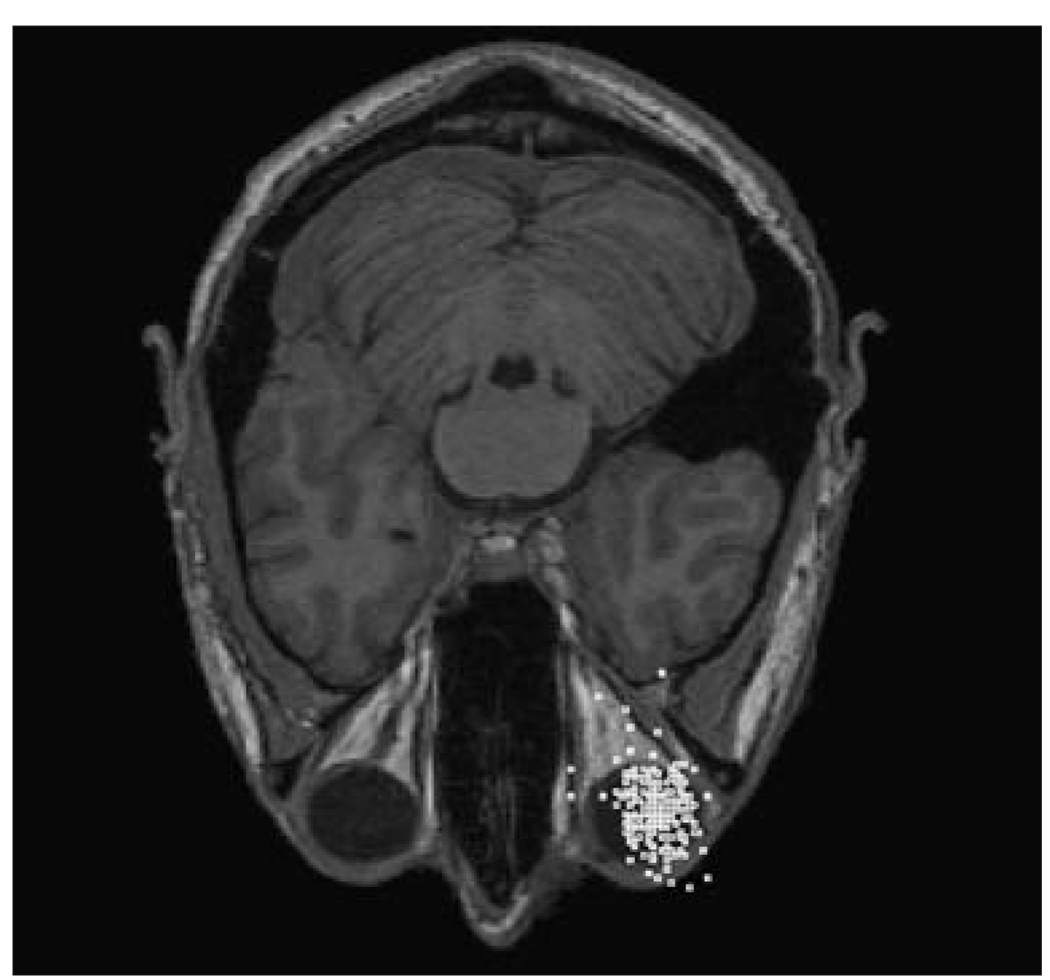
Figure 3 and Figure 4 illustrate the new locations of the lattice points on an image in the testing set when the lattice points are moved in accordance with Eqs. 1 and 6. A 5 × 5 grid of cells equal to the image size was used to compute the intensities I_ij. Most of the points in Fig. 4 fit inside a rectangle that is about one half of the lattice size. Many of the points that fall outside the rectangle were originally located near the edges of the lattice. We can determine the quality of the solution by substituting the coefficients $A_j^k$ from Eq. 6 into Eq. 1 and comparing the left-hand side of each equation with its right-hand side. We define the error at the ith lattice point for the kth dimension as

$$E_i^k\equiv A_1^k{I}_{i1}+A_2^k{I}_{i2}+\cdots +A_n^k{I}_{\mathit{\text{in}}}-D_i^k.$$ (7)

Fig. 3.

Initial locations of the lattice points. Each white square represents a lattice point and the lattice size is 38% of the image size

Fig. 4.

Final locations of the lattice points. The lattice points shown in Fig. 3 are moved in accordance with Eqs. 1 and 6. The lattice points are clustered around the subject’s right eye

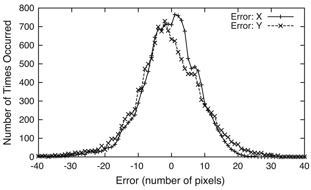
Figure 5 shows the histograms of the errors calculated at the lattice points in each dimension using Eq. 7. An error of zero in both dimensions refers to the case where a lattice point was moved exactly to the subject’s right eye. The tails of the histograms show that a small number of lattice points are not moved as close to the subject’s right eye. We note here that the shapes of the error histograms appear to be consistent with the linear least-squares assumption that the errors form a normal Gaussian distribution (Press et al. 1995). Since in our observations the error histograms are normally bell-shaped, we define the error of the solution obtained from Eq. 6 for each dimension by integrating the histogram curve area from zero in both the positive and negative directions until the sum reaches 95% of the total curve area. This 4σ-error is then the distance between the two stopping points (about four standard deviations); for example, in Fig. 5 the 4σ-error in the horizontal dimension is 32 pixels and the error in the vertical dimension is 40 pixels.

Fig. 5.

Error histograms in two-dimensions. The histograms were constructed using Eq. 7 at each lattice point. The 4σ-error (full width at four standard deviations) in the horizontal and vertical dimensions are 32 pixels and 40 pixels, respectively

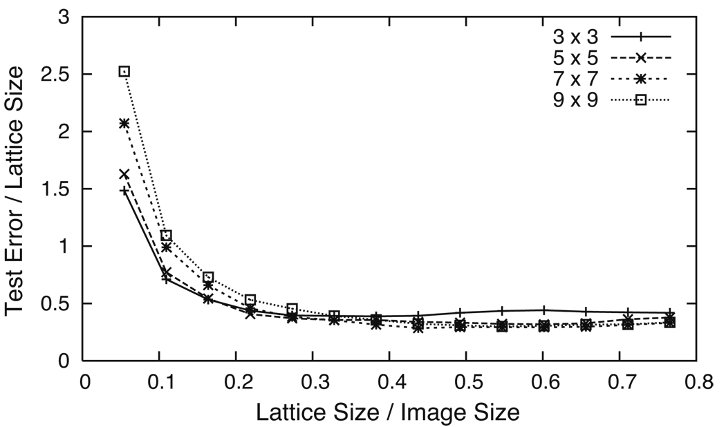
Figure 6 shows how the 4σ-errors of the testing set vary when the lattice size changes using four different grids. Each grid has a different number of grid cells (3 × 3, 5 × 5, 7 × 7, and 9 × 9) and is the same size as the image slices. The 4σ-errors from the error histograms are combined into one measurement by taking the square root of their product. It can be seen from Fig. 6 that for small lattice sizes (<10% of the image size), the test error is equal to or greater than the lattice size. In these cases, the subject’s right eye is known with a certainty less than or equal to the initial precision. But for larger lattice sizes (>20% of the image size), the test error is about half the lattice size. This is true even as the number of grid cells is increased from 9 to 81; in fact, we have noticed only slight differences when increasing the number of grid cells up to 361 (a 19 × 19 grid).

Fig. 6.

Test error versus lattice size for four equally-sized grids. Small lattice sizes (< 10% of the image size) are associated with test errors that are equal to or larger than the lattice size. Larger lattice sizes (> 20% of the image size) correspond to test errors that are about half the lattice size

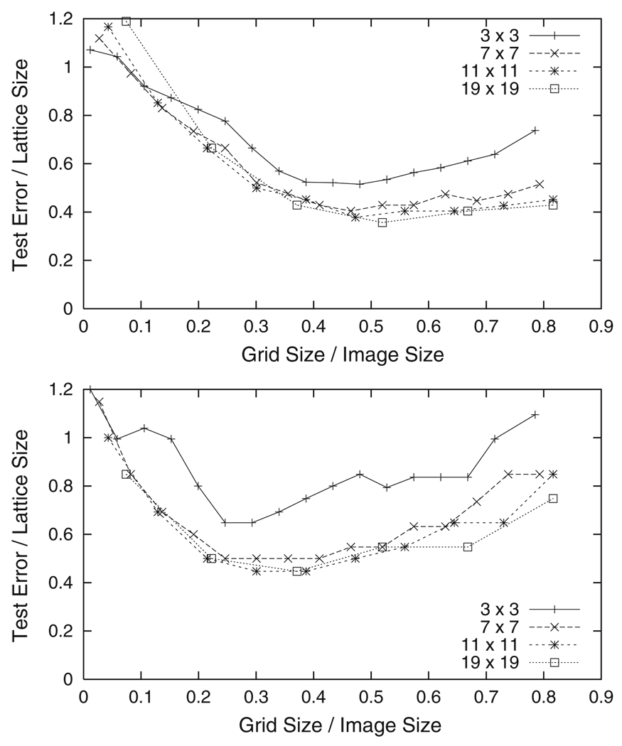
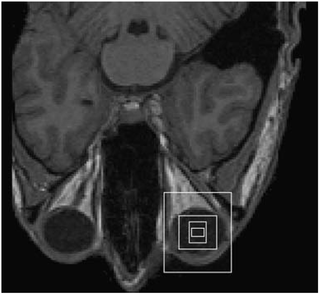
As Fig. 3 and Fig 4 illustrate, when the lattice size is large enough the lattice points of each image will be moved into a smaller area around the subject’s right eye. This area represents a new precision (how well we know where the subject’s right eye is) that is higher than the initial precision. In order to improve the precision even more, we define a new lattice of points inside the area around each subject’s right eye and repeat the above approach. The top graph in Fig. 7 shows the results when the sizes of four different grids (3 × 3, 7 × 7, 11 × 11, and 19 × 19 grid cells) are varied using the new smaller lattice (about 16% of the image size). The lowest test errors occur when the grid size is about one half the image size and the test error decreases to about one half the lattice size. The bottom graph in Fig. 7 shows the results obtained by repeating our approach once again, this time using a lattice that is 8% of the image size. Here the lowest test errors occur when the grid size is about 35% of the image size. Note that in each application of our approach as the size of the lattice decreases, the size of the grid that results in the lowest test errors gets smaller as well. Figure 8 illustrates how the precision increases as our approach is repeated. The size of the lattice at each application is represented by a white rectangle, with the largest rectangle representing the earliest iteration and the smaller rectangles representing later applications. The precision increases until the smallest rectangle is reached and no further improvement is achieved. This is because structural variations between subjects and image noise inhibit functional relationships at that resolution.

Fig. 7.

Test error versus grid size for two different lattice sizes. In the top graph the lattice size is 16% of the image size, and in the bottom graph it is 8%. As the lattice size decreases, the grid size that results in the lowest test error also decreases

Fig. 8.

Improvement in precision. Each white rectangle has dimensions equal to the 4σ-errors computed from the error histograms at each application of our approach. The precision improves after each iteration, as is illustrated by the smaller rectangles

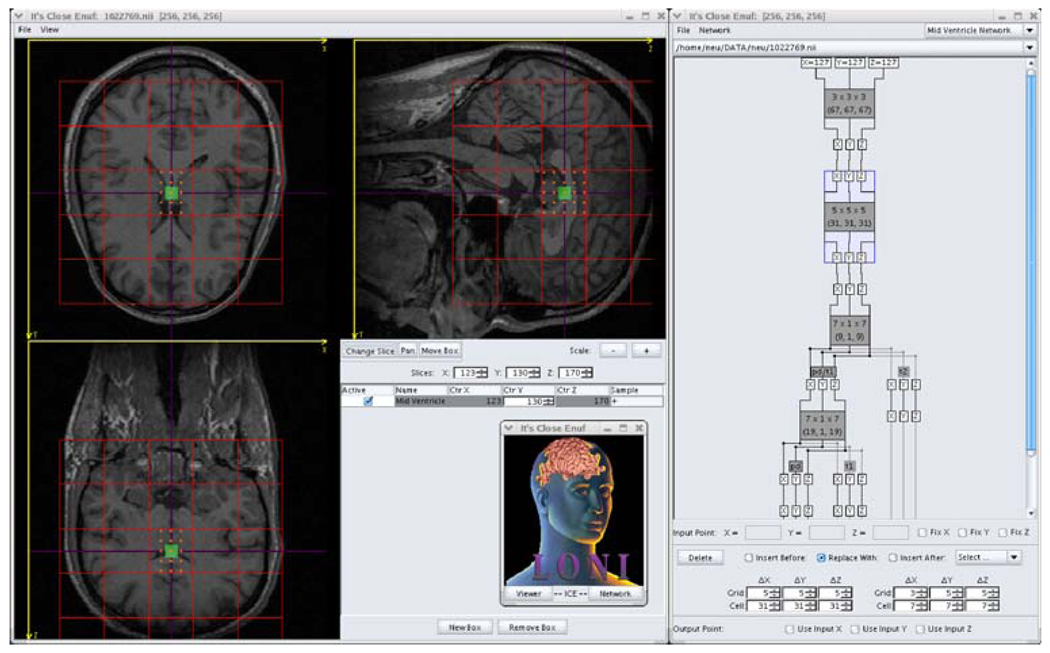
LONI ICE

LONI ICE⁷ (It’s Close Enuf) is a Java application that has been developed to assist users in training solutions using the above approach. It offers a visual interface for manually choosing training points and for changing lattice and grid parameters (Fig. 9). Each progressive application of our approach is represented as a rectangular module, and the modules are connected together to illustrate how the modules relate to one another. LONI ICE provides the means to train and test a sequence of ICE modules, and the errors at each iteration are displayed on the graphical interface. Trained modules can be saved, reloaded, and applied to new image volumes. In addition to modules that use singular value decomposition to solve Eq. 6, there are also modules that use neural networks to divide classes of images apart. Since the former modules work best when there are small structural variations between subjects, this can be useful when the training and testing sets have markedly different characteristics. We use the JAMA⁸ software package to calculate the singular value decompositions of our matrices and the JOONE⁹ software package to train the neural networks.

Fig. 9.

LONI ICE. The Java application contains a viewer for manually selecting training points and visualizing the quality of results. It also has a graphical interface for building, training, and testing modular networks

Three-Dimensional Results

We have used LONI ICE to locate the left and right eyes, nose, ventricles, central sulcus, and anterior and posterior commissures in three-dimensional MRI brain image volumes. After locating the ventricles, we also use LONI ICE to determine the MRI weighting of the image volume. The training and testing data sets for each anatomical landmark are listed in Table 2.

Table 2.

Image volumes in the training and testing sets

Anatomical landmark	Training set	Testing set
Right eye	64T1 + 64T2	16T1 + 16T2
Left eye	64T1 + 64T2	16T1 + 16T2
Bridge of nose	64T1 + 64T2	16T1 + 16T2
Ventricles	76PD + 62T1 + 72T2	20PD + 20T1 + 20T2
Anterior commissure	64T1	16T1
Posterior commissure	64T1	16T1
Lateral termination of the central sulcus	64T1	16T1

The terms “PD,” “T1,” and “T2” refer to a PD-weighted, T1-weighted, and T2-weighted MRI image volume, respectively. The number preceding each term gives the number of image volumes of that type; for example, “64T1 + 64T2” refers to 64 T1-weighted and 64 T2-weighted image volumes or 128 image volumes in the set

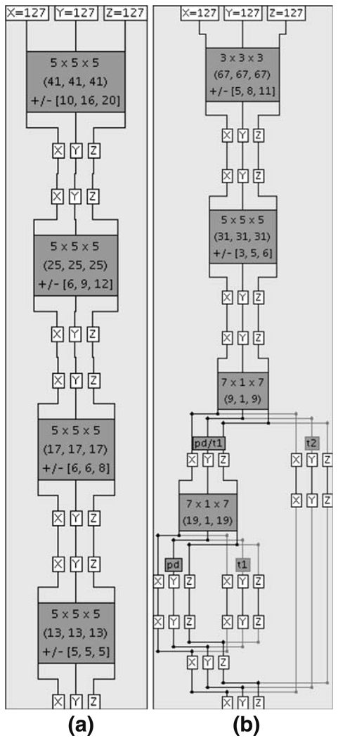
The ICE network shown in Fig. 10a is trained to locate the subject’s right eye, and the ICE network shown in Fig. 10b is trained to determine the MRI weighting (PD, T1, T2) of an image volume. We also trained two other ICE networks similar to Fig. 10a that locate the subject’s left eye and the bridge of the subject’s nose. Each gray box in Fig. 10 represents a trained ICE module and each white box displays the value of a three-dimensional coordinate (X, Y, or Z) when the ICE network is run. The input point (in both ICE networks it is the center of a 256 × 256 × 256 cube) at the top of each ICE network is processed downwards through the ICE modules and an output point is returned at the bottom. The first two rows of text on each ICE module display the grid size and grid cell size used to average voxel intensities. ICE modules that use singular value decomposition to solve Eq. 6 display the calculated precision with a third row of text, and those without a third row of text use neural networks to separate image volumes into different classes.

Fig. 10.

Two networks of LONI ICE modules. a An ICE network trained to locate the subject’s right eye. b An ICE network trained to identify the weighting (PD, T1, or T2) of an MRI image volume

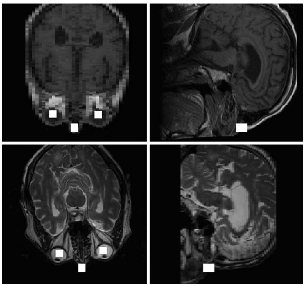
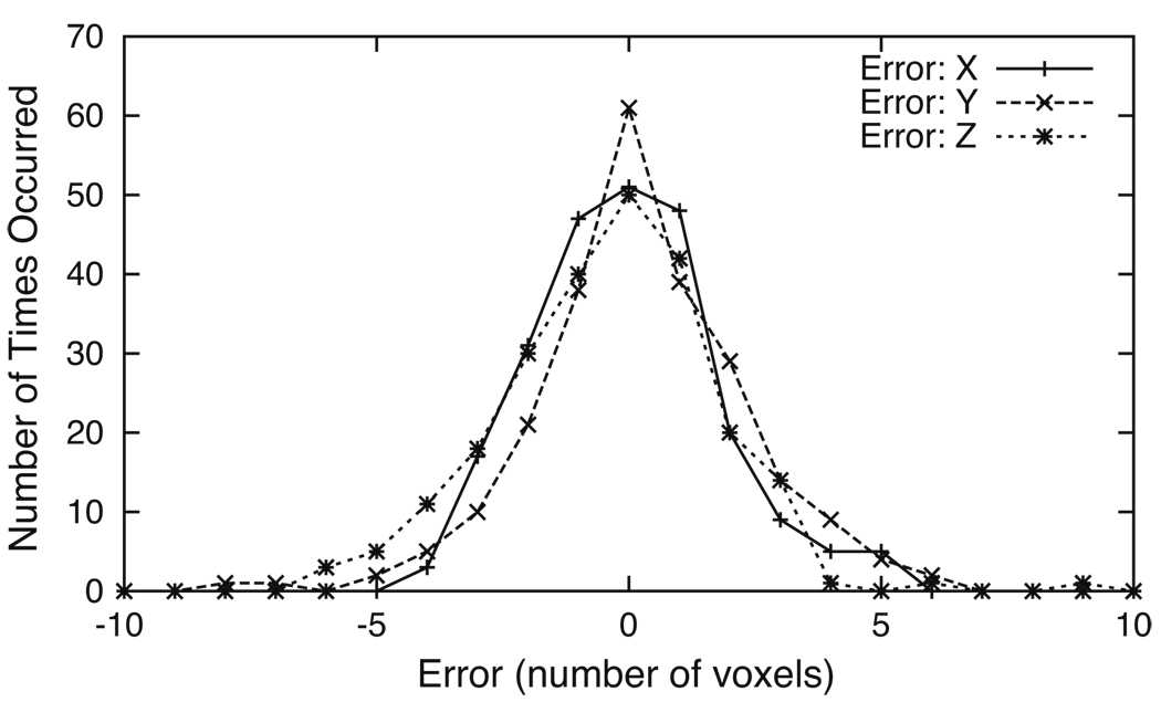
We used 64 T1-weighted and 64 T2-weighted image volumes to train the eyes and nose ICE networks and 16 T1-weighted and 16 T2-weighted image volumes for testing. The results for a T1-weighted (top) and a T2-weighted (bottom) image volume from the testing set are illustrated in Fig. 11. The solid white squares graphically depict how precisely the bridge of the nose and the right and left eyes are determined. Each eye is detected within a rectangular volume of (10, 10, 10) voxels and each nose bridge is located within a rectangular volume of (10, 12, 16) voxels. Even though the image volumes have different resolutions and the subject’s nose is cut off in the T1-weighted image volume, the anatomical point landmarks are still well-determined. In order to verify the accuracy of the right eye ICE network, we computed a histogram of the errors determined from 144 T1-weighted and 92 T2-weighted image volumes. The errors are defined as the differences in each dimension between the manually selected points and the points output by the ICE network. As Fig. 12 illustrates, the output points are correctly localized to the error bounds [(−5, 5) in each dimension] computed by our approach.

Fig. 11.

Automatic detection of the eyes and bridge of the nose in a T1-weighted (top) and a T2-weighted (bottom) image volume. The axial and sagittal view planes intersect the bridge of the subject’s nose. The solid white squares show how precisely the anatomical point landmarks are determined

Fig. 12.

Error histograms for the right eye ICE network. The errors in all three dimensions are localized within the calculated error bounds of (−5, 5) voxels

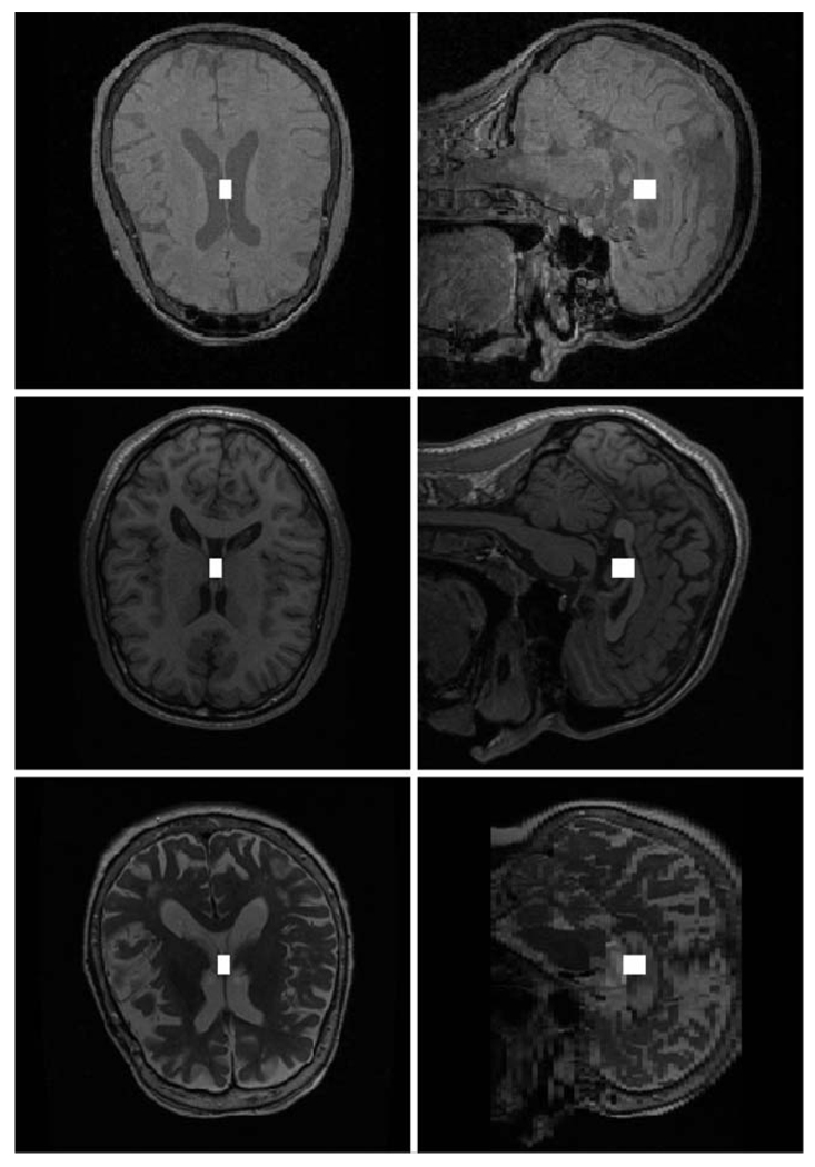
As Fig. 10b illustrates, our strategy for determining MRI weighting starts with two ICE modules that locate the center of the subject’s ventricles, and are followed by an ICE module that classifies the image volume as either PD-/T1-weighted or T2-weighted. When the image volume is classified as PD-/T1-weighted, an additional ICE module is used to further classify it as PD-weighted or T1-weighted. We use the subject’s ventricles for classification because the intensities of the voxels in that region are different for the three MRI weighting types. The MRI weighting ICE network was trained using 76 PD-weighted, 62 T1-weighted, and 72 T2-weighted image volumes and was tested using 20 PD-weighted, 20 T1-weighted, and 20 T2-weighted image volumes. Figure 13 shows the results for a PD-weighted (top), T1-weighted (middle), and T2-weighted (bottom) image volume from the testing set. The solid white squares show the center of each subject’s ventricles as output by the second ICE module in Fig. 10b. All the image volumes from the training and testing sets were correctly classified.

Fig. 13.

Automatic detection of the ventricles in a PD-weighted (top), T1-weighted (middle), and T2-weighted (bottom) image volume. Both the axial and sagittal views for each image volume are shown. The solid white squares show how precisely the center of the ventricles are determined

Table 3 summarizes how well the trained LONI ICE networks can locate anatomical landmarks in MRI image volumes of adult heads. Included in this table are results for the anterior and posterior commissures. Only T1-weighted images were used for training and testing because of the difficulty in manually finding the commissures in T2-weighted images. There are also results for the lateral termination of the central sulcus (defined as the extrapolated intersection of the central sulcus with the Sylvian fissure on the surface of the right hemisphere). The central sulcus point was determined by manually removing the skull in each image volume and then generating a brain surface. Each point was chosen by viewing and manipulating each surface in a three-dimensional display.

Table 3.

Precisions of trained LONI ICE networks that locate anatomical landmarks in MRI images of adult heads

Anatomical landmark	Precision (X) (mm)	Precision (Y) (mm)	Precision (Z) (mm)
Right eye	±5	±5	±5
Left eye	±5	±5	±5
Bridge of nose	±5	±6	±8
Ventricles	±3	±5	±6
Anterior commissure	±3	±5	±6
Posterior commissure	±3	±5	±5
Lateral termination of the central sulcus	±6	±8	±6

The networks were trained using the training and testing sets in Table 2.

Discussion

Applications

The LONI ICE networks that locate a subject’s eyes and nose bridge are pertinent to the removal of facial features from MRI brain images. We anticipate that by blacking-out image voxels around the output points of the ICE networks, one can develop a relatively quick and accurate application that performs facial deidentification. Since the ICE networks can locate facial features in T1-weighted and T2-weighted images, it will be applicable for both types of images, unlike current approaches (Shattuck et al. 2003; Bischoff-Grethe et al. 2004). The LONI ICE network that determines the MRI weighting of an image volume has a practical value because in our experience there does not exist a formula that can reliably return the MRI weighting from common scanner acquisition parameters (i.e., echo time, repetition time, etc.) alone. Further, it is often the case that the file format (e.g., ANALYZE¹⁰ or MINC¹¹) used to store image voxels does not contain information about the MRI weighting or the acquisition parameters of the scan. An automatic method for determining the MRI weighting is particularly useful when, for example, archiving a large set of image files and populating a database that can be queried over MRI weighting type. We have noticed that this ICE network does sometimes misclassify T1-weighted image volumes as PD-weighted image volumes when the subject’s ventricles are very small. Although the center of the ventricles are located properly, the neural network that is trained to classify the images as PD-weighted or T1-weighted can give incorrect results. But we have consistently found that when we add these problematic images to the training set and retrain the ICE network, it correctly classifies these images.

Structural variations between subjects primarily determine the precisions of the LONI ICE modules that use singular value decomposition to solve Eq. 6. For example, in Table 3 the lateral termination of the subject’s right central sulcus is known with less precision than the subject’s right eye because cortical landmarks are more variable in location than eye landmarks. Also, in Fig. 11 the bridge of the subject’s nose is known with less certainty sagittally (16 voxels) than the subject’s eyes (10 voxels). This is because the eyes normally appear as predictable ellipsoids across subjects whereas the region around the nose tends to have higher variance. In contrast, the ICE modules that use neural networks yield the best results when the differences between subjects can be separated into distinct classes. Variations in intensity (e.g., between T1-weighted and T2-weighted images) are less important than structural variations because one can find least-squares coefficients that provide a good fit to different intensity correlations. Since we spatially average voxel intensities using grids, our approach will produce the best results when structural variations are smaller than the sizes of the grid cells.

Computational Considerations

The training process used by LONI ICE is divided into two main computational steps. The first step calculates the average voxel intensities at each lattice point in the training set, and the second step uses the results of the first step to construct the matrices in Eq. 2 and performs the singular value decompositions. Using an image volume with dimensions 205 × 240 × 240, completion of the first step requires about 8 min on a computer with a 3.2 GHz CPU and 2G of RAM. Since each image volume in the training set can be processed separately, we usually perform the computations in parallel on our grid computing architecture. The singular value decomposition calculations needed for the four module ICE network shown in Fig. 10a take about 10 min to finish using a training set of 128 image volumes. Although the singular value decompositions can be performed in parallel as well, the current version of the LONI ICE application performs them serially. Executing a trained ICE network requires about 6 s to read in and reformat the image volume and about 2 s to run the actual ICE network.

Although our approach can be applied to any number of dimensions, memory limitations practically impede the singular value decomposition computations for higher dimensions, which are performed entirely in computer memory. This is because the size of the intensity matrix I grows geometrically with the number of dimensions; for example, in two-dimensions a 9 × 9 grid has m = 81 elements but in three-dimensions a 9 × 9 × 9 grid jumps to m = 729 elements (effectively increasing the size of I by an order of magnitude). Fortunately, as is illustrated in Fig. 7, we have empirically found that grids with a low number of cells (e.g., 7 × 7) yield test errors comparable to grids with a high number of cells (e.g., 19 × 19). In practice, we rarely need to use grids with more than 5 × 5 × 5 cells in three-dimensions.

It should be noted that the output point of a trained LONI ICE module is not guaranteed to lie within the error ranges shown on the module. As Fig. 5 illustrates, there are tails to the error histograms that indicate there is a small chance that the output point will fall outside the error bounds. We have found that these points typically originate near, but are not entirely constrained to, the edges of the lattice. Increasing the size of the lattice will help reduce the possibility of an errant output point, but it will also decrease the trained module’s precision, which may then require the addition of more ICE modules to a network.

Comparison with Linear Registration

We have compared a standard linear registration technique with our method and have found the accuracies of both approaches to be the same. The linear registration technique deduces anatomical point landmarks by transforming an image volume into an “atlas” space. We created such an atlas using the Automated Image Registration (AIR) package (Woods et al. 1998) and a set of 64 resampled T1-weighted image volumes. The first image volume was chosen to be the target, and affine transforms were computed to best map each image volume into the target space. These transforms were combined into an “averaged” transform, and a preliminary atlas was created by combining all the image volumes in the averaged space. After computing a second set of affine transforms that mapped each image volume into the preliminary atlas space, the final atlas was created by combining the image volumes in the preliminary atlas space. An anatomical point landmark was found by locating the point landmark on the atlas, computing the affine transform that maps an image volume to the atlas, and then transforming the point landmark from the atlas to the image volume.

Although the accuracies of both approaches are the same, we have found that it typically takes minutes to compute the affine transform to the atlas space whereas our method requires only several seconds of CPU time. This makes our method preferrable when only a few anatomical point landmarks are desired in a relatively short amount of time.

Information Sharing Statement

Data used in the preparation of this paper were obtained from the Alzheimer’s Disease Neuroimaging Initiative (ADNI) database.¹² The ADNI was launched in 2003 by the National Institute on Aging (NIA), the National Institute of Biomedical Imaging and Bioengineering (NIBIB), the Food and Drug Administration (FDA), private pharmaceutical companies and non-profit organizations, as a $60 million, 5-year public-private partnership. The primary goal of ADNI has been to test whether serial magnetic resonance imaging (MRI), positron emission tomography (PET), other biological markers, and clinical and neuropsychological assessment can be combined to measure the progression of mild cognitive impairment (MCI) and early Alzheimer’s disease (AD). Determination of sensitive and specific markers of very early AD progression is intended to aid researchers and clinicians to develop new treatments and monitor their effectiveness, as well as lessen the time and cost of clinical trials.

LONI ICE is freely available (http://www.loni.ucla.edu/Software) under the UCLA Laboratory of Neuro Imaging’s terms and conditions of use license.

Appendix: Relation to Cross-Correlation

Cross-correlation (Russ 2006) is a well-known method in image processing that is commonly used to find features within images. The shift required to align a target image with another image is determined by sliding the target image along the latter image and summing the products of all overlaid pixel values at each location. The sum is a maximum where the images are best matched.

In this Appendix we relate cross-correlation to the method described in this paper in one-dimension; it is straight-forward to extend this relation to two and three dimensions. If I is a one-dimensional image intensity function and is displaced a distance x relative to another function A, the cross-correlation is defined as

$${\displaystyle \int A(g)I(g+x)\mathit{\text{dg}}.}$$ (8)

In the limit of small x, we approximate I(g + x) as I(g) + xI′ (g) and note that Eq. 8 has the form

$${\displaystyle \int A(g)[I(g)+xI\prime (g)]\mathit{\text{dg}}~D+\mathit{\text{xC}},}$$ (9)

where D and C are constants. In particular, if we choose C = −1, then in this limit the integral is equal to the distance between I and A (with D defined as the distance between them at x = 0).

In our case, we are choosing a function for the cross-correlation integral and solving for A (as opposed to being given I and A and computing the integral). We are then interested in finding a function A that makes

$${\displaystyle \int A(g)I(g+x)\mathit{\text{dg}}=D-x}$$ (10)

approximately true. The integral can be approximated by evaluating the integrand at n locations that are a distance δ apart

$${\displaystyle \sum _{j=1}^{n}A(j\delta )I(j\delta +x)=D-x,}$$ (11)

and if the range of x is evaluated in m steps of length Δ, we have the system of equations given in Eq. 1 where A_j = A(jδ), I_ij = I(jδ + iΔ), and D_i = D − iΔ. The coefficients A_j are determined using least-squares to minimize the differences between both sides of Eq. 10.

One advantage of using least-squares is that the solution is insensitive to constant changes in intensity. For example, let I₁(x) and I₂(x) be image intensities where I₂(x) = I₁(x) + I₀ and I₀ is a constant. Then the function A that minimizes the differences between both sides of the equations

$$\begin{array}{l}{\displaystyle \int A(g)I_1(g+x)\mathit{\text{dg}}=D-x,}\hfill \\ {\displaystyle \int A(g)I_2(g+x)\mathit{\text{dg}}=D-x,}\hfill \end{array}$$ (12)

is also the function that minimizes the differences between both sides of the equations

$${\displaystyle \int A(g)I_1(g+x)\mathit{\text{dg}}=D-x,}$$ (13)

$${\displaystyle \int A(g)I_0\mathit{\text{dg}}=0,}$$ (14)

by subtracting the two equations. Equation 14 states that the contributions of constant intensity terms are minimized.

References

- Alker M, Frantz S, et al. Improving the robustness in extracting 3D point landmarks based on deformable models. Proceedings of the 23rd DAGM-Symposium on pattern recognition; 2001. pp. 108–115. [Google Scholar]
- Arun KS, Huang TS, et al. Least square fitting of two 3D point sets. IEEE Transactions on Pattern Analysis and Machine Intelligence. 1987;1987(9):698–700. doi: 10.1109/tpami.1987.4767965. [DOI] [PubMed] [Google Scholar]
- Barrett WA, Mortensen EN. Interactive live-wire boundary extraction. Medical Image Analysis. 1997;1(4):331–341. doi: 10.1016/s1361-8415(97)85005-0. [DOI] [PubMed] [Google Scholar]
- Besl PJ, McKay ND. A method for registration of 3-D shapes. IEEE Transactions on Pattern Analysis and Machine Intelligence. 1992;14(2):239–256. [Google Scholar]
- Boykov Y, Jolly M. Interactive graph cuts for optimal boundary and region segmentation of objects in N–D images; International Conference on Computer Vision; 2001. pp. 105–112. [Google Scholar]
- Bischoff-Grethe A, Fischl B, et al. A technique for the deidentification of structural brain MR images. Budapest, Hungary: Human Brain Mapping; 2004. [DOI] [PMC free article] [PubMed] [Google Scholar]
- Chandra DVS. Digital image watermarking using singular value decomposition. Proc. 45th IEEE Midwest symp. on circuits and systems; 2002. pp. 264–267. [Google Scholar]
- Chen PC, Pavlidis T. Segmentation by textures using correlation. IEEE Transactions on Pattern Analysis and Machine Intelligence. 1983;5(1):64–69. doi: 10.1109/tpami.1983.4767346. [DOI] [PubMed] [Google Scholar]
- Cox IJ, Rao SB, et al. Ratio regions: A technique for image segmentation; Proc. International Conference on Pattern Recognition; 1996. pp. 557–564. [Google Scholar]
- Daneels D, Van Campenhout D, et al. Interactive Outlining: An improved approach using active contours. SPIE Proceedings of Storage and Retrieval for Image and Video Databases. 1993;1908:226–233. [Google Scholar]
- Davis LS, Johns SA, et al. Texture analysis using generalized cooccurrence matrices. IEEE Transactions on Pattern Analysis and Machine Intelligence. 1979;1:251–259. doi: 10.1109/tpami.1979.4766921. [DOI] [PubMed] [Google Scholar]
- Ende G, Treuer H, et al. Optimization and evaluation of landmark-based image correlation. Physics in Medicine & Biology. 1992;37(1):261–271. doi: 10.1088/0031-9155/37/1/019. [DOI] [PubMed] [Google Scholar]
- Falco AX, Udupa JK, et al. User-steered image segmentation paradigms: Live wire and live lane. Graphical Models and Image Processing. 1998;60(4):233–260. [Google Scholar]
- Fang S, Raghavan R, et al. Volume morphing methods for landmark based 3D image deformation; SPIE International Symposium on Medical Imaging; 1996. pp. 404–415. [Google Scholar]
- Fischl B, Salat DH, et al. Whole brain segmentation: Automated labeling of neuroanatomical structures in the human brain. Neuron. 2002;33(3):341–355. doi: 10.1016/s0896-6273(02)00569-x. [DOI] [PubMed] [Google Scholar]
- Fitzpatrick JM, Reinhardt JM. Automatic land-marking of magnetic resonance brain images. Proceedings SPIE. 2005;1329:1329–1340. [Google Scholar]
- Frantz S, Rohr K, et al. Localization of 3d anatomical point landmarks in 3d tomographic images using deformable models. Proceedings on MICCAI. 2000;2000:492–501. [Google Scholar]
- Gorodetski VI, Popyack LJ, et al. SVD-based approach to transparent embedding data into digital images. Proceedings on International Workshop on Mathematical Methods, Models and Architectures for Computer Network Security. 2001;2052:263–274. [Google Scholar]
- Han Y, Park H. Automatic registration of brain magnetic resonance images based on talairach reference system. Journal of Magnetic Resonance Imaging. 2004;20(4):572–580. doi: 10.1002/jmri.20168. [DOI] [PubMed] [Google Scholar]
- Hansen PC, Jensen SH. FIR filter representation of reduced-rank noise reduction. IEEE Transactions on Signal Proceedings. 1998;46(6):1737–1741. [Google Scholar]
- Hartkens T, Rohr K, et al. Evaluation of 3D operators for the detection of anatomical point landmarks in MR and CT Images. Computer Vision and Image Understanding. 2002;86(2):118–136. [Google Scholar]
- Hill DL, Hawkes DJ, et al. Registration of MR and CT images for skull base surgery using point-like anatomical features. British Journal of Radiology. 1991;64(767):1030–1035. doi: 10.1259/0007-1285-64-767-1030. [DOI] [PubMed] [Google Scholar]
- Huang T, Narendra P. Image restoration by singular value decomposition. Applied Optics. 1974;14(9):2213–2216. doi: 10.1364/AO.14.002213. [DOI] [PubMed] [Google Scholar]
- Kalman D. A singularly valuable decomposition: The SVD of a matrix. The College Mathematics Journal. 1996;27(1):2–23. [Google Scholar]
- Kass M, Witkin A, et al. Snakes: Active contour models. International Journal of Computer Vision. 1987;1(4):321–331. [Google Scholar]
- Konstantinides K, Yovanof GS. Application of SVD-based spatial filtering to video sequences; IEEE International Conference on Acoustics; 1995. pp. 2193–2196. [Google Scholar]
- Konstantinides K, Natarajan B, et al. Noise estimation and filtering using block-based singular value decomposition. IEEE Transactions on Image Process. 1997;6(3):479–483. doi: 10.1109/83.557359. [DOI] [PubMed] [Google Scholar]
- Le Briquer L, Lachmann F, et al. Using local extremum curvatures to extract anatomical landmarks from medical images. Proceedings on SPIE. 1993;1898:549–558. [Google Scholar]
- MacDonald D, Avis D, Evan AC. Multiple surface identification and matching in magnetic resonance imaging. Proceedings of the Society of Photo-optical Instrumentation Engineers. 1994;2359:160–169. [Google Scholar]
- McInerney T, Dehmeshki H. User-defined b-spline template-snakes. Medical Image Computing and Computer-Assisted Intervention. 2003;2879:746–753. [Google Scholar]
- Meyer F, Beucher S. Morphological segmentation. Journal of Visual Communications and Image Representation. 1990;1(1):21–46. [Google Scholar]
- Mortensen EN, Barrett WA. Intelligent scissors for image composition. Proceedings of the ACM SIGGRAPH ‘95: Computer graphics and interactive techniques. 1995;Vol. 191–198 [Google Scholar]
- O’Leary DP, Peleg S. Digital image compression by outer product expansion. IEEE Transactions on Communications. 1983;31(3):441–444. [Google Scholar]
- Pennec X, Ayache N, et al. Handbook of medical imaging. 1st edn. San Diego, CA: Academic; 2000. Landmark-based registration using features identified through differential geometry. [Google Scholar]
- Peters TM, Davey BLK, et al. Three-dimensional multi-modal image-guidance for neurosurgery. IEEE Transactions on Medical Imaging. 1996;15(2):121–128. doi: 10.1109/42.491414. [DOI] [PubMed] [Google Scholar]
- Pohl KM, Wells WM, et al. Incorporating non-rigid registration into expectation maximization algorithm to segment MR Images. Fifth international conference on medical image computing and computer assisted intervention; Tokyo, Japan. 2002. [DOI] [PMC free article] [PubMed] [Google Scholar]
- Press WH, Teukolsky SA, Vetterling WT, Flannery BP. Numerical recipies in C: The art of scientific computing. 2nd edn. Cambridge, UK: Cambridge University Press; 1995. [Google Scholar]
- Rohr K. On 3d differential operators for detecting point landmarks. Image and Vision Computing. 1997;15(3):219–233. [Google Scholar]
- Rohr K. Landmark-based image analysis using geometric and intensity models. 1st edn. Dordrecht, The Netherlands: Kluwer; 2001. [Google Scholar]
- Russ JC. The image processing handbook. 5th edn. Boca Raton, FL: CRC Press; 2006. [Google Scholar]
- Sethian JA. Level set methods and fast marching methods. 2nd edn. Cambridge, UK: Cambridge University Press; 1999. [Google Scholar]
- Shattuck DW, Rex DE, et al. JohnDoe: Anonymizing MRI data for the protection of research subject confidentiality. 9th annual meeting of the organization for human brain mapping; New York, New York. 2003. [Google Scholar]
- Sirovich L, Kirby M. Low dimensional procedure for the characterization of human faces. Journal of the Optical Society of America A. 1987;4(3):519–524. doi: 10.1364/josaa.4.000519. [DOI] [PubMed] [Google Scholar]
- Strasters KC, Little JA, et al. Anatomic landmark image registration: Validation and comparison. CVR Med/MRCAS. 1997;1997:161–170. [Google Scholar]
- Thirion J. Extremal points: Definition and application to 3D image registration; Proceedings of the Conference on Computer Vision and Pattern Recognition; 1994. pp. 587–592. [Google Scholar]
- Toga AW. Brain warping. 1st edn. San Diego, CA: Academic; 1999. [Google Scholar]
- Turk MA, Pentland AP. Eigenfaces for recognition. Journal of Cognitive Neuroscience. 1991;3(1):71–86. doi: 10.1162/jocn.1991.3.1.71. [DOI] [PubMed] [Google Scholar]
- Woods RP, Grafton ST, et al. Automated image registration: I. General methods and intrasubject, intramodality validation. Journal of Computer Assisted Tomography. 1998;22(1):139–152. doi: 10.1097/00004728-199801000-00027. [DOI] [PubMed] [Google Scholar]
- Wörz S, Rohr K, et al. 3D parametric intensity models for the localization of different types of 3D anatomical point landmarks in tomographic images; DAGM-Symposium; 2003. pp. 220–227. [Google Scholar]
- Yushkevich PA, Piven J, et al. User-guided 3D active contour segmentation of anatomical structures: Significantly improved efficiency and reliability. Neuroimage. 2006;31(3):1116–1128. doi: 10.1016/j.neuroimage.2006.01.015. [DOI] [PubMed] [Google Scholar]