Excited-State Electronic Structure with Configuration Interaction Singles and Tamm–Dancoff Time-Dependent Density Functional Theory on Graphical Processing Units

Abstract

Excited-state calculations are implemented in a development version of the GPU-based TeraChem software package using the configuration interaction singles (CIS) and adiabatic linear response Tamm–Dancoff time-dependent density functional theory (TDA-TDDFT) methods. The speedup of the CIS and TDDFT methods using GPU-based electron repulsion integrals and density functional quadrature integration allows full ab initio excited-state calculations on molecules of unprecedented size. CIS/6-31G and TD-BLYP/6-31G benchmark timings are presented for a range of systems, including four generations of oligothiophene dendrimers, photoactive yellow protein (PYP), and the PYP chromophore solvated with 900 quantum mechanical water molecules. The effects of double and single precision integration are discussed, and mixed precision GPU integration is shown to give extremely good numerical accuracy for both CIS and TDDFT excitation energies (excitation energies within 0.0005 eV of extended double precision CPU results).

Introduction

Single excitation configuration interaction (CIS),(1) time-dependent Hartree–Fock (TDHF), and linear response time-dependent density functional theory (TDDFT)²⁻⁶ are widely used for ab initio calculations of electronic excited states of large molecules (more than 50 atoms, thousands of basis functions) because these single-reference methods are computationally efficient and straightforward to apply.⁷⁻⁹ Although highly correlated and/or multireference methods, such as multireference configuration interaction (MRCI),(10) multireference perturbation theory (MRMP(11) and CASPT2), (12)and equation-of-motion coupled cluster methods (SAC-CI(13) and EOM-CC),^14,15 allow for more reliably accurate treatment of excited states, including those with double excitation character, these are generally too computationally demanding for large molecules.

CIS/TDHF is essentially the excited-state corollary of the ground-state Hartree–Fock (HF) method and thus similarly suffers from a lack of electron correlation. Because of this, CIS/TDHF excitation energies are consistently overestimated, often by ∼1 eV.(8) The TDDFT method includes dynamic correlation through the exchange–correlation functional, but standard nonhybrid TDDFT exchange–correlation functionals generally underestimate excitation energies, particularly for Rydberg and charge-transfer states.(5) The problem in charge-transfer excitation energies is due to the lack of the correct 1/r Coulombic attraction between the separated charges of the excited electron and hole.(16) Charge-transfer excitation energies are generally improved with hybrid functionals and also with range separated functionals that separate the exchange portion of the DFT functional into long- and short-range contributions.¹⁷⁻²¹ Neither CIS nor TDDFT (with present-day functionals) properly includes the effects of dispersion but promising results have been obtained with an empirical correction to standard DFT functionals,^22,23 and there are continued efforts to include dispersion directly in the exchange–correlation functional.^24,25 Both the CIS and TDDFT(26) single reference methods lack double excitations and are unable to model conical intersections or excitations in molecules that have multireference character.^27,28 In spite of these limitations, the CIS and TDDFT methods can be generally expected to reproduce trends for one-electron valence excitations, which are a majority of the transitions of photochemical interest. TDDFT using hybrid density functionals, which include some percentage of HF exact exchange, has been particularly successful in modeling the optical absorption of large molecules. Furthermore, the development of new DFT functionals and methods is an avid area of research, with many new functionals introduced each year. Thus it is a virtual certainty that the quality of the results available from TDDFT will continue to increase. A summary of the accuracy currently available for vertical excitation energies is available in a recent study by Jacquemin et al. which compares TDDFT results using 29 functionals for ∼500 molecules.(29)

Although CIS and TDDFT are the most tractable methods for excited states of large molecules, their computational cost still prevents application to many systems of photochemical interest. Thus, there is considerable interest in extending the capabilities of CIS/TDDFT to even larger molecules, beyond hundreds of atoms.

Quantum mechanics/molecular mechanics (QM/MM) schemes provide a way to model the environment of a photophysically interesting molecule by treating the molecule with QM and the surrounding environment with MM force fields.³⁰⁻³⁴ However, it is difficult to know when the MM approximations break down and when a fully QM approach is necessary. With fast, large-scale CIS/TDDFT calculations, all residues of a photoactive protein could be treated quantum mechanically to explore the origin of spectral tuning, for example. Explicit effects of solvent–chromophore interactions, including hydrogen bonding, charge transfer, and polarization, could be fully included at the ab initio level in order to model solvatochromic shifts.

One potential route to large scale CIS and TDDFT calculations is through exploitation of the stream processing architectures(35) now widely available in the form of graphical processing units (GPUs). The introduction of the compute unified device architecture(36) (CUDA) as an extension to the C language has greatly simplified GPU programming, making it more easily accessible for scientific programming. GPUs have already been applied to achieve speed-ups of orders of magnitude in ground-state electronic structure,³⁷⁻⁴⁰ ab initio molecular dynamics(41) and empirical force field-based molecular dynamics calculations.⁴²⁻⁴⁵

In this article we extend our implementation of GPU quantum chemistry in the newly developed TeraChem program(46) beyond our previous two-electron integral evaluation(47) and ground-state self-consistent field,^39,48,49 geometry optimization, and dynamics calculations(41) to also include the calculation of excited electronic states. We use GPUs to accelerate both the matrix multiplications within the CIS/TDDFT procedure and also the integral evaluation (these steps comprise most of the effort in the calculation). The computational efficiency that arises from the use of redesigned quantum chemistry algorithms on GPU hardware to evaluate electron repulsion integrals (ERIs) allows full QM treatment of the excited states of very large systems—both large chromophores and chromophores in which the environment plays a critical role and should be treated with QM. We herein present the results of implementing CIS and TDDFT within the Tamm–Dancoff approximation using GPUs to drastically speed up the bottleneck two-electron integral evaluation, density functional quadrature, and matrix multiplication steps. This results in CIS calculations over 400 times faster than those achieved running on a comparable CPU platform. Benchmark CIS/TDDFT timings are presented for a variety of systems.

CIS/TDDFT Implementation using GPUs

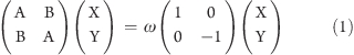
The linear response formalism of TDHF and TDDFT has been thoroughly presented in review articles.^4,7,8,50 Only the equations relevant for this work are presented here, and real orbitals are assumed throughout. The TDHF/TDDFT working equation for determining the excitation energies ω and corresponding X and Y transition amplitudes is

where for TDHF (neglecting spin indices for simplicity):

and for TDDFT:

The two electron integrals (ERIs) are defined as

and within the adiabatic approximation of density functional theory, in which the explicit time dependence of the exchange–correlation functional is neglected:

The i,j and a,b indices represent occupied and virtual molecular orbitals (MOs), respectively, in the HF/Kohn–Sham (KS) ground-state determinant.

Setting the B matrix to zero within TDHF results in the CIS equation, while in TDDFT this same neglect yields the equation known as the Tamm–Dancoff approximation (TDA):

In part because DFT virtual orbitals provide a better starting approximation to the excited state than HF orbitals, the TDA generally gives results that are very close to the full linear response TDDFT results for nonhybrid DFT functionals at equilibrium geometries.^7,8,51 Furthermore, previous work has shown that a large contribution from the B matrix in TDDFT (and to a lesser extent also in TDHF) is often indicative of a poor description of the ground state, either due to singlet–triplet instabilities or multireference character.(52) Casida and co-workers have examined the breakdown of TDDFT in modeling photochemical pathways(52) and have come to the conclusion that “the TDA gives better results than does conventional TDDFT when it comes to excited-state potential energy surfaces in situations where bond breaking occurs.” Thus, if there is substantial deviation between the full TDDFT and TDA-TDDFT excitation energies, then the TDA results will often be more accurate.

A standard iterative Davidson algorithm(53) has been implemented to solve the CIS/TDA-TDDFT equations. As each AX matrix–vector product is formed, the required two-electron integrals are calculated over primitive basis functions within the atomic orbital (AO) basis directly on the GPU. Within CIS, the AX matrix–vector product is calculated as

Here Greek indices represent AO basis functions, C_λi is the ground-state MO coefficient of the HF/KS determinant, and T_λθ is a nonsymmetric transition density matrix. For very small matrices, there is no time savings with GPU computation of the matrix multiplication steps in eqs 10 and 12. For matrices of dimension less than 300, we thus perform the linear algebra on the CPU. For larger matrices, the linear algebra is performed on the GPU using calls to the NVIDIA CUBLAS library, a CUDA implementation of the BLAS library.(54)

In quantum chemistry the AO basis functions are generally a linear combination of primitive atom-centered Gaussian basis functions. For a linear combination of M primitive basis functions χ centered at a nucleus, the contracted AO basis function φ_μ is

Thus the two-electron integrals in the contracted AO basis that need to be evaluated for eq 11 above are given by

where parentheses indicate integrals over contracted basis functions and square brackets indicate integrals over primitive functions.

While transfer of matrix multiplication from the CPU to the GPU provides some speedup, the GPU acceleration of the computation of the ERIs delivers a much more significant reduction in computer time. Details of our GPU algorithms for two-electron integrals in the J and K matrices (Coulomb and exchange operators, respectively) have been previously published,^39,47 so we only briefly highlight information relevant to our excited-state implementation, which uses these algorithms. Both J and K algorithms employ extensive screening and presorting on the CPU. The GPU evaluates the J and K matrices over primitives, and these are contracted on the CPU. Initially pairs of primitive atomic orbital functions are combined using the Gaussian product rule into a set of bra- and ket- pairs. A prescreening threshold is used to remove negligible pairs, and the remaining pairs are sorted by angular momentum class and by their [bra| or |ket] contribution to the total [bra|ket] Schwarz bounds, respectively.(55) All data needed to calculate the [bra|ket] integrals (e.g., exponents, contraction coefficients, atomic coordinates, etc.) are then distributed among the GPUs. The Coulomb J matrix and exchange K matrix are calculated separately, with both algorithms designed to minimize interthread communication by ensuring that each GPU has all necessary data for its share of integrals. The [bra| and |ket] pairs are processed in order of decreasing bound, and execution is terminated once the combined [bra|ket] bound falls below a predetermined threshold. Because the ground-state density matrix is symmetric, both the ground-state J and K matrices are also symmetric, and thus only the upper triangle of each needs to be computed.

The Coulomb J matrix elements are given by

Within our J matrix algorithm, one GPU thread evaluates one primitive two-electron integral using the Hermite Gaussian formulation as in the McMurchie–Davidson algorithm,^56,57 which then must be contracted into the final J matrix element as given in eq 15. J matrix computation uses the μν ↔ νμ and λθ ↔ θλ symmetry and eliminates duplicates within the bra and ket primitive Hermite product lists, reducing the number of integrals calculated from O(N⁴) to O(N⁴/4). A different GPU subroutine (or GPU kernel) is called for each angular momentum class, leading to nine GPU kernel calls for all s- and p- combinations: [ss|ss], [ss|sp], [ss|pp], [sp|ss], [sp|sp], [sp|pp], [pp|ss], [pp|sp], and [pp|pp]. Many integrals are calculated twice because [bra|ket] ↔ [ket|bra] symmetry is not taken into account. This is intentional—it is often faster to carry out more (but simpler) computations on the GPU (compared to an algorithm that minimizes the number of floating point operations) in order to avoid bookkeeping overhead and/or memory access bottlenecks. This may be viewed as a continuation of a trend that began already on CPUs and has been discussed in that context previously.(58)

The maximum density matrix element of all angular momentum components weights the ket contribution to the Schwarz upper bound. This allows the Jmatrix algorithm to take complete advantage of sparsity in the density matrix, since there is a one-to-one mapping between ket pairs and density matrix elements. Also, because density matrix elements are packed together with the J matrix ket integral data, its memory access pattern is contiguous, i.e., neighboring threads access neighboring memory addresses. In general, noncontiguous access patterns increase the number of executed memory operations, hampering GPU performance.

The exchange Kmatrix elements are given by

Within our K matrix algorithm, one block of GPU threads evaluates one K matrix element and thereby avoids any communication with other thread blocks. Because the integrals (bra|νθ) and (bra|θν) are paired with different density matrix elements, the K matrix algorithm does not take into account the μλ ↔ λμ and νθ ↔ θν symmetry. On the other hand, [bra|ket] ↔ [ket|bra] symmetry is used, leading to O(N⁴/2) integrals computed to form the final K matrix.

In addition to having to compute more integrals than is required for the J matrix computation, the K matrix computation is slowed relative to J matrix computation by two additional issues. The first is that unlike the J matrix GPU implementation, the K matrix algorithm cannot map the density matrix elements onto the ket integral data, since the density index now spans both bra and ket indices. Instead each thread must load an independent density matrix element noncontiguously. The second issue facing K matrix computation is that because the sparsity of the density cannot be included in the presorting of ket pairs, the sorted integral bounds cannot be guaranteed to be strictly decreasing, and a more stringent cutoff threshold (still based on the product of the density matrix element and the Schwarz upper bound) must be applied for K kernels, meaning that K computation does not take as much advantage of density matrix sparsity as J computation. As a result of these drawbacks, the exchange matrix takes longer to calculate than its Coulomb counterpart. Based solely on the number of integrals required, the K/J timing ratio for ground-state SCF calculations should be ∼2. In practice, with the memory access and the thresholding issues, values of 3–5 are more common.

In our excited-state calculations, we use the same J and K matrix GPU algorithms, adjusted for the fact that the nonsymmetric transition density matrix T replaces the symmetric ground-state density matrix P. The portion of the F matrix from the product of T_λθ with the first integral in eq 11 is computed with the J matrix algorithm. The portion of the F matrix from the product of T_λθ with the second integral in eq 11 is computed with the K matrix algorithm. While the J matrix remains symmetric even with a nonsymmetric transition density matrix, the K matrix does not. We must thus calculate both the upper and lower triangle contributions for the CIS/TDDFT K matrix, resulting in two calls to the K matrix algorithm and computation of up to O(N⁴) integrals. In addition to an increased number of integrals in the excited state, the K/J timing discrepancy (comparing CIS/TDDFT to ground-state SCF calculations) is also increased due to the sparseness of the transition density compared to the ground-state density.

Evaluation of the exchange–correlation functional contribution from eq 7 needed for TDDFT excited states(7) is performed using numerical quadrature on a three-dimensional grid, which maps efficiently onto massively parallel architectures, such as the GPU. This was recently demonstrated for ground-state DFT, for both GPU^38,41 and related(59) architectures. The expensive steps are evaluating the electron density/gradient at the grid quadrature points to numerically determine the necessary functional derivatives and summing the values on the grid to assemble the matrix elements of eq 7. We use a Becke-type quadrature scheme(60) with Lebedev angular(61) and Euler–Maclaurin radial(62) quadrature grids. For the excited-state calculations, we generate the second functional derivative of the exchange–correlation functional only once, saving its value at each quadrature point in memory. Then, for each Davidson iteration, the appropriate integrals are evaluated, paired with the saved functional derivative values, and summed into matrix elements.

Results and Discussion

We evaluate the performance of our GPU-based CIS/TDDFT algorithm on a variety of test systems: 6,6′-bis(2-(1-triphenyl)-4-phenylquinoline (B3PPQ), an oligoquinoline recently synthesized and characterized by the Jenekhe group for use in OLED devices(63) and characterized theoretically by Tao and Tretiak;(64) four generations of oligothiophene dendrimers that are being studied for their interesting photophysical properties;⁶⁵⁻⁶⁷ the entire photoactive yellow protein (PYP)(68) solvated by TIP3P(69) water molecules; and deprotonated trans-thiophenyl-p-coumarate, an analogue of the PYP chromophore(70) that takes into account the covalent cysteine linkage, solvated with an increasing number of QM waters. We use the 6-31G basis set for all computations, since we do not yet have GPU integral routines implemented for d-functions. This limits the quality of the excited-state energies, as polarization functions can give improved accuracy relative to experimental values and are often necessary for metals and hypervalent atoms, such as sulfur and phosphorus. Benchmark structures are shown in Figures 1 and 2 along with the number of atoms and basis functions for a 6-31G basis set. For the solvated PYP chromophore, only three structures are shown in Figure 2, but benchmark calculations are presented for 15 systems with increasing solvation, starting from the chromophore in vacuum and adding water molecules up to a 16 Å solvation shell, which corresponds to 900 water molecules. Cartesian coordinates and geometry details for all structures are provided in the Supporting Information.

Figure 1.

Structures, number of atoms, and basis functions (fns) using the 6-31G basis set for four generations of oligothiophene dendrimers, S1–S4. Carbon atoms are orange, and sulfur atoms are yellow.

Figure 2.

Structures, number of atoms, and basis functions (fns) for the 6-31G basis for benchmark systems photoactive yellow protein (PYP), the solvated PYP chromophore, and oligoquinoline B3PPQ. For PYP, carbon, nitrogen, oxygen, and sulfur atoms are green, blue, red, and yellow, respectively. For the other molecules, atom coloration is as given in Figure 1, with additional red and blue coloration for oxygen and nitrogen atoms, respectively.

For our benchmark TDDFT calculations, we use the generalized gradient approximation with Becke’s exchange functional(71) combined with the Lee, Yang, and Parr correlation functional(72) (BLYP), as well as the hybrid B3LYP functional. During the SCF procedure for the ground-state wave function, we use two different DFT grids. A sparse grid of ∼1000 grid points/atom is used to converge the wave function until the DIIS error reaches a value of 0.01, followed by a more dense grid of ∼3000 grid points/atom until the ground-state wave function is fully converged. This denser grid is also used for the excited-state TDDFT timings reported herein, unless otherwise noted.

An integral screening threshold value of 1 × 10^–11 atomic units is used by default unless otherwise noted. Within TeraChem, this means that Coulomb integrals with products of the density element and Schwarz bound below the integral screening threshold are not computed, and exchange integrals with products of the density element and Schwarz bound below the threshold value times a guard factor of 0.001 are not computed. The initial N² pair quantities list is also pruned, with a default pruning value of 10^–15 for removing pairs from integral computation. The pair quantity pruning value is set to the smaller of 10^–15 and 0.01 × the integral screening threshold. The timings reported herein were obtained on a desktop workstation using dual quad-core Intel Xeon X5570 CPUs, 72 GB RAM, and 8 Tesla C1060 GPUs.

All CPU operations are performed in full double precision arithmetic, including one-electron integral evaluation, integral postprocessing and contraction, and diagonalization of the subspace matrix of A. To minimize numerical error, integral accumulation also uses double precision. Calculations carried out on the GPU (Coulomb and exchange operator construction and DFT quadrature) use mixed precision unless otherwise noted. The mixed precision integral evaluation is a hybrid of 32- and 64-bit arithmetic. In this case, integrals with Schwarz bounds larger than 0.001 au are computed in full double precision, and all others are computed in single precision. The potential advantages of mixed precision arithmetic in quantum chemistry have been discussed in the context of GPU architectures by several groups^47,73,74 and stem in part from the fact that there are often fewer double precision floating point units on a GPU than single precision floating point units. To study the effects of using single precision on excited-state calculations, we have run the same CIS calculations using both single and double precision integral evaluation for many of our benchmark systems.

In general we find that mixed (and often even single) precision arithmetic on the GPU is more than adequate for CIS/TDDFT. In most cases we find that the convergence behavior is nearly identical for single and double precision until the residual vector is quite small. Figure 3 shows the typical single and double precision convergence behavior as represented by the CIS residual vector norm convergence for B3PPQ, the first and third generations of oligothiophene dendrimers S1 and S3, and a snapshot of the PYP chromophore surrounded by 14 waters. The convergence criterion of the residual norm, which is 10^–5 au, is shown with a straight black line. Note that for the examples in Figure 3, we are not using mixed precision—all two-electron integrals on the GPU are done in single precision (with double precision accumulation as described previously).(39) This is therefore an extreme example (other calculations detailed in this paper used mixed precision where large integrals and quadrature contributions are calculated in double precision) and serves to show that CIS and TDDFT are generally quite robust, irrespective of the precision used in the calculation. Nevertheless, a few problematic cases have been found in which single precision integral evaluation is not adequate and where double precision is needed to achieve convergence.(75) During the course of hundreds of CIS calculations performed on snapshots of the dynamics of the PYP chromophore solvated by various numbers of water molecules, a small number (<1%) of cases yield ill-conditioned Davidson convergence when single precision is used for the GPU-computed ERIs and quadrature contributions. For illustration, the single and double precision convergence behavior for one of these rare cases, here the PYP chromophore with 94 waters, is shown in Figure 3. In practice, this is not a problem since one can always switch to double precision, and this can be done automatically when convergence problems are detected. Recent work in our group(76) shows a speedup of 2–4 times for an RHF ground-state calculation in going from full double precision to mixed or single precision for our GPU ERI algorithms. Similar speedups are observed here for excited-state calculations.

Figure 3.

Plot of single and double precision (SP and DP) convergence behavior for the first CIS/6-31G excited state of five of the benchmark systems. The convergence threshold of 10^–5 (norm of residual vector) is indicated with a straight black line. In most cases, convergence behavior is identical for single and double precision integration until very small residual values well below the convergence threshold. A very small percentage of calculations require double precision for convergence. One such example is shown here for a snapshot of the PYP chromophore (PYPc) surrounded by 94 waters.

Timings and CIS excitation energies (from the ground-state S₀ to the lowest singlet excited state S₁) for some of the test systems are given in Table 1 and compared to the GAMESS quantum chemistry package version 12 Jan 2009 (R3). The GAMESS timings are obtained using the same Intel Xeon X5570 eight-core machine as for the GPU calculations (where GAMESS is running in parallel over all eight cores). We compare to GAMESS because it is a freely available and mature quantum chemistry code and provides a reasonable benchmark of the expected speed of the algorithms on a CPU. GAMESS may not represent the absolute best performance that can be achieved using the implemented algorithms on a CPU.(40) Coordinates of all the geometries used in the tests are provided in Supporting Information, so the interested reader can determine timings for other codes and architectures if further comparisons are desired. Unfortunately, it is not possible to compare our own code against itself, running on the CPU or GPU, since there does not presently exist a compiler that can generate a CPU executable from CUDA code.

Table 1. Time for CIS computation, relative speedups of SCF and CIS computation for GPU-based TeraChem compared to CPU-based GAMESS, and first excited-state energies (ΔE_S0/S1)^a.

	CIS timings (s)		speedup		ΔES0/S1 (eV)
molecule (atoms; basis functions)	GPU	GAMESS	SCF	CIS	GPU	GAMESS
B3PPQ oligoquinoline (112; 700)	41.9	371.5	11	9	4.7056398	4.7056482
S2 oligothiophene dendrimer (128; 958)	97.1	755.9	13	8	4.1130572	4.1130275
PYP chromophore + 101 waters (332; 1501)	133.2	3032.7	48	23	3.6409681	3.6409411
PYP chromophore + 146 waters (467; 2086)	217.5	8654.9	84	40	3.6394478	3.6394222
PYP chromophore + 192 waters (605; 2684)	318.1	20546.8	131	65	3.6425942	3.6425632
PYP chromophore + 261 waters (812; 3581)	493.2	57800.5	218	117	3.6454079	3.6453773
PYP chromophore + 397 waters (1220; 5349)	894.0	243975.7	426	273	3.6496150	3.6495829
PYP chromophore + 487 waters (1490; 6519)	1221.2	562606.6	547	461	3.6549966	3.6549636

^aCalculations were performed on a dual Intel Xeon X5570 (8 CPU cores) with 72 GB RAM. GPU calculations use 8 Tesla C1060 GPU cards.

Comparing the values for the CIS first excited-state energy (ΔE S₀/S₁) given in Table 1, we find that the numerical accuracy of the excitation energies for mixed precision GPU integral evaluation is excellent for all systems studied. The largest discrepancy in the reported excitation energies between GAMESS and our GPU implementation in TeraChem is less than 0.00004 eV. We also report the CIS times and speedups for GAMESS and GPU accelerated CIS in TeraChem (note that the times reported refer to the entire CIS calculation from the completion of the ground-state SCF to the end of program execution). Since CIS is necessarily preceded by a ground-state SCF calculation, we also report the SCF speedups to give a complete picture. We leave out the absolute SCF times, since the efficiency of the GPU-based SCF algorithm has been discussed for other test molecules previously.^39,41,76 We find a large increase in performance is obtained using the GPU for both ground- and excited-state methods. The speedups increase as system size increases, with SCF speedups outperforming CIS speedups. For the largest system compared with GAMESS, which is the 29 atom chromophore of PYP surrounded by 487 QM water molecules, the speedup is well over 500 times for SCF and 400 times for CIS. Some possible reasons for the differing speedups in ground- and excited-state calculations are discussed below.

In the Supporting Information, we also include a table giving the absolute TeraChem SCF and CIS times for four of the test systems, along with the corresponding SCF and CIS energies, for both mixed and double precision computation and for three different integral screening threshold values. While the timings increase considerably in switching from mixed precision to double precision and in tightening the integral screening thresholds, the CIS excitation energies remain nearly identical, suggesting that the CIS algorithm is quite robust with respect to thresholding.

The dominant computational parts in building the CIS/TDDFT AX vector can be divided into Coulomb J matrix, exchange K matrix, and DFT contributions. Figure 4 plots the CPU + GPU time consumed by each of these three contributions (both CPU and GPU times are included here, although the CPU time is a very small fraction of the total), in which J and K timings are taken from an average of the 10 initial guess AX builds for a CIS calculation, and the DFT timings are from an average of the initial guess AX builds for a TD-BLYP calculation. The initial guess transition densities are very sparse, and thus this test highlights the differing efficiency of screening and thresholding in these three contributions. The J timings for CIS and BLYP are similar, and only those for CIS are reported. Power law fits are shown as solid lines and demonstrate near-linear scaling behavior of all three contributions to the AX build. The J matrix and DFT quadrature steps are closest to linear scaling, with observed scaling of N^1.1 for both contributions, where N is the number of basis functions. The K matrix contribution scales as N^1.4 because it is least able to exploit the sparsity of the transition density matrix. These empirical scaling data demonstrate that with proper sorting and integral screening, the AX build in CIS and TDDFT scales much better than quadratic, with no loss of accuracy in excitation energies.

Figure 4.

Contributions to the time for building an initial AX vector in CIS and TD-BLYP. Ten initial X vectors are created based on the MO energy gap, and the timing reported is the average time for building AX for those 10 vectors. The timings are obtained on a dual Intel Xeon X5570 platform with 72 GB RAM using 8 Tesla C1060 GPUs. Data (symbols) are fit to power law (solid line, fitting parameters in inset). Fewer points are included for the TD-BLYP timings because the SCF procedure does not converge for the solvated PYP chromophore with a large number of waters or for the full PYP protein.

Of the three integral contributions (J, K, and DFT quadrature), the computation of the K matrix is clearly the bottleneck. This is due to the three issues with exchange computation previously discussed: (1) the J matrix takes full advantage of density sparsity because of efficient density screening that is not possible for our K matrix implementation, (2) exchange kernels access the density in memory noncontiguously, and (3) exchange requires the evaluation of 4 times more integrals than J both because it lacks the μλ ↔ λμ and νθ ↔ θν symmetry and because it needs to be called twice to account for the nonsymmetric excited-state transition density matrix. It is useful to compare the time required to calculate the K matrix contribution to the first ground-state SCF iteration (which is the most expensive iteration due to the use of Fock matrix updating(77)) and to the AX vector build for CIS (or TD-B3LYP). We find that for the systems studied herein the K matrix contribution is on average almost 2 times faster in CIS compared to the first iteration of the ground-state SCF. One might have expected the excited-state computation to be 2 times slower because of the two K matrix calls, but the algorithm efficiently exploits the greater sparsity of the transition density matrix (compared to the ground-state density matrix).

Due to efficient prescreening of the density and integral contributions to the Schwarz bound before the GPU Coulomb kernels are launched, the J matrix computation also exploits the greater sparseness of the transition density and therefore is 3.5 times faster than the ground-state first iteration J matrix computation. Since J matrix computation profits more from transition density sparsity than K matrix computation, the current implementation of the J matrix computation scales better with system size than the implementation of the K matrix computation (N^1.1 vs N^1.4 for the excited-state benchmarks presented here).

As can be seen in Figure 4,(78) the DFT integration usually takes more time than the J matrix contribution. This is because of the larger prefactor for DFT integration, which is related to the density of the quadrature grids used. It has previously been noted(79) that very sparse grids can be more than adequate for TDDFT. We further support this claim with the data presented in Table 2, where we compare the lowest excitation energies and the average TD-BLYP integration times for the initial guess vectors for six different grids on two of the test systems. For both molecules, the excitation energies from the sparsest grid agree well with those of the more dense grids but with a substantial reduction in integration time, suggesting that a change to an ultra sparse grid for the TDDFT portion of the calculation could result in considerable time savings with little to no loss of accuracy. The TD-BLYP values computed with NWChem(80) using the default ‘medium’ grid are also given to show the accuracy of our implementation. The small (<0.0002 eV) differences in excitation energies between our GPU-based TD-BLYP and the CPU-based NWChem are likely due to slightly differing ground-state densities, which differ in energy by 7 microhartrees for the chromophore and 1.9 millihartrees for the S2 dendrimer.

Table 2. TD-BLYP Timings and First Excitation Energies Using Increasingly Dense Quadrature Grids^a.

grid	points	points/atomb	time (s)c	ΔE (eV)
PYP Chromophore (29 atoms)
0	29497	1017	0.12	2.31734131
1	81461	2809	0.21	2.31743628
2	182872	6305	0.39	2.31742594
3	330208	11386	0.68	2.31736989
4	841347	29011	1.53	2.31737016
5	2126775	73337	3.77	2.31737016
NWChem/medium		21655	n/a	2.31751053
S2 Dendrimer (128 atoms)
0	141684	1106	0.70	2.28428601
1	382576	2988	1.41	2.28429445
2	848918	6632	2.73	2.28429363
3	1506502	11769	4.54	2.28429472
4	3770640	29458	10.57	2.28429472
5	9472331	74002	25.48	2.284299472
NWChem/medium		25061	n/a	2.28445412

^aTD-BLYP timings (average time for the DFT quadrature in one AX build for the initial 10 AX vectors). For comparison, NWChem excitation energies are also given using the default ‘medium’ grid.

^bNumber of points/atom refers to the pruned grid for TeraChem and the unpruned grid for NWChem.

^cNWChem was run on a different architecture, so timings are not comparable.

While successive ground-state SCF iterations take less computation time than the first (because of the use of Fock matrix updating), all iterations in the excited-state calculations take roughly the same amount of time. This is the dominant reason for the discrepancy in the speedups for ground-state SCF and excited-state CIS shown in Table 1. An additional reason that the SCF speedup is greater than the CIS speedup is decreased parallel efficiency because the ground-state density is less sparse than the transition density (all of the reported calculations are running on eight GPU cards in parallel).

GPU-accelerated CIS and TDDFT computation provides the excited states of much larger compounds than can be currently studied with ab initio methods. For the well-behaved valence transitions in the PYP systems, CIS convergence requires very few Davidson iterations. The total wall time (SCF + CIS) required to calculate the first CIS/6-31G excited state of the entire PYP protein (10869 basis functions) is less than 6 h, with ∼4.7 h devoted to the SCF procedure and ∼1.2 h to the CIS procedure. We can thus treat the protein with full QM and study how mutation within PYP will affect the absorbance. For any meaningful comparison with the experimental absorption energy of PYP at 2.78 eV,(70) many geometrical configurations need to be taken into account. For this single configuration, the CIS excitation energy of 3.69 eV is much higher than the experimental value, as expected with CIS. The TD-B3LYP bright state (S₅) is closer to the experimental value but still too high at 3.33 eV.

Solvatochromic studies in explicit water are problematic for standard DFT methods, including hybrid functionals, due to the well-known difficulty in treating charge-transfer excitations.^16,81 In calculating the timings for the first excited state of the PYP chromophore with increasing numbers of waters, we found that the energy of the CIS first excited state quickly leveled off and stabilized, while that for TD-BLYP and TD-B3LYP generally decreased to unphysical values, at which point the ground-state SCF convergence was also problematic. This behavior of the first excitation energies for the PYP chromophore with increasing numbers of waters is shown in Figure 5 for CIS, TD-BLYP, and TD-B3LYP. While the 20% HF exchange in the hybrid TD-B3LYP method does improve the excitation energies over TD-BLYP, the energies are clearly incorrect for both methods, and a higher level of theory or a range-separated hybrid functional^19,21 is certainly necessary for studying excitations involving explicit QM waters.

Figure 5.

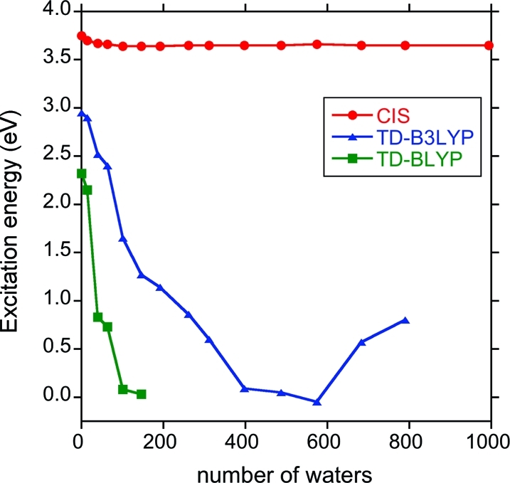
The first excitation energy (eV) of the PYP chromophore with increasing numbers of surrounding water molecules. Both TD-BLYP and TD-B3LYP exhibit spurious low-lying charge-transfer states. The geometry is taken from a single AMBER dynamics snapshot.

The recent theoretical work by Badaeva et al. examining the one and two photon absorbance of oligothiophene dendrimers was limited to results for the first three generations S1–S3, even though experimental results were available for S4.⁶⁵⁻⁶⁷ In Table 3, we compare our GPU accelerated results on the first bright excited state (oscillator strength >1.0) using TD-B3LYP within the TDA to the full TD-B3LYP and experimental results. Results within the TDA are comparable to those from full TD-B3LYP, for both energies and transition dipole moments. Our results for S4 show the continuing trend of decreasing excitation energy and increasing transition dipole moment with increasing dendrimer generation.

Table 3. Experimental and Calculated Vertical Transition Energies (eV) and Transition Dipole Moments (Debye) for the Lowest-Energy Bright State.

	Expta	TDA-TD-B3LYPb		TD-B3LYPc
	ΔE	ΔE	μge	ΔE	μge
S1	3.25	3.13	9.2	3.00	8.0
S2	3.25	2.98	10.6	2.92	10.1
S3	3.20	2.93	12.0	2.89	11.9
S4	3.19	2.83	13.3

^aExperimental results from refs (65 and 67).

^bGPU accelerated TD-B3LYP computed within the Tamm–Dancoff approximation.

^cTD-B3LYP results from ref (67).

Conclusions

We have implemented ab initio CIS and TDDFT calculations within the TeraChem software package, designed from inception for execution on GPUs. This allows full QM calculation of the excited states of large systems. The numerical accuracy of the excitation energies is shown to be excellent using mixed precision integral evaluation. A small percentage of cases require full double precision integration. For these occasional issues, we can easily switch to full double precision to achieve the desired convergence. The ability to use lower precision in much of the CIS and TDDFT calculation is reminiscent of the ability to use coarse grids when calculating correlation energies, as shown previously for pseudospectral methods.^79,82−85 Recently, it has also been shown(86) that single precision can be adequate for computing correlation energies with Cholesky decomposition methods which are closely related to pseudospectral methods.(87) Both quadrature and precision errors generally behave as relative errors, while chemical accuracy is an absolute standard (often taken to be 1 kcal/mol). Thus, coarser grids and/or lower precision can be safely used when the quantity being evaluated is itself small (and therefore less relative accuracy is required), as is the case for correlation and/or excitation energies.

For some of the smaller benchmark systems, we present speedups as compared to the GAMESS quantum chemistry package running over eight processor cores. The speedups obtained for CIS calculations range from 9 to 461 times, with increasing speedups with increasing system size. These speedup figures are not necessarily normative (other quantum chemistry packages might be more efficient), but we feel they give a good sense of the degree to which redesign of quantum algorithms for GPUs may be useful.

The increased size of the molecules that can be treated using our GPU-based algorithms exposes some failings of DFT and TDDFT. Specifically, the charge-transfer problem(16) of TDDFT and the delocalization problem(88) of DFT both seem to become more severe as the molecules become larger, especially for the case of hydrated chromophores with large numbers of surrounding quantum mechanical water molecules. It remains to be seen whether range-separated hybrid functionals^19,21 can solve these problems for large molecules, and we are currently working to implement these.

Supporting Information Available

CIS, BLYP, and B3LYP excitation energies, oscillator strengths, timings, number of CIS/TD iterations, geometry details. and Cartesian coordinates for the 22 structures used in this text. This material is available free of charge via the Internet at http://pubs.acs.org.

Funding Statement

National Institutes of Health, United States

References

- Foresman J. B.; Head-Gordon M.; Pople J. A.; Frisch M. J. J. Phys. Chem. 1992, 96, 135. [Google Scholar]
- Runge E.; Gross E. K. U. Phys. Rev. Lett. 1984, 52, 997. [Google Scholar]
- Gross E. K. U.; Kohn W. Phys. Rev. Lett. 1985, 55, 2850. [DOI] [PubMed] [Google Scholar]
- Casida M. E.Time Dependent Density Functional Response Theory for Molecules. In Recent Advances in Density Functional Methods; Chong D. P., Ed.; World Scientific: Singapore, 1995; pp 155. [Google Scholar]
- Casida M. E.; Jamorski C.; Casida K. C.; Salahub D. R. J. Chem. Phys. 1998, 108, 4439. [Google Scholar]
- Appel H.; Gross E. K. U.; Burke K. Phys. Rev. Lett. 2003, 90, 043005. [DOI] [PubMed] [Google Scholar]
- Hirata S.; Head-Gordon M.; Bartlett R. J. J. Chem. Phys. 1999, 111, 10774. [Google Scholar]
- Dreuw A.; Head-Gordon M. Chem. Rev. 2005, 105, 4009. [DOI] [PubMed] [Google Scholar]
- Burke K.; Werschnik J.; Gross E. K. U. J. Chem. Phys. 2005, 123, 062206. [DOI] [PubMed] [Google Scholar]
- Dallos M.; Lischka H.; Shepard R.; Yarkony D. R.; Szalay P. G. J. Chem. Phys. 2004, 120, 7330. [DOI] [PubMed] [Google Scholar]
- Kobayashi Y.; Nakano H.; Hirao K. Chem. Phys. Lett. 2001, 336, 529. [Google Scholar]
- Roos B. O. Acc. Chem. Res. 1999, 32, 137. [Google Scholar]
- Tokita Y.; Nakatsuji H. J. Phys. Chem. B 1997, 101, 3281. [Google Scholar]
- Krylov A. I. Annu. Rev. Phys. Chem. 2008, 59, 433. [DOI] [PubMed] [Google Scholar]
- Stanton J. F.; Bartlett R. J. J. Chem. Phys. 1993, 98, 7029. [Google Scholar]
- Dreuw A.; Weisman J. L.; Head-Gordon M. J. Chem. Phys. 2003, 119, 2943. [Google Scholar]
- Iikura H.; Tsuneda T.; Yanai T.; Hirao K. J. Chem. Phys. 2001, 115, 3540. [Google Scholar]
- Heyd J.; Scuseria G. E.; Ernzerhof M. J. Chem. Phys. 2003, 118, 8207. [Google Scholar]
- Tawada Y.; Tsuneda T.; Yanagisawa S.; Yanai T.; Hirao K. J. Chem. Phys. 2004, 120, 8425. [DOI] [PubMed] [Google Scholar]
- Rohrdanz M. A.; Herbert J. M. J. Chem. Phys. 2008, 129, 034107. [DOI] [PubMed] [Google Scholar]
- Rohrdanz M. A.; Martins K. M.; Herbert J. M. J. Chem. Phys. 2009, 130, 054112. [DOI] [PubMed] [Google Scholar]
- Grimme S. J. Comput. Chem. 2004, 25, 1463. [DOI] [PubMed] [Google Scholar]
- Grimme S. J. Comput. Chem. 2006, 27, 1787. [DOI] [PubMed] [Google Scholar]
- Vydrov O. A.; Van Voorhis T. J. Chem. Phys. 2010, 132, 164113. [DOI] [PubMed] [Google Scholar]
- Dion M.; Rydberg H.; Schroder E.; Langreth D. C.; Lundqvist B. I. Phys. Rev. Lett. 2004, 92, 246401. [DOI] [PubMed] [Google Scholar]
- For TDDFT, we are here referring to the adiabatic linear response formalism with presently available functionals.
- Maitra N. T.; Zhang F.; Cave R. J.; Burke K. J. Chem. Phys. 2004, 120, 5932. [DOI] [PubMed] [Google Scholar]
- Levine B. G.; Ko C.; Quenneville J.; Martinez T. J. Mol. Phys. 2006, 104, 1039. [Google Scholar]
- Jacquemin D.; Wathelet V.; Perpeate E. A.; Adamo C. J. Chem. Theory Comput. 2009, 5, 2420. [DOI] [PubMed] [Google Scholar]
- Warshel A.; Levitt M. J. Mol. Biol. 1976, 103, 227. [DOI] [PubMed] [Google Scholar]
- Virshup A. M.; Punwong C.; Pogorelov T. V.; Lindquist B. A.; Ko C.; Martinez T. J. J. Phys. Chem. B 2009, 113, 3280. [DOI] [PubMed] [Google Scholar]
- Ruckenbauer M.; Barbatti M.; Muller T.; Lischka H. J. Phys. Chem. A 2010, 114, 6757. [DOI] [PubMed] [Google Scholar]
- Polli D.; Altoe P.; Weingart O.; Spillane K. M.; Manzoni C.; Brida D.; Tomasello G.; Orlandi G.; Kukura P.; Mathies R. A.; Garavelli M.; Cerullo G. Nature 2010, 467, 440. [DOI] [PubMed] [Google Scholar]
- Schafer L.; Groenhof G.; Boggio-Pasqua M.; Robb M. A.; Grubmuller H. PLoS Comp. Bio. 2008, 4, e1000034. [DOI] [PMC free article] [PubMed] [Google Scholar]
- Kapasi U. J.; Rixner S.; Dally W. J.; Khailany B.; Ahn J. H.; Mattson P.; Owens J. D. Computer 2003, 36, 54. [Google Scholar]
- Compute Unified Device Architecture Programming Guide. NVIDIA CUDA, version 2.0; NVIDIA: Santa Clara, CA; http://developer.download.nvidia.com/compute/cuda/2_0/docs/NVIDIA_CUDA_Programming_Guide_2.0.pdf. Accessed August 1, 2010.
- Vogt L.; Olivares-Amaya R.; Kermes S.; Shao Y.; Amador-Bedolla C.; Aspuru-Guzik A. J. Phys. Chem. A 2008, 112, 2049. [DOI] [PubMed] [Google Scholar]
- Yasuda K. J. Chem. Theory Comput. 2008, 4, 1230. [DOI] [PubMed] [Google Scholar]
- Ufimtsev I. S.; Martinez T. J. J. Chem. Theory Comput. 2009, 5, 1004. [DOI] [PubMed] [Google Scholar]
- Asadchev A.; Allada V.; Felder J.; Bode B. M.; Gordon M. S.; Windus T. L. J. Chem. Theory Comput. 2010, 6, 696. [DOI] [PubMed] [Google Scholar]
- Ufimtsev I. S.; Martinez T. J. J. Chem. Theory Comput. 2009, 5, 2619. [DOI] [PubMed] [Google Scholar]
- Stone J. E.; Phillips J. C.; Freddolino P. L.; Hardy D. J.; Trabuco L. G.; Schulten K. J. Comput. Chem. 2007, 28, 2618. [DOI] [PubMed] [Google Scholar]
- Anderson J. A.; Lorenz C. D.; Travesset A. J. Comput. Phys. 2008, 227, 5342. [Google Scholar]
- Liu W.; Schmidt B.; Voss G.; Muller-Wittig W. Comput. Phys. Commun. 2008, 179, 634. [Google Scholar]
- Friedrichs M. S.; Eastman P.; Vaidyanathan V.; Houston M.; Legrand S.; Beberg A. L.; Ensign D. L.; Bruns C. M.; Pande V. S. J. Comput. Chem. 2009, 30, 864. [DOI] [PMC free article] [PubMed] [Google Scholar]
- PetaChem, LLC; PetaChem, LLC: Los Altos, CA; http://www.petachem.com.
- Ufimtsev I. S.; Martinez T. J. J. Chem. Theory Comput. 2008, 4, 222. [DOI] [PubMed] [Google Scholar]
- Ufimtsev I. S.; Martinez T. J. Comput. Sci. Eng. 2008, 10, 26. [Google Scholar]
- Shi G.; Kindratenko V.; Ufimtsev I. S.; Martinez T. J. Proceedings of the IEEE International Parallel and Distributed Processing Symposium (IPDPS), Atlanta, GA, April 19–23, 2010; IEEE: New York, 2010; p 1
- Grabo T.; Petersilka M.; Gross E. K. U. J. Mol. Struct. (THEOCHEM) 2000, 501–502, 353. [Google Scholar]
- Hirata S.; Head-Gordon M. Chem. Phys. Lett. 1999, 314, 291. [Google Scholar]
- Cordova F.; Doriol L. J.; Ipatov A.; Casida M. E.; Filippi C.; Vela A. J. Chem. Phys. 2007, 127, 164111. [DOI] [PubMed] [Google Scholar]
- Davidson E. R. J. Comput. Phys. 1975, 17, 87. [Google Scholar]
- CUBLAS Library; NVIDIA: Santa Clara, CA; http://developer.download.nvidia.com/compute/cuda/2_0/docs/CUBLAS_Library_2.0.pdf. Accessed August 1, 2010.
- Whitten J. L. J. Chem. Phys. 1973, 58, 4496. [Google Scholar]
- McMurchie L. E.; Davidson E. R. J. Comput. Phys. 1978, 26, 218. [Google Scholar]
- Ahmadi G. R.; Almlof J. Chem. Phys. Lett. 1995, 246, 364. [Google Scholar]
- Frisch M. J.; Johnson B.; Gill P. M. W.; Fox D.; Nobes R. Chem. Phys. Lett. 1993, 206, 225. [Google Scholar]
- Brown P.; Woods C.; McIntosh-Smith S.; Manby F. R. J. Chem. Theory Comput. 2008, 4, 1620. [DOI] [PubMed] [Google Scholar]
- Becke A. D. J. Chem. Phys. 1988, 88, 2547. [Google Scholar]
- Lebedev V. I.; Laikov D. N. Dokl. Akad. Nauk 1999, 366, 741. [Google Scholar]
- Murray C. W.; Handy N. C.; Laming G. J. Mol. Phys. 1993, 78, 997. [Google Scholar]
- Hancock J. M.; Gifford A. P.; Tonzola C. J.; Jenekhe S. A. J. Phys. Chem. C 2007, 111, 6875. [Google Scholar]
- Tao J.; Tretiak S. J. Chem. Theo. Comp. 2009, 5, 866. [DOI] [PubMed] [Google Scholar]
- Ramakrishna G.; Bhaskar A.; Bauerle P.; Goodson T. J. Phys. Chem. A 2007, 112, 2018. [DOI] [PubMed] [Google Scholar]
- Harpham M. R.; Suzer O.; Ma C.-Q.; Bauerle P.; Goodson T. J. Am. Chem. Soc. 2009, 131, 973. [DOI] [PubMed] [Google Scholar]
- Badaeva E.; Harpham M. R.; Guda R.; Suzer O.; Ma C.-Q.; Bauerle P.; Goodson T.; Tretiak S. J. Phys. Chem. B 2010, 114, 15808. [DOI] [PubMed] [Google Scholar]
- Yamaguchi S.; Kamikubo H.; Kurihara K.; Kuroki R.; Niimura N.; Shimizu N.; Yamazaki Y.; Kataoka M. Proc. Natl. Acad. Sci. U.S.A. 2009, 106, 440. [DOI] [PMC free article] [PubMed] [Google Scholar]
- Jorgensen W. L.; Chandrasekhar J.; Madura J. D.; Impey R. W.; Klein M. L. J. Chem. Phys. 1983, 79, 926. [Google Scholar]
- Nielsen I. B.; Boye-Peronne S.; El Ghazaly M. O. A.; Kristensen M. B.; Brondsted Nielsen S.; Andersen L. H. Biophys. J. 2005, 89, 2597. [DOI] [PMC free article] [PubMed] [Google Scholar]
- Becke A. D. Phys. Rev. A 1988, 38, 3098. [DOI] [PubMed] [Google Scholar]
- Lee C.; Yang W.; Parr R. G. Phys. Rev. B 1988, 37, 785. [DOI] [PubMed] [Google Scholar]
- Olivares-Amaya R.; Watson M. A.; Edgar R. G.; Vogt L.; Shao Y.; Aspuru-Guzik A. J. Chem. Theory Comput. 2010, 6, 135. [DOI] [PubMed] [Google Scholar]
- Yasuda K. J. Comput. Chem. 2008, 29, 334. [DOI] [PubMed] [Google Scholar]
- Of course, if the convergence threshold was made sufficiently small, all calculations would require double (or better) precision throughout.
- Luehr N.; Ufimtsev I. S.; Martinez T. J. J. Chem. Theory Comput. 2011, 7, 949. [DOI] [PubMed] [Google Scholar]
- Almlof J.; Faegri K.; Korsell K. J. Comput. Chem. 1982, 3, 385. [Google Scholar]
- Fewer points are included for the TD-BLYP timings in Figure 4 because the SCF procedure does not converge for the solvated PYP chromophore with a large number of waters or for the full PYP protein. This is due to the well-known problem with nonhybrid DFT functionals having erroneously low-lying charge-transfer states that can prevent SCF convergence.
- Ko C.; Malick D. K.; Braden D. A.; Friesner R. A.; Martinez T. J. J. Chem. Phys. 2008, 128, 104103. [DOI] [PubMed] [Google Scholar]
- Valiev M.; Bylaska E. J.; Govind N.; Kowalski K.; Straatsma T. P.; VanDam H. J. J.; Wang D.; Nieplocha J.; Apra E.; Windus T. L.; deJong W. A. Comput. Phys. Commun. 2010, 181, 1477. [Google Scholar]
- Grimme S.; Parac M. ChemPhysChem 2003, 4, 292. [DOI] [PubMed] [Google Scholar]
- Martinez T. J.; Carter E. A. J. Chem. Phys. 1993, 98, 7081. [Google Scholar]
- Martinez T. J.; Carter E. A. J. Chem. Phys. 1994, 100, 3631. [Google Scholar]
- Martinez T. J.; Carter E. A. J. Chem. Phys. 1995, 102, 7564. [Google Scholar]
- Martinez T. J.; Mehta A.; Carter E. A. J. Chem. Phys. 1992, 97, 1876. [Google Scholar]
- Vysotskiy V. P.; Cederbaum L. S. J. Chem. Theory Comput. 2010, 7, 320. [DOI] [PubMed] [Google Scholar]
- Martinez T. J.; Carter E. A.. Pseudospectral Methods Applied to the Electron Correlation Problem. In Modern Electronic Structure Theory, Part II; Yarkony D. R., Ed.; World Scientific: Singapore, 1995; p 1132. [Google Scholar]
- Cohen A. J.; Mori-Sanchez P.; Yang W. Science 2008, 321, 792. [DOI] [PubMed] [Google Scholar]
- Case D. A.; Cheatham T. E. III; Darden T.; Gohlke H.; Luo R.; Merz K. M. Jr.; Onufriev A.; Simmerling C.; Wang B.; Woods R. J. J. Comput. Chem. 2005, 26, 1668. [DOI] [PMC free article] [PubMed] [Google Scholar]
Associated Data
This section collects any data citations, data availability statements, or supplementary materials included in this article.
Data Citations