Detecting Rare and common Variants for complex traits: sibpair and odds ratio weighted sum statistics (SPWSS, ORWSS)

Abstract

It is generally known that risk variants segregate together with a disease within families but this information has not been used in the existing statistical methods for detecting rare variants. Here we introduce two weighted sum statistics that can apply to either genome-wide association data or resequencing data for identifying rare disease variants: weights calculated based on sibpairs and odd ratios, respectively. We evaluated the two methods via extensive simulations under different disease models. We compared the proposed methods with the weighted sum statistic (WSS) proposed by Madsen and Browning, keeping the same genotyping or resequencing cost. Our methods clearly demonstrate more statistical power than the WSS. In addition, we found using sibpair information can increase power over using only unrelated samples by more than 40%. We applied our methods to the Framingham Heart Study (FHS) and Wellcome Trust Case Control Consortium (WTCCC) hypertension datasets. Although we did not identify any genes as reaching a genome-wide significance level, we found variants in the candidate gene angiotensinogen (AGT) significantly associated with hypertension at P=6.9×10^-4, whereas the most significant single SNP association evidence is P=0.063. We further applied the odds ratio weighted method to the IFIH1 gene for type 1 diabetes in the WTCCC data. Our method yielded a P value of 4.82×10^-4, much more significant than that obtained by haplotype-based methods. We demonstrated that family data are extremely informative in searching for rare variants underlying complex traits, and the odds ratio weighted sum statistic is more efficient than currently existing methods.

Introduction

The recent meta-analyses of genome-wide association studies with sample sizes of over ten thousand have uncovered a large number of genetic variants underlying complex traits [Heid, et al. 2010; Lango Allen, et al. 2010]. Despite this success, the identified genetic variants usually have modest effect sizes and only account for a small proportion of the trait variation, resulting in the suggestion that many genetic variants, including both common and rare genetic variants, contribute little to phenotypic variation [Bansal, et al. 2010; Manolio, et al. 2009; Pritchard 2001]. In fact, recently many resequencing based studies of candidate genes have identified collections of rare variants associated with phenotypic variation [Bansal, et al. 2010]. Although a rare variant individually may make only tiny contributions to phenotypic variation, collectively rare variants may uncover a substantial proportion of missing heritability [Gibson 2010; Manolio, et al. 2009].

With recent advances, rare variants can be discovered and genotyped using next-generation sequencing technology. Directly testing many rare variants becomes possible and such experiments have led to the detection of multiple functional variants in IFIH1, NPC1L1, PCSK9, SLC12A3, SLC12A1 and KCNJ1 associated with type I diabetes, sterol absorption, plasma levels of LDL-C and blood pressure [Cohen, et al. 2005; Cohen, et al. 2006; Ji, et al. 2008; Nejentsev, et al. 2009]. In contrast to common variants, the power of traditional statistical methods to detect rare variants is usually poor and requires large sample sizes. Many statistical methods have been proposed to improve statistical power, and these methods can be divided into two categories.

The first category comprises methods based on collapsing or pooling a set of rare variants and testing them collectively [Han and Pan 2010; Li and Leal 2008; Madsen and Browning 2009; Morgenthaler and Thilly 2007; Morris and Zeggini 2010; Price, et al. 2010; Zawistowski, et al. 2010]. Excellent reviews of these methods can be found in the literature [Bansal, et al. 2010; Zawistowski, et al. 2010]. Cohen et al. proposed a method to compare the number of rare variants unique to either cases or controls using Fisher’s exact test [Cohen, et al. 2006] while Li and Leal proposed the combined multivariate and collapsing (CMC) method of pooling rare or functional variants and then comparing their distributions in cases and controls using a multivariate statistic [Li and Leal 2008]. Instead of pooling rare variants, Madsen and Browning[Madsen and Browning 2009] suggested the weighted sum statistic (WSS) that sums a weighted rare variant count in a gene or a region [Madsen and Browning 2009]. The weights are determined according to the variance of the variant frequency estimated in controls, with a larger weight given for a smaller allele frequency. A score is calculated for each individual and the scores are ranked for the cases and controls together. A test similar to the Wilcoxon rank sum test is applied to test for association between the set of rare variants and disease status via permutation. The WSS is more powerful than the CMC but for more computational cost. Price et al. [Price, et al. 2010] showed that the weights of the WSS are proportional to the log odds ratios of minor alleles and extended the WSS to a variable MAF threshold to maximize statistical power. A similar approach to the WSS, the cumulative minor-allele test (CMAT), was recently proposed and applied to sequencing data and samples using imputed probabilistic genotypes to alleviate the issue of uncertainty of genotype calls in low-coverage sequencing and imputation [Zawistowski, et al. 2010]. The power of the existing pooling methods is dependent on the threshold used to define a rare variant, which can result in misspecification of risk variants by either including neutral variants or excluding risk variants [Zawistowski, et al. 2010]. Price et al. [Price, et al. 2010] addressed this issue via a variable MAF threshold at the cost of more computation. This problem can be exacerbated for these pooling methods when both common and rare variants contribute to disease risk. The reason for this is that, when the MAF threshold is increased, many common neutral variants are also included - resulting in a dilution of association evidence. Thus, study designs are often restricted to analyzing the functional variants in a gene or a region assuming that many such variants are causal [Li and Leal 2008; Madsen and Browning 2009; Zawistowski, et al. 2010]. In addition, these methods only apply to unrelated samples, whereas family data have been shown to improve power to detect rare variants [Zhu, et al. 2010].

The second category of methods compares haplotype frequencies between cases and controls [Feng and Zhu 2010; Guo and Lin 2008; Li, et al. 2010; Zhu, et al. 2005; Zhu, et al. 2010]. A basic assumption is that the haplotypes created by the common and rare variants are able to tag multiple rare ungenotyped variants. It is clear that rare variants are not usually well tagged by common variants [Durbin, et al. 2010] and thus the haplotype based methods only work for identifying rare variants with MAF >0.5% [Li, et al. 2010]. Similar to the rare variant pooling methods, the haplotype based methods either collapse rare risk haplotypes [Zhu, et al. 2010] or sum the haplotype scores weighted by emphasizing the haplotypes with a low frequency in controls [Li, et al. 2010]. The haplotype based methods can be applied to the data collected by genome-wide association studies [Feng and Zhu 2010]. However, to apply haplotype based methods, haplotype phases have to be inferred, which adds a substantial computational burden. However, since we only need to infer the haplotype phases once in any data analysis, the computation is still within feasible limits. When risk variants are extremely rare (<0.5%), the power of haplotype based methods can be low.

In this article, we develop a sibpair based weighted sum statistic to detect both rare and common risk variants residing in a gene or a genomic region. We argue that risk variants will cosegregate with a disease in families and the risk variants will be enriched in ascertained families such as affected sibpairs, as demonstrated in Zhu et al. [Zhu, et al. 2010]. We then propose a weighted method for summation of the risk variants using either affected or discordant sibpairs. We theoretically show that the weights are proportional to the effect sizes of risk variants. This pooling method does not require choosing a threshold of MAF for defining whether a variant is rare, which is necessary for all the existing weighted methods. It can be applied to sequencing or GWAS data. In addition, we also suggest that directly using the odds ratio of a variant as a weight in the WSS can be more powerful than the original WSS. Our methods are not affected by the directionality of effect. Since the WSS is more powerful than other existing methods when an appropriate MAF threshold is applied, we compared the power of our methods with the WSS using the best threshold on case-control sequencing datasets simulated based on HapMap ENCODE data [Frazer, et al. 2007]. We did not directly compare our methods with the haplotype based methods in the simulation study, but we performed the comparison by applying them to real data. As proof of principle, we applied our methods to the analysis of hypertension and type 1 diabetes using the Framingham Heart Study data [Levy, et al. 2009] and the Wellcome Trust Case Control Consortium (WTCCC) data[2007].

Methods

Assume we will test the association of genetic variants and disease status in a candidate gene or a genomic region. For genome-wide data, such as whole genome or whole exon resequencing data, we can always partition the data into genes or genomic regions and test the association in each gene or genomic region [Zhu, et al. 2010]. Our test procedure is similar to the WSS of Madsen and Browning [Madsen and Browning 2009]. Assume we collected N_D cases and N_C controls. Let x_ij be the number of minor alleles at the j^th SNP carried by the i^th individual (both cases and controls) in a gene or a genomic region, where L SNPs are genotyped and j = 1, 2,…, L. We define the genetic score

$$X_i={\sum }_{j=1}^L{w}_j{x}_{\mathit{ij}},$$ (1)

for the i^th individual, where w_j is the weight for the j^th SNP. (If the weight w_j is the inverse of the j^th SNP’s variance estimated in controls, this is equivalent to the WSS. We will discuss how to calculate the weights later.) We then rank the genetic scores and calculate the sum of the ranks for cases as

$$X={\sum }_{i\in \mathit{Cases}}\mathit{rank}\left(X_i\right)$$ (2)

We chose the Wilcoxon rank sum test because the individuals’ genetic scores X_i can be severely skewed and outliers may exist depending on the number of rare variants an individual carries. Further, our weight calculation described later is also dependent on the minor allele frequency (MAF) in controls. We then use the same permutation strategy as the WSS [Madsen and Browning 2009] to assess the power and type I error rate. That is, we permute disease status among individuals 1,000 times to compute the statistic X in equation (2) as $X_1^{\ast },X_2^{\ast },\dots ,X_{1000}^{\ast }$. We next calculate the sample mean μ̂ and standard deviation σ̂ of $X_1^{\ast },X_2^{\ast },\dots ,X_{1000}^{\ast }$. The test statistic is defined as $Z=\frac{X-\widehat{\mu }}{\widehat{\sigma }}$, which follows approximately a standard normal distribution. In what follows, we propose three different weighting methods based respectively on affected sibpairs, discordant sibpairs and unrelated case-controls. We call our methods the Sibpair Weighted Sum Statistic (SPWSS) and the Odds Ratio Weighted Sum Statistic (ORWSS). In contrast to the requirement for existing weighted methods, the proposed weighted methods do not require setting a threshold for the MAF.

Defining the weight of a variant

Previously, we demonstrated that rare risk variants will be enriched in ascertained families such as affected sibpairs [Zhu, et al. 2010]. We thus use families, such as affected sibpairs or discordant sibpairs, to define the weights. We will show that with the same size of genotype effect, using family data can greatly increase statistical power in detecting rare risk variants. We make the assumption that a minor allele is either a risk allele or neutral. We note in the Discussion section that similar methods can be applied to detect protective variants.

(1) Affected sibpair design

We assume there are N_sib affected sibpairs. Assume a SNP has two alleles A and a, and A always refers to the minor allele for all the SNPs we are examining. We let ~ represent either the A or a allele at any SNP. Denote the i^th sibpair’s genotypes of the L SNPs as g_i = ((g_i11, g_i21), (g_i12, g_i2L),…, (g_i1L, g_i2L)), where (g_i1j, g_i2j) refers to the j^th SNP’s genotypes for the i^th sibpair. We do not differentiate the first or second sib here. Our idea is that if A at the j^th SNP is a risk allele, the weight for this allele A should be proportional to the ratio of the risk of both affected sibs carrying A to that in the general population. In this case, we assume the weight will only depend on the alleles carried at the j^th SNP. That is, if both affected sibs carry A at the j^th SNP, the weight of A at this SNP is proportional to

$$\frac{P(\mathit{both\; sibs\; are\; affected}|(g_{i1j},g_{i2j})=(A~,A~))}{p(\mathit{both\; sibs\; are\; affected})}=\frac{P((g_{i1j},g_{i2j})=(A~,A~)|\mathit{both\; sibs\; are\; affected})}{{\mathit{\varphi }}_1},$$ (3)

Where ϕ₁ = P((g_i1j, g_i2j) = (A ~, A ~)). If one sib carries A at the j^th SNP and the other does not, the weight of A is dependent on how many other sites have an A allele carried by the other affected sib. That is, the weight is proportional to

$$\frac{P[\mathit{both\; sibs\; are\; affected}|(g_{i1j},g_{i2j})=(A~,\mathit{aa}),\mathit{A\; present\; at\; other\; sites}\mathrm{of\; sib}2]}{p(\mathit{both\; sibs\; are\; affected})}=\frac{P[(g_{i1j},g_{i2j})=(A~,\mathit{aa}),\mathit{A\; present\; at\; other\; sites}\mathrm{of\; sib}2|\mathit{both\; sibs\; are\; affected}]}{{\mathit{\varphi }}_2},$$ (4)

where ϕ₂ = P[(g_i1j, g_i2j) = (A ~, aa), A present at other sites of sib 2]. In Equation (4) we always assume the first sib carries allele A when examine the other sibs carrying allele A at the j^th marker.

Based on equations (3) and (4), we can define a genotype score for each SNP in a sibpair. That is, for the i^th affected sibpair and the j^th SNP, we define the genotype score as

$${\tilde{g}}_{\mathit{ij}}=\{\begin{array}{ll}\frac{1}{{\mathit{\varphi }}_1}& ,\mathit{when}\left(g_{i1j},g_{i2j}\right)=\left(A~,A~\right)\\ \frac{L_0}{2L{\mathit{\varphi }}_2}& ,\mathit{when}\left(g_{i1j},g_{i2j}\right)=\left(A~,\mathit{aa}\right),\mathit{and}{L}_0\mathit{of\; the\; other\; SNPs\; carry\; an\; A\; allele}\mathrm{for\; sib}2\\ 0& ,\mathit{otherwise}\end{array}$$ (5)

In equation (5) the second term was divided by 2 because either one of the sibs may carry the A~ genotype at the j^th SNP. We give the formulas for calculating ϕ₁ and ϕ₂ in appendix A. ϕ₁ is the function of one A allele frequency at the j^th SNP and ϕ₂ is a function of the other A allele frequencies at the other SNPs; ϕ₂ is dependent on the second sib’s genotypes at L SNPs. We evaluate them using the MAFs of the SNPs in the controls. For the j^th SNP, we then calculate ${\gamma }_j=\frac{1}{N_{\mathit{sib}}}\sum _{i=1}^{N_{\mathit{sib}}}{\tilde{g}}_{\mathit{ij}}$, which is the average of the genotype scores defined in equation (5). Under the alternative hypothesis, in which only a subset of variants are risk variants, we would expect these variants to be outliers. We thus define the weight for the j^th SNP to be

$$w_j=\{\begin{array}{ll}{\gamma }_j& ,\mathit{if}{\gamma }_j>\overline{\gamma }+c\sigma \\ 0& ,\mathit{otherwise}\end{array},$$ (6)

where γ̄ and σ is the mean and standard deviation calculated from γ_j, j = 1,…L, and c is a pre-specified parameter. (The power of our test proposed later should be dependent on the choice of c. In our simulations, we tried different values of c and found these different values have only a slight effect on the power (Supplementary Tables 1 and 2). We then use these weights in an association test based on equation (2). We term this method of using weights defined by affected sibpairs as SPWSS_AA.

(2) Discordant sibpair design

For discordant sibpairs, the first sib is always chosen to be affected and the second is always unaffected. We assume there are N_sib discordant sibpairs. The weight of allele A at the j^th SNP should be proportional to

$$\frac{P(\mathit{sib}1\mathit{is\; affected\; and\; sib}2\mathit{is\; not}|(g_{i1j},g_{i2j})=(A~,\mathit{aa}))}{p(\mathit{sib}1\mathit{is\; affected\; and\; sib}2\mathit{is\; not})}=\frac{P(g_{i1j},g_{i2j})=(A~,\mathit{aa})|\mathit{sib}1\mathit{is\; affected\; and\; sib}2\mathit{is\; not}}{{\mathit{\varphi }}_3},$$ (7)

Where ϕ₃ = P((g_i1j, g_i2j) = (A ~, aa)). For the i^th discordant sibpair and the j^th SNP, we define the genotype score to be

$${\tilde{g}}_{\mathit{ij}}=\{\begin{array}{ll}\frac{1}{{\mathit{\varphi }}_3}& ,\mathit{when}\left(g_{i1j},g_{i2j}\right)=\left(A~,\mathit{aa}\right)\\ 0& ,\mathit{otherwise}\end{array}.$$

We give the formula for calculating ϕ₃ in appendix A. ϕ₃ is a function of the MAF of the j^th SNP in the population and we evaluate it using the MAF in the controls. In the same way as for affected sibpairs, we define the weights for discordant sibpairs as in equation (6). We then use these weights in an association test based on equation (2). We call this method of using weights defined by discordant sibpairs as SWSS_AU.

Case-control data

Most studies only recruit unrelated cases and controls and we here propose a weighted method that for this design does not require a threshold for defining rare variants. Price et al [Price, et al. 2010] demonstrated that the weights proposed by Madsen and Browning [Madsen and Browning 2009] is proportional to the log odds ratio for a variant. In addition, a coefficient in a logistic regression is equivalent to the logarithm of the corresponding odds ratio. We therefore directly use the odd ratio of a variant as the weight for that variant, rather than the variance estimated in controls. That is, we calculate the odds ratio between allele A at the j^th SNP and a disease status using a 2 × 2 table. Since we are interested in rare variants and the corresponding 2 × 2 table may consist of entries with 0 observations, we applied the amended estimator of the odds ratio by adding 0.5 to each cell. It has been suggested that the amended estimator of the odds ratio behaves well [Agresti 2002]. We now define γ_j as the logarithm of the amended odds ratio testing for the association of allele A at the j^th SNP using all the cases and controls. In the same way as for affected sibpairs and discordant sibpairs, we define the weight for the j^th SNP as

$$w_j=\{\begin{array}{ll}{\gamma }_j& ,\mathit{if}{\gamma }_j>\overline{\gamma }+c\sigma \mathit{or}{\gamma }_j<\overline{\gamma }-c\sigma \\ 0& ,\mathit{otherwise}\end{array},$$ (8)

where σ is the standard deviation calculated from γ_j, j = 1,…L, c is a parameter and γ̄ is the mean. We call this method of using odds ratio weights, defined for unrelated cases and controls, as ORWSS (Odds ratio weighted sum statistic).

Simulating Data

The HapMap ENCODE project resequenced 10 genomic regions of 500kb for samples from three populations: CEU, YRI and JPT/CHB [Birney, et al. 2007]. We downloaded the genotype data in ENm010 on 7p15.2 from the HapMap website (www.hapmap.org). We inferred haplotypes using the software Beagel [Browning and Browning 2007] in each population separately. To increase the number of rare variants we combined the CEU, YRI and JPT/CHB samples together. We expect that most of the variants in this region have already been discovered. After dropping the monomorphic sites, there are 808 SNPs comprising 529 unique haplotypes for a total of 269 individuals. Table 1 lists the distribution of rare variants in this region. We believe this size of genomic region should be comparable with a gene or a region where association can be tested.

Table 1.

The rare variant distribution in ENm010 on 7p15.2 in HapMap ENCODE data

	Minor allele frequency p
	0.002	0.005	0.0075	0.01	0.02	0.03	0.04	0.05
# of SNPs with MAF < p	60	108	157	173	233	270	305	333
# of unique Haplotypes the rare SNPs fall in	53	117	208	250	364	453	484	507

To simulate cases and controls, we set the cumulative frequency of the risk alleles at 10%. We assumed two disease risk allele frequency models: 1) only the variants with MAF<2% can be risk variants; 2) there is one common variant with MAF between 5% and 8% and the rest of the risk variants have MAF<2%. For model 1, we randomly drew risk variants with MAF<2% until the accumulated frequency of haplotypes in which the sampled variants fell reached 10%. This procedure led to an average of 16±7.7 variants that are disease variants. For the second case, we first randomly picked a common variant with MAF between 5% and 8%. We then randomly sampled the rest as rare variants until the accumulated haplotype frequency reached 10%. This procedure led to an average of 6.3±5.5 variants being risk variants. We considered the haplotypes in which the sampled risk variants fell as the risk haplotypes and we further assumed their effects on the phenotype are the same, i.e. that penetrance is only dependent on how many risk haplotypes an individual carries. We then simulated the cases, controls and sibpairs as described in Zhu et al. [Zhu, et al. 2010]. Briefly, an individual’s genotype was simulated by randomly drawing two haplotypes according to the haplotype frequencies. Disease status was simulated based on the penetrances, given the haplotypes, according to three modes of inheritance: dominant, additive and recessive. To simulate affected sibpairs, we independently simulated two individuals as the parents and then randomly transmitted one of the two haplotypes from each parent to his/her offspring. We kept generating sib pairs from parent-pairs until we had generated enough affected or discordant sibpairs.

Results

Type I error

Since we used the approximation strategy for permutation testing discussed in the Method section in order to save computation time, we first evaluated the type I error rate for the proposed methods and the WSS. We simulated the data under the null hypothesis: that is we let the relative risk rr = 1.0 for any genotype an individual carries. Our simulation results demonstrate that the type I error rates are reasonable for the proposed methods as well as for the WSS (Table 2).

Table 2.

Type I error rate for the SPWSS, ORWSS, WSS when risk variants are only rare and when risk variants include both rare and common variants. All the type I error rates were calculated based on 5,000 replications.

		α = 0.05		α = 0.01		α = 0.005		α = 0.001
#of Sibpairs	design	SPWSS	ORWSS	SPWSS	ORWSS	SPWSS	ORWSS	SPWSS	ORWSS
200	affected	0.0494	0.0482	0.0084	0.0084	0.0044	0.0042	0.0010	0.0004
	discordant	0.0536	0.0438	0.0102	0.0080	0.0054	0.0046	0.0006	0.0008
400	affected	0.0525	0.0468	0.0110	0.0059	0.0056	0.0034	0.0015	0.0002
	discordant	0.0482	0.0468	0.0092	0.0090	0.0040	0.0052	0.0000	0.0000

Power

Using the simulation procedure described above, we generated 2,000 cases, 2,000 controls and 200 affected sibpairs for the SPWSS using affected sibpairs (SPWSS_AA). For a fair comparison, we simulated 2,400 cases and 2,000 controls for both the ORWSS and the WSS. Similarly, we generated 2,000 cases, 2,000 controls and 200 discordant sibpairs for the SPWSS using discordant sibpairs (SPWSS_AU). For comparison, we simulated 2,200 cases and 2,200 controls for both the ORWSS and the WSS. Thus, the total genotyping effort would be the same for the compared methods. The power was calculated at the significance level α=10^-6 based on 1,000 replications. Three disease models were assumed: Dominant, Additive and Recessive. We assumed all the risk allele frequencies were less than 0.02, with a cumulative risk allele frequency of 10%. In each replication, we sampled risk variants until the cumulative sampled risk allele frequency reached 10%. Thus, the risk variants in the different replications were not fixed. This procedure allows us to evaluate a wide range of risk variant distributions in a region. Figure 1 presents the power of the three different methods: the SPWSS, ORWSS and WSS. When using the weights based on 200 affected sibpairs (Figure 1 top panel), the SPWSS is the most powerful method, followed by the ORWSS, for all three modes of inheritance. When the relative risk is 2.0, the SPWSS_AA has 25% more power than the ORWSS, and 50% more than the WSS, for a dominant disease model. For an additive model, the SPWSS has 40% more power when the relative risk is 3.0. There is no power for any of the three methods for a recessive model. For the WSS, we used a threshold 0.02, which represents the best threshold since the MAFs for all the true risk variants were less than 2%. Thus, the power for the WSS should represent the best power it can attain. When comparing the weights based on 200 discordant sibpairs (Figure 1 bottom panel), for a dominant model the ORWSS is the most powerful and SPWSS_AU and the WSS have similar power. For an additive model, the three methods have comparable power. We did not observe any power for a recessive model for any of the three methods. When we increase the number of sibpairs for the SPWSS to 400, and correspondingly the number of cases and controls for the ORWSS and WSS, the power pattern is similar to that using 200 sibpirs for calculating the weights (Supplementary Figure 2).

Figure 1.

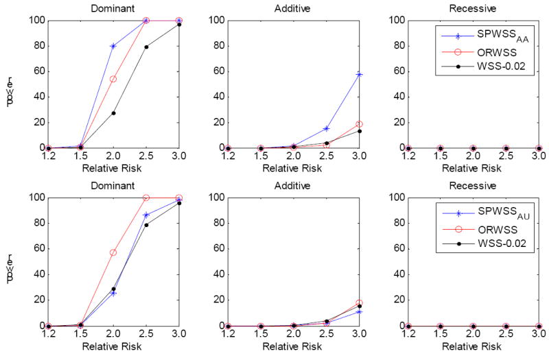
Comparison of power for different relative risks. All the risk allele frequencies are less than 0.02, with a cumulative risk allele frequency of 10%. The power was calculated at significance level α=10^-6 based on 1,000 replications. Three disease modes have been assumed: Dominant, Additive and Recessive. All the risk alleles were treated the same. Top panel: for SPWSS_AA, we simulated 200 affected sibpairs for calculating the weights, and 2,000 cases and 2000 controls for the association test. For ORWSS and WSS, we simulated 2,400 cases and 2,000 controls for the association test. Bottom panel: for SPWSS_AU, we simulated 200 discordant sibpairs for calculating the weights, and 2,000 cases and 2000 controls for the association test. For ORWSS and WSS, we simulated 2,200 cases and 2,200 controls for the association test. For WSS, we used the threshold 0.02 to define rare variants; that is, all the risk variants belong to the rare variant group.

It is possible that there may be both common and rare disease variants in a gene or a genomic region [Momozawa, et al. 2011]. We thus investigated the power performance for the three methods when disease variants include both common (MAF between 5% and 8%) and rare (MAF<2%) variants. We applied the same procedure as before. However, we first sampled a common disease variant and then the rest were rare disease variants. We set the cumulative risk allele frequency at ~10%. For the WSS, we used three MAF thresholds: 0.02, 0.05 and 0.08, to determine if a SNP should be filtered out. We expected the threshold 0.08 to have the best power for the WSS because all the disease variants will then be included in the analysis. Figure 2 presents the power of the three methods when 200 sibpairs were used for weight calculation for the SPWSS. We observed that the power of the SPWSS and ORWSS remains. However, the power of the WSS is critically dependent on the MAF threshold. As expected, the WSS with the threshold 0.08 gives the best power, followed by the threshold 0.05. The power decreases substantially for the threshold 0.02, with over 30% for a dominant model. The results are similar when the sample size is increased (Figure 3).

Figure 2.

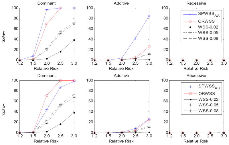
Comparison of power for different relative risk. For each replication, we assumed there is a common risk variant (MAF is between 0.05 and 0.08) and the rest risk variants are rare (MAF<0.02), with a cumulative risk allele frequency of 10%. The power was calculated at significance level α=10^-6 based on 1,000 replications. Three disease models have been assumed: Dominant, Additive and Recessive. All the risk alleles were treated the same. Top panel: for SPWSS_AA, we simulated 200 affected sibpairs for calculating the weights, and 2,000 cases and 2000 controls for the association test. For ORWSS and WSS, we simulated 2,400 cases and 2,000 controls for the association test. Bottom panel: for SPWSS_AU, we simulated 200 discordant sibpairs for calculating the weights, and 2,000 cases and 2000 controls for the association test. For ORWSS and WSS, we simulated 2,200 cases and 2,200 controls for the association test. For WSS, we used different thresholds: 0.02, 0.05 and 0.08 to define the rare variants.

Figure 3.

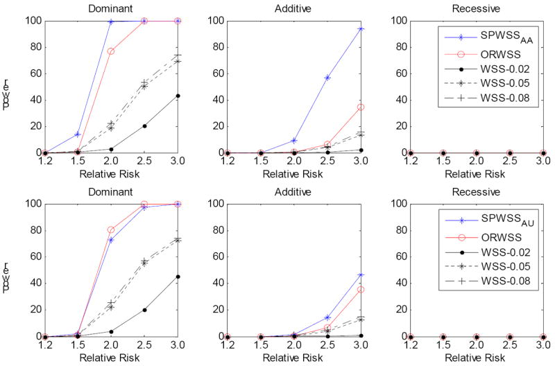
Comparison of power for different relative risk. For each replication, we assumed there is a common risk variant (MAF is between 0.05 and 0.08) and the rest risk variants are rare (MAF<0.02), with a cumulative risk allele frequency of 10%. The power was calculated at significance level α=10^-6 based on 1,000 replications. Three disease models have been assumed: Dominant, Additive and Recessive. All the risk alleles were treated the same. Top panel: for SPWSS_AA, we simulated 400 affected sibpairs for calculating the weights, and 2,000 cases and 2000 controls for the association test. For ORWSS and WSS, we simulated 2,800 cases and 2,000 controls for the association test. Bottom panel: for SPWSS_AU, we simulated 400 discordant sibpairs for calculating the weights, and 2,000 cases and 2000 controls for the association test. For ORWSS and WSS, we simulated 2,400 cases and 2,400 controls for the association test. For WSS, we used different thresholds: 0.02, 0.05 and 0.08 to define the rare variants.

The power is also dependent on the number of sibpairs used in computing the weights, as suggested in our previous study [Zhu, et al. 2010]. We thus compared the power of 200 sibpairs, 2000 case and 2000 controls with 400 sibpairs, 1800 case and 1800 controls. Thus, the total sample sizes are the same. Figure 4 presents the power for both affected sibpairs and discordant sibpairs. In general, we observed the power using different numbers of sibpairs for weight calculations is similar, with slightly more power with increasing sibpairs. This result also suggests the importance of using more family data in rare variant association analysis.

Figure 4.

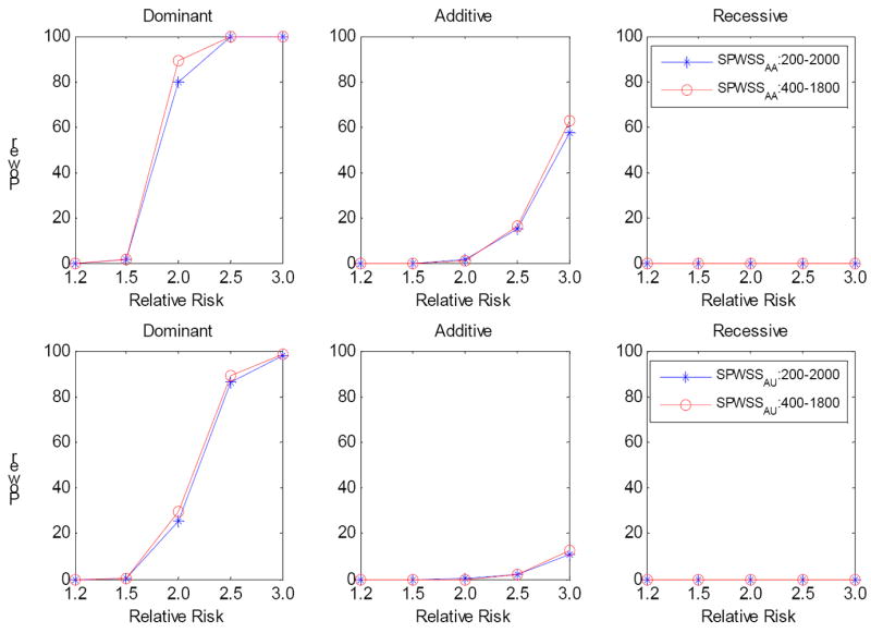
Comparison of power for SPWSS when the total sample size is fixed. The power was calculated at significance level α=10^-6 based on 1,000 replications. Three disease models have been assumed: Dominant, Additive and Recessive. All the risk alleles were treated the same. We compared 200 sibpairs, 2000 cases and 2000 controls with 400 sibpairs, 1800 cases and 1800 controls. Top panel: SPWSS_AA; Bottom panel: for SPWSS_AU.

In the above analysis we chose c=1.64. We then repeated the same analysis but with c=1.28. Supplementary figure 2 and 3 show the power for the different c values. We observed the power is essentially the same for the different values of c.

Application to the Framingham Heart Study and Wellcome Trust Case Control Consortium data

Our simulation study suggests both the SPWSS and ORWSS can be more powerful than the WSS. In addition, the SPWSS and ORWSS do not require a threshold to filter out the common variants. As proof of principle for the methods, we applied the SPWSS and ORWSS to the Framingham Heart Study (FHS)[Levy, et al. 2009] and Wellcome Trust Case Control Consortium (WTCCC) hypertension dataset [2007]. We applied the same QC as did Feng and Zhu [Feng and Zhu 2010]. For the FHS data, we further performed a Mendelian inheritance consistency check. We set a genotype as missing if a Mendelian inheritance error was identified. We next kept the overlapping SNPs genotyped in both the WTCCC and the FHS, and these SNPs were mapped to genes based on map annotations provided by Affymetrix 6.0 GeneChip (https://www.affymetrix.com/support/technical/annotationfilesmain.affx). We only analyzed the SNPs in 13,005 genes. We identified a total of 265 affected sibpairs in the FHS data and these affected sibpairs were used for the weight calculation in the SPWSS. The association tests were performed using WTCCC hypertension cases and common controls. For comparison, we performed the ORWSS and WSS using the WTCCC data only. Because both the SPWSS and ORWSS required calculating the mean and standard deviation of the test statistics from permutations, it is possible for all the SNP weights in equations (6) and (8) to be 0 when only a few SNPs are available in a gene, resulting in underestimated variances of the test statistics. Thus, we directly used the γ_j in equations (6) and (8) as the weights when the number of SNPs in a gene was less than 20. We chose 20 SNPs to ensure that we will have at least one SNP with a weight not equal to 0. There were 9,446 genes having less than 20 SNPs. We set the MAF at 0.05 to filter out the common SNPs for the WSS. When there is only one SNP with MAF close to 0.05, it is also likely that all the SNP weights in the WSS are 0 in the permutations, resulting in an underestimated variance of the test statistic. In such cases these genes were excluded in the WSS analysis. Overall, we did not observe any gene reaching significance by any of the three methods after correcting for 13,005 tests.

We next focused on the association between hypertension and four genes: angiotensinogen (AGT), renin (REN), angiotensin I-converting enzyme (ACE), and the angiotensin II receptor, subtype 1 (AGTR1), which encodes components of the renin-angiotensin system (RAS). RAS plays a critical physiological role in the cardiovascular system and the four genes are considered as candidate genes for hypertension [Zhu, et al. 2003]. The P-values for the SPWSS, ORWSS and WSS are shown in Table 3. The P-values of AGT for the SPWSS and ORWSS are 2.56×10^-3 and 4.76×10^-3 but not significant for the WSS (P=0.556). There are 8 SNPs being genotyped in AGT and Table 4 presents the single SNP association tests with hypertension in the WTCCC data. We did not observe any significant association evidence in the single SNP association analysis, although four of eight SNPs have P-values less than 0.1. We examined the linkage disequilibrium (LD) among the 8 SNPs in AGT and found that three of them (rs7555650, rs7549009 and rs4628514) are in almost perfect LD (Table 5). We then kept only rs7555650 and performed the SPWSS, ORWSS and WSS again. The significance association evidence for the SPWSS was further improved (P value=6.91×10^-4) but for the ORWSS it remained similar (P value=4.97×10^-3). Thus, our methods identified multiple variants in this gene contributing to the association evidence for AGT. When we applied the two-stage haplotype grouping (HG) method [Zhu, et al. 2010], we obtained the P-value 0.011, which is significant after correcting for four tests.

Table 3.

P values for the association of rare variants in four RAS genes with hypertension in the WTCCC dataset. The weights for SWSS were calculated based on affected sibpairs in the FHS dataset.

Gene	# of SNP	SPWSS	ORWSS	WSS	HG
ACE	3	0.877	0.893	1.0	1.0
AGT	8	2.56×10-3	4.76×10-3	0.556	0.011
AGT1	6	6.91×10-4	4.97×10-3	0.492	-
AGTR1	45	0.147	0.972	0.356	0.36
REN	4	0.265	0.432	1.0	1.0

¹rs7549009 and rs4628514 were excluded because of the perfect LD with rs7555650.

Table 4.

The results of the single SNP association of the eight variants in AGT with hypertension in WTCCC data.

AGT variants	Minor Allele	MAF in Cases	MAF in Controls	OR	P-value
rs1926723	C	0.0891	0.0789	1.14	0.0732
rs11122577	A	0.1733	0.1623	1.08	0.1566
rs2071406	C	0.0362	0.0338	1.08	0.5185
rs2071404	A	0.1158	0.1049	1.12	0.0925
rs7555650	T	0.1031	0.0925	1.13	0.0838
rs7549009	A	0.1038	0.0957	1.09	0.1917
rs4628514	C	0.1037	0.0960	1.09	0.2112
rs4847008	T	0.2187	0.2031	1.10	0.0631

Table 5.

r² values of 8 SNPs in AGT.

SNPs	rs1926723	rs11122577	rs2071406	rs2071404	rs7555650	rs7549009	rs4628514
rs11122577	0.018
rs2071406	0.003	0.007
rs2071404	0.011	0.025	0.004
rs7555650	0.778	0.02	0.003	0.012
rs7549009	0.776	0.021	0.003	0.013	0.998
rs4628514	0.777	0.021	0.003	0.013	0.998	1.0
rs4847008	0.323	0.052	0	0.382	0.407	0.411	0.411

Application to the IFIH1 gene in the WTCCC type 1 diabetes data

Multiple common and rare variants in the IFIH1 gene have been identified as contributing to the risk of type 1 diabetes (T1D). Li et al. [Li, et al. 2010] analyzed six polymorphisms in IFIH1 genotyped in the WTCCC T1D data but excluded the common SNP rs1990760, which has already been identified as associated with T1D [Nejentsev, et al. 2009]. Using the weighted haplotype and imputation-based tests (WHalT), Li et al. found much stronger association evidence between the haplotypes consisting of these six SNPs and T1D than the existing methods, including the WSS [Li, et al. 2010], with the smallest P value 4.31×10^-3. We then applied the ORWSS and WSS to the same data because only unrelated samples are available. However, SNP rs41463049 was not available in our data, so we applied the ORWSS and WSS to only the other five SNPs. Because there are only five SNPs available, the odds ratio for each SNP was used as the weight without further filtering out SNPs. The P-values for the ORWSS and WSS are 4.82×10^-4 and 0.49, respectively. We also applied the haplotype grouping method we previously developed [Feng and Zhu 2010; Zhu, et al. 2010]. Since the haplotypes created by the five SNPs seem to have a protective effect, we grouped haplotypes showing a protective effect together and then performed an association test based on 10,000 permutations. We obtained a P-value of 0.0021 for the haplotype grouping test, slightly more significant than that by Weighted haplotype and Imputation-based tests. This result clearly demonstrates that the ORWSS can be more powerful than currently existing methods in searching for the rare variants affecting complex diseases, and the weights by the odds ratio is more efficient than the weights by the MAF.

Discussion

By the motivation that rare disease variants will be enriched in family data [Feng and Zhu 2010], we developed a sibpair based weighted sum statistic (SPWSS) to detect rare variants associated with complex traits. Further, we suggested that using an odds ratio rather than MAF as a weight can improve power for detecting rare disease variants. These methods can be applied to either resequencing data or GWAS data. Our methods do not require a MAF threshold, which is critical for the existing methods. Thus, our methods also have power to detect genes when both common and rare variants exist in the data. In fact, our methods filter out variants according to the weights calculated from either sibpairs or odds ratios. The reason for this is that, if a variant is a risk variant, we would choose a weight for this variant to be proportional to the relative risk for sibs carrying the risk allele, or to the odds ratio of carrying the risk allele. If a variant is neutral, the relative risk for sibpairs or the odds ratio of a minor allele is close to 1. We expect the weights of risk variants to fall in the extreme tail of the weight distribution. For a MAF threshold based method such as the WSS, noise can be introduced by a predefined MAF threshold because of the neutrality of many rare variants. In addition, a true risk variant may have a MAF larger than a predefined MAF threshold. In this case, a MAF threshold based method such as the WSS will lose statistical power. Thus, our proposed methods have substantial advantages over the existing methods.

We compared the SPWSS with weights calculated from affected and discordant sibpairs via simulated data for a variety of disease models. We found that the SPWSS based on affected sibpairs is more powerful than that based on discordant sibpairs. This is not surprising, because rare variants are more frequent in affected sibpairs than in discordant sibpairs. We thus suggest that in practice affected sibpairs should be used when they are available. Since traditional linkage studies have collected a large number of affected sibpairs for a variety of diseases, we argue that the affected sibpair method should be convenient in practice. In addition, family data have a better chance to detect genotype errors than unrelated samples. Furthermore, this method can also be used to search for protective rare variants by defining weights based on unaffected sibpairs. Our simulations also demonstrated that the SPWSS using affected sibpairs can dramatically improve statistical power over the methods based on unrelated methods, suggesting family data may be extremely useful for detecting rare disease variants.

We assumed that the penetrance is a constant and is only dependent on how many of an individual’s haplotypes carry risk variants, rather than the total number of risk variants an individual carries. In practice, different rare risk variants may have different disease risks. Some of them may even be protective. Han and Pan [Han and Pan 2010] demonstrated that the power of the WSS [Madsen and Browning 2009] and CMC [Li and Leal 2008] can be substantially reduced when this is the case. However, our proposed methods are expected to work well because the risk and protective alleles will likely fall into different groups and the weight is defined according to an individual variant’s risk. For the SPWSS, the risk alleles will be assigned large weights and the protective alleles will be assigned small weights using the sibpair data. Therefore, the risk and protective variants will likely be in the different groups defined by equation (6). For ORWSS, a weight is defined as the logarithm of the odds ratio of a variant, with the result that the risk variants will likely fall in the different groups defined by equation (8). However, it is always possible that the risk variants will be misclassified. It should be noted that in our proposed SPWSS, the affected sibpairs are only used for the weight calculation. A more efficient approach would be based on a mixed model, which can include family data together with the case-control data; this will be a direction we shall pursue in the future for rare variant association analysis.

We applied our proposed methods to the FHS and WTCCC hypertension data. We performed association analysis in all 13,005 genes with hypertension using both the SPWSS and the ORWSS, and we failed to identify any genes reaching significance after correcting for multiple tests. This is not entirely surprising, given that mainly common SNPs were available in the data and our proposed methods are targeted for resequencing data with possible disease variants being genotyped. However, when our analysis was concentrated on RAS genes, both the SPWSS and the ORWSS detected association evidence between AGT and hypertension. The variants in AGT have already been suggested as associated with hypertension, although the association evidence is not entirely consistent [Inoue, et al. 1997; Jeunemaitre, et al. 1992; Rotimi, et al. 1994; Zhu, et al. 2003]. The haplotypes produced from rare variants in AGT have been suggested as contributing to the variation in angiotensinogen levels [Zhu, et al. 2005], the substrate of the renin–angiotensin system, which has been correlated, albeit weakly, with blood pressure and hypertension [Forrester, et al. 1996; Jeunemaitre, et al. 1992]. Our result of rare variants analysis in AGT indicates that there may be multiple variants, including possibly both common and rare variants, cumulatively associated with hypertension. Our result may also provide an alternative explanation why some studies failed to replicate the association evidence between the variants in AGT and hypertension when only a single variant was tested [Rotimi, et al. 1994; Zhu, et al. 2003]. Thus, AGT is an interesting candidate for further resequencing studies to uncover rare causal variants contributing to the variation of hypertension.

Our simulations also suggested that the odds ratio based weighted sum statistic (ORWSS) has comparable or better power than the discordant sibpair method under a variety of disease models. It has been suggested that using odds ratios as weights is the most efficient (Dr. Xihong Lin, personal communication). The ORWSS can follow the general model by Hoffmann et al. [Hoffmann, et al. 2010] when weights are the odds ratios with no need to worry about the parameter s_k in their model. The ORWSS is much similar to the data adaptive sum test by Han and Pan [Han and Pan 2010]. The difference lies that the ORWSS allows different odds ratios while the data adaptive sum statistic indirectly assumes the same odds ratio for different variants. The ORWSS is generally more powerful than the original WSS of Madsen and Browning [Madsen and Browning 2009] for the disease models we simulated, even when we applied the best MAF threshold for the WSS. This is not surprising, because the ORWSS examines the odds ratio distribution and filters out the variants based on the data. We applied the ORWSS and WSS to WTCCC IFIH1 data and found the ORWSS gives a more significant result than the WSS. In fact, the result by the ORWSS is more significant than that by haplotype based methods [Li, et al. 2010; Zhu, et al. 2010]. The reason for this is that the ORWSS can use the information from both common and rare variants, whereas the WSS can only include rare variants and, as pointed out by Li et al. [Li, et al. 2010], inclusion of common variants can increase statistical power. The ORWSS may be more comparable with the logistic kernel machine model (LKMM) by Wu et al [Wu, et al.], who focus on a set of variants. Although the LKMM can potentially model both common and rare variants, its performance needs further evaluation by simulations.

Both the SPWSS and the ORWSS can be extended to analyze quantitative traits and to incorporate covariates. To incorporate covariates, we can use the same way to derive the weights and a “genetic score” in each gene for each individual as defined in equation (1), either using sibpairs or unrelated individuals. Then logistic regression incorporating covariates can be applied to test the association between a disease status and the “genetic score”, and statistical significance can be assessed via permutation of the unrelated individuals. However, this permutation test may be very time consuming, especially when a large number of permutations should be conducted for a small significance level. For a quantitative trait, we can first calculate the weights by selecting extreme concordant sibpairs and then derive the “genetic score” for each individual in a gene. If only unrelated samples are available, we can perform a linear regression analysis for each variant separately. The regression coefficients of the variants can be used to calculate weights and genetic scores accordingly. Finally, the association between a gene or a region and a quantitative trait can be tested by regressing the trait on the genetic score with the covariates incorporated into the regression model.

Appendix A

We let I denote the number of allele shared by a sibpair. Denote p_j as the A allele frequency at the j^th SNP, j = 1, 2,…, L. At the j^th SNP, we have

$$\begin{array}{ll}{\mathit{\varphi }}_1& =P((g_{i1j},g_{i2j})=\left(A~,A~\right))\\ & =\sum _{I=1}^{2}P[(g_{i1j},g_{i2j})=\left(A~,A~\right)|I]P\left(I\right)\\ & =p_j(1+\frac{1}{4}{p}_j-\frac{1}{2}{p}_j^2)+\frac{1}{4}{p}_j^2[1+2p_j(1-p_j)+3{(1-p_j)}^2]\end{array}.$$ (A1)

The third equation in (A1) is obtained from the genotype conditional probabilities given a sibpair shares 0, 1 or 2 alleles identical by decent, which can be obtained from Haseman and Elston [Haseman and Elston 1972]. When allele A is rare, ϕ₁ approximates p_j.

$$\begin{array}{ll}{\mathit{\varphi }}_2& =P[(g_{i1j},g_{i2j})=\left(A~,\mathit{aa}\right),\mathit{A\; present\; at\; any\; other\; sites}]\\ & =P[(g_{i1j},g_{i2j})=\left(A~,\mathit{aa}\right)]\left(1-P\left[A\mathit{not\; present\; at\; any\; other\; sites}\right]\right)\\ & =\sum _{I=0}^{2}P[(g_{i1j},g_{i2j})=\left(A~,\mathit{aa}\right)|I]P\left(I\right)\left(1-P\left[A\mathit{not\; present\; at\; any\; other\; sites}\right]\right)\end{array}.$$

Here we assumed all SNPs are in linkage equilibrium. This may not be a reasonable assumption. However, our simulations suggest this assumption has little effect on our results. After some algebra, we have

$${\mathit{\varphi }}_2=\frac{1}{4}{p}_j{(1-p_j)}^2(4-p_j)[1-\prod _{k\ne j}^L{(1-p_k)}^2].$$ (A2)

Similarly, we have

$$\begin{array}{ll}{\mathit{\varphi }}_3& =P[(g_{i1j},g_{i2j})=\left(A~,\mathit{aa}\right)]\\ & =\frac{1}{4}{p}_j{(1-p_j)}^2(4-p_j)\end{array}.$$

References

- Genome-wide association study of 14,000 cases of seven common diseases and 3,000 shared controls. Nature. 2007;447(7145):661–78. doi: 10.1038/nature05911. [DOI] [PMC free article] [PubMed] [Google Scholar]
- Agresti A. Categorical data analysis. New York: Wiley-Interscience; 2002. [Google Scholar]
- Bansal V, Libiger O, Torkamani A, Schork NJ. Statistical analysis strategies for association studies involving rare variants. Nat Rev Genet. 2010;11(11):773–85. doi: 10.1038/nrg2867. [DOI] [PMC free article] [PubMed] [Google Scholar]
- Birney E, Stamatoyannopoulos JA, Dutta A, Guigo R, Gingeras TR, Margulies EH, Weng Z, Snyder M, Dermitzakis ET, Thurman RE, et al. Identification and analysis of functional elements in 1% of the human genome by the ENCODE pilot project. Nature. 2007;447(7146):799–816. doi: 10.1038/nature05874. [DOI] [PMC free article] [PubMed] [Google Scholar]
- Browning SR, Browning BL. Rapid and accurate haplotype phasing and missing-data inference for whole-genome association studies by use of localized haplotype clustering. Am J Hum Genet. 2007;81(5):1084–97. doi: 10.1086/521987. [DOI] [PMC free article] [PubMed] [Google Scholar]
- Cohen J, Pertsemlidis A, Kotowski IK, Graham R, Garcia CK, Hobbs HH. Low LDL cholesterol in individuals of African descent resulting from frequent nonsense mutations in PCSK9. Nat Genet. 2005;37(2):161–5. doi: 10.1038/ng1509. [DOI] [PubMed] [Google Scholar]
- Cohen JC, Pertsemlidis A, Fahmi S, Esmail S, Vega GL, Grundy SM, Hobbs HH. Multiple rare variants in NPC1L1 associated with reduced sterol absorption and plasma low-density lipoprotein levels. Proc Natl Acad Sci U S A. 2006;103(6):1810–5. doi: 10.1073/pnas.0508483103. [DOI] [PMC free article] [PubMed] [Google Scholar]
- Durbin RM, Abecasis GR, Altshuler DL, Auton A, Brooks LD, Durbin RM, Gibbs RA, Hurles ME, McVean GA. A map of human genome variation from population-scale sequencing. Nature. 2010;467(7319):1061–73. doi: 10.1038/nature09534. [DOI] [PMC free article] [PubMed] [Google Scholar]
- Feng T, Zhu X. Genome-wide searching of rare genetic variants in WTCCC data. Hum Genet. 2010;128(3):269–80. doi: 10.1007/s00439-010-0849-9. [DOI] [PMC free article] [PubMed] [Google Scholar]
- Forrester T, McFarlane-Anderson N, Bennet F, Wilks R, Puras A, Cooper R, Rotimi C, Durazo R, Tewksbury D, Morrison L. Angiotensinogen and blood pressure among blacks: findings from a community survey in Jamaica. J Hypertens. 1996;14(3):315–21. doi: 10.1097/00004872-199603000-00007. [DOI] [PubMed] [Google Scholar]
- Frazer KA, Ballinger DG, Cox DR, Hinds DA, Stuve LL, Gibbs RA, Belmont JW, Boudreau A, Hardenbol P, Leal SM, et al. A second generation human haplotype map of over 3.1 million SNPs. Nature. 2007;449(7164):851–61. doi: 10.1038/nature06258. [DOI] [PMC free article] [PubMed] [Google Scholar]
- Gibson G. Hints of hidden heritability in GWAS. Nat Genet. 2010;42(7):558–60. doi: 10.1038/ng0710-558. [DOI] [PubMed] [Google Scholar]
- Guo W, Lin S. Generalized linear modeling with regularization for detecting common disease rare haplotype association. Genet Epidemiol. 2008 doi: 10.1002/gepi.20382. [DOI] [PMC free article] [PubMed] [Google Scholar]
- Han F, Pan W. A data-adaptive sum test for disease association with multiple common or rare variants. Hum Hered. 2010;70(1):42–54. doi: 10.1159/000288704. [DOI] [PMC free article] [PubMed] [Google Scholar]
- Haseman JK, Elston RC. The investigation of linkage between a quantitative trait and a marker locus. Behav Genet. 1972;2(1):3–19. doi: 10.1007/BF01066731. [DOI] [PubMed] [Google Scholar]
- Heid IM, Jackson AU, Randall JC, Winkler TW, Qi L, Steinthorsdottir V, Thorleifsson G, Zillikens MC, Speliotes EK, Magi R, et al. Meta-analysis identifies 13 new loci associated with waist-hip ratio and reveals sexual dimorphism in the genetic basis of fat distribution. Nat Genet. 2010;42(11):949–60. doi: 10.1038/ng.685. [DOI] [PMC free article] [PubMed] [Google Scholar]
- Hoffmann TJ, Marini NJ, Witte JS. Comprehensive approach to analyzing rare genetic variants. PLoS One. 2010;5(11):e13584. doi: 10.1371/journal.pone.0013584. [DOI] [PMC free article] [PubMed] [Google Scholar]
- Inoue I, Nakajima T, Williams CS, Quackenbush J, Puryear R, Powers M, Cheng T, Ludwig EH, Sharma AM, Hata A, et al. A nucleotide substitution in the promoter of human angiotensinogen is associated with essential hypertension and affects basal transcription in vitro. J Clin Invest. 1997;99(7):1786–97. doi: 10.1172/JCI119343. [DOI] [PMC free article] [PubMed] [Google Scholar]
- Jeunemaitre X, Soubrier F, Kotelevtsev YV, Lifton RP, Williams CS, Charru A, Hunt SC, Hopkins PN, Williams RR, Lalouel JM, et al. Molecular basis of human hypertension: role of angiotensinogen. Cell. 1992;71(1):169–80. doi: 10.1016/0092-8674(92)90275-h. [DOI] [PubMed] [Google Scholar]
- Ji W, Foo JN, O’Roak BJ, Zhao H, Larson MG, Simon DB, Newton-Cheh C, State MW, Levy D, Lifton RP. Rare independent mutations in renal salt handling genes contribute to blood pressure variation. Nat Genet. 2008;40(5):592–9. doi: 10.1038/ng.118. [DOI] [PMC free article] [PubMed] [Google Scholar]
- Lango Allen H, Estrada K, Lettre G, Berndt SI, Weedon MN, Rivadeneira F, Willer CJ, Jackson AU, Vedantam S, Raychaudhuri S, et al. Hundreds of variants clustered in genomic loci and biological pathways affect human height. Nature. 2010;467(7317):832–8. doi: 10.1038/nature09410. [DOI] [PMC free article] [PubMed] [Google Scholar]
- Levy D, Ehret GB, Rice K, Verwoert GC, Launer LJ, Dehghan A, Glazer NL, Morrison AC, Johnson AD, Aspelund T, et al. Genome-wide association study of blood pressure and hypertension. Nat Genet. 2009 doi: 10.1038/ng.384. [DOI] [PMC free article] [PubMed] [Google Scholar]
- Li B, Leal SM. Methods for detecting associations with rare variants for common diseases: application to analysis of sequence data. Am J Hum Genet. 2008;83(3):311–21. doi: 10.1016/j.ajhg.2008.06.024. [DOI] [PMC free article] [PubMed] [Google Scholar]
- Li Y, Byrnes AE, Li M. To identify associations with rare variants, just WHaIT: Weighted haplotype and imputation-based tests. Am J Hum Genet. 2010;87(5):728–35. doi: 10.1016/j.ajhg.2010.10.014. [DOI] [PMC free article] [PubMed] [Google Scholar]
- Madsen BE, Browning SR. A groupwise association test for rare mutations using a weighted sum statistic. PLoS Genet. 2009;5(2):e1000384. doi: 10.1371/journal.pgen.1000384. [DOI] [PMC free article] [PubMed] [Google Scholar]
- Manolio TA, Collins FS, Cox NJ, Goldstein DB, Hindorff LA, Hunter DJ, McCarthy MI, Ramos EM, Cardon LR, Chakravarti A, et al. Finding the missing heritability of complex diseases. Nature. 2009;461(7265):747–53. doi: 10.1038/nature08494. [DOI] [PMC free article] [PubMed] [Google Scholar]
- Momozawa Y, Mni M, Nakamura K, Coppieters W, Almer S, Amininejad L, Cleynen I, Colombel JF, de Rijk P, Dewit O, et al. Resequencing of positional candidates identifies low frequency IL23R coding variants protecting against inflammatory bowel disease. Nat Genet. 2011 doi: 10.1038/ng.733. [DOI] [PubMed] [Google Scholar]
- Morgenthaler S, Thilly WG. A strategy to discover genes that carry multi-allelic or mono-allelic risk for common diseases: a cohort allelic sums test (CAST) Mutat Res. 2007;615(1-2):28–56. doi: 10.1016/j.mrfmmm.2006.09.003. [DOI] [PubMed] [Google Scholar]
- Morris AP, Zeggini E. An evaluation of statistical approaches to rare variant analysis in genetic association studies. Genet Epidemiol. 2010;34(2):188–93. doi: 10.1002/gepi.20450. [DOI] [PMC free article] [PubMed] [Google Scholar]
- Nejentsev S, Walker N, Riches D, Egholm M, Todd JA. Rare variants of IFIH1, a gene implicated in antiviral responses, protect against type 1 diabetes. Science. 2009;324(5925):387–9. doi: 10.1126/science.1167728. [DOI] [PMC free article] [PubMed] [Google Scholar]
- Price AL, Kryukov GV, de Bakker PI, Purcell SM, Staples J, Wei LJ, Sunyaev SR. Pooled association tests for rare variants in exon-resequencing studies. Am J Hum Genet. 2010;86(6):832–8. doi: 10.1016/j.ajhg.2010.04.005. [DOI] [PMC free article] [PubMed] [Google Scholar]
- Pritchard JK. Are rare variants responsible for susceptibility to complex diseases? Am J Hum Genet. 2001;69(1):124–37. doi: 10.1086/321272. [DOI] [PMC free article] [PubMed] [Google Scholar]
- Rotimi C, Morrison L, Cooper R, Oyejide C, Effiong E, Ladipo M, Osotemihen B, Ward R. Angiotensinogen gene in human hypertension. Lack of an association of the 235T allele among African Americans. Hypertension. 1994;24(5):591–4. doi: 10.1161/01.hyp.24.5.591. [DOI] [PubMed] [Google Scholar]
- Wu MC, Kraft P, Epstein MP, Taylor DM, Chanock SJ, Hunter DJ, Lin X. Powerful SNP-set analysis for case-control genome-wide association studies. Am J Hum Genet. 86(6):929–42. doi: 10.1016/j.ajhg.2010.05.002. [DOI] [PMC free article] [PubMed] [Google Scholar]
- Zawistowski M, Gopalakrishnan S, Ding J, Li Y, Grimm S, Zollner S. Extending rare-variant testing strategies: analysis of noncoding sequence and imputed genotypes. Am J Hum Genet. 2010;87(5):604–17. doi: 10.1016/j.ajhg.2010.10.012. [DOI] [PMC free article] [PubMed] [Google Scholar]
- Zhu X, Chang YP, Yan D, Weder A, Cooper R, Luke A, Kan D, Chakravarti A. Associations between hypertension and genes in the renin-angiotensin system. Hypertension. 2003;41(5):1027–34. doi: 10.1161/01.HYP.0000068681.69874.CB. [DOI] [PubMed] [Google Scholar]
- Zhu X, Fejerman L, Luke A, Adeyemo A, Cooper RS. Haplotypes produced from rare variants in the promoter and coding regions of angiotensinogen contribute to variation in angiotensinogen levels. Hum Mol Genet. 2005;14(5):639–43. doi: 10.1093/hmg/ddi060. [DOI] [PubMed] [Google Scholar]
- Zhu X, Feng T, Li Y, Lu Q, Elston RC. Detecting rare variants for complex traits using family and unrelated data. Genet Epidemiol. 2010;34(2):171–87. doi: 10.1002/gepi.20449. [DOI] [PMC free article] [PubMed] [Google Scholar]
Associated Data
This section collects any data citations, data availability statements, or supplementary materials included in this article.