Evaluation of diagnostic accuracy in detecting ordered symptom statuses without a gold standard

Abstract

Our research is motivated by 2 methodological problems in assessing diagnostic accuracy of traditional Chinese medicine (TCM) doctors in detecting a particular symptom whose true status has an ordinal scale and is unknown—imperfect gold standard bias and ordinal scale symptom status. In this paper, we proposed a nonparametric maximum likelihood method for estimating and comparing the accuracy of different doctors in detecting a particular symptom without a gold standard when the true symptom status had an ordered multiple class. In addition, we extended the concept of the area under the receiver operating characteristic curve to a hyper-dimensional overall accuracy for diagnostic accuracy and alternative graphs for displaying a visual result. The simulation studies showed that the proposed method had good performance in terms of bias and mean squared error. Finally, we applied our method to our motivating example on assessing the diagnostic abilities of 5 TCM doctors in detecting symptoms related to Chills disease.

1. INTRODUCTION

Our paper is motivated by some methodological problems in studies of disease diagnosis and treatment in traditional Chinese medicine (TCM). Disease diagnosis and treatment in TCM are based on 5 main theories, namely the Yin and Yang theory, the 5 paths (elemental energies) theory, the vital organs theory, the theory of fundamental substances, and the theory of the meridians (Kaptchuk, 2001). Diagnosis in TCM is hence based on the cause of the disease and the combination of the 5 main theories. The actual process is carried out through the classic “4 diagnostic methods,” which include “observation, inquiry, smelling/listening, and palpation.” Analyzing TCM data with statistic methods received a lot of attention in recent years (Zhang, 2004, Feng and others, 2006, Zhang and others, 2007, Zhang and others, 2008) because TCM has a good performance on clinical therapy but has not be explained well by modern sciences. One of its primary problems is that TCM is based on its empirical diagnosis on the presence of a symptom or disease. The diagnosis in TCM is usually subjective and can be influenced by the doctor's knowledge and clinic experience. Thus, knowledge about the performance of the doctors can be useful for patients to choose a right doctor, as well as for an improvement of TCM and prevention of misdiagnosis since a good TCM doctor can usually have a contribution to the TCM theory. In fact, some TCM books are collections of the good diagnoses in the past. Nevertheless, some current research have focused developing more objective guidelines in TCM. This requires to be able to identify good TCM doctors with high diagnostic accuracy. Therefore, it is important to developing methods for estimating and comparing the diagnostic ability of different doctors in detecting a symptom. While assessing the accuracy of a diagnostic test, we need to determine the true status of a symptom for each patient, the procedure of which is referred to as a gold standard. For the problem in TCM, however, it is impossible or irrational to obtain such a gold standard. Many concepts of symptoms and syndromes are unique in TCM, which could hardly be found in the theories of modern medicine or measured by any other medical instrument. Thus, all available data are the diagnosis from doctors, and the true symptom statuses, although exist according to the theory in TCM, are hard to obtain. This problem is called the imperfect gold standard problem. This problem exits not only in TCM but also in western medicine. For example, the definite diagnosis of Alzheimer's disease (AD) on a patient cannot be established until a patient dies and a brain autopsy is conducted. Thus, a method for estimating the diagnostic accuracy without a gold standard is needed.

One additional problem in a study of TCM is that most of the diagnostic results on the true symptom or disease are given in ordered categories, denoting the symptom severity of the patients since the binary result is not adequate for choosing the right therapy. The use of an ordinal scale disease status is also common in the western medicine. For example, the stage of cancer progression at detection is an ordinal scale, range from localized cancer to distant metastases. Different quantity of medication and other method of therapy might be assigned to patients with different gradation of illness in order to receive a better curative result and reduce the side effect at the same time. For example, a patient has unbearable pain in his/her stomach might need a surgery immediately, while it is not a good choice for a patient who just feels slight aches. These example show that we need to differentiate among different severity of the symptom or disease statuses rather than just between the presence and absence of the symptom or disease. Standard receiver operating characteristic (ROC) curve methodology cannot be used to evaluate diagnostic accuracy of tests when the disease status has an ordered category response. Therefore, to evaluate diagnostic accuracy of different doctors in TCM, we need to deal with the 2 different statistical problems simultaneously: (1) the absence of a gold standard and (2) an ordered true disease status.

Hui and Zhou (1998) reviewed the available statistical methods for estimating the diagnostic accuracy of one or more new tests without a gold standard, when the true disease status is binary. As mentioned in Hui and Zhou (1998), almost all available statistical methods focus on binary test results. Henkelman and others (1990) proposed a maximum likelihood estimation (MLE) method for the ROC curves of 5-point rating scale tests without a gold standard using a multivariate normal mixture latent model; but their method assumes the existence of latent variables for multiple ordinal scale tests that follow the multivariate normal distribution, and this assumption may not be satisfied or is questionable in practice. Zhou and others (2005) proposed a nonparametric method of estimating ROC curves of ordinal scale tests without a gold standard, when the true disease status is binary. However, all these methods cannot be applied when the true disease status has an ordered scale.

When the true disease status has 3 ordered categories, several authors have proposed the 3-way surface ROC curve as a graph built on the 3 true classification rates when the gold standard is available (Mossman, 1999; Nakas and Yiannoutsos, 2004). In addition, a nonparametric likelihood-based approach have been proposed by Chi and Zhou (2010) to construct the empirical ROC surface in the presence of verification Bias. Analogous to the area under the traditional ROC curve, the volume under the surface (VUS) has also been proposed to assess the overall accuracy of diagnostic tests. Fawcett (2001) investigated the performance for different classification strategies for multiple classes. Based on the relationship of AUC and the Mann-Whitney-Wilcoxon test statistic, Hand and Till (2001) extend the definition AUC to the case of more than two classes by averaging pair wise comparisons. However, although AUC can be viewed as a special case of this summary statistic, VUS cannot. And the interpretation of this summary statistic is not clear.

In this paper, we extend the idea of Zhou and others (2005) to deal with additional problem of an ordered true disease status. We propose a new nonparametric maximum likelihood (ML)method for estimating and comparing the relative accuracy of ordered-scale tests when the true disease status is also an ordered-scale without a gold standard. When the true disease status is a 3-class ordinal scale, Mossman (1999) proposed a volume under the 3-way ROC surface (VUS). In this paper, we also extend the VUS to a high-dimension scale of the true disease status, including the continuous scale. Finally, since a high-dimensional surface ROC curve is hard to visualize, we also propose 2 alternative arachnoid plots to display the diagnostic accuracy of tests when the true disease status has a high-dimensional ordinal scale.

The paper is organized as follows. In Section 2, we present the method for estimating the diagnostic accuracy of a Chinese medicine doctor's judgement in detecting a single symptom. We also propose new graph displays in this section. In Section 3, we conduct simulation studies to assess the performance of the proposed method under different sample sizes and the disease prevalence. In Section 4, we present an application of our method to the motivating example on assessing the diagnostic abilities of 5 TCM doctors in detecting a symptom related to Chills disease. We conclude our paper with some discussions in Section 5.

2. ESTIMATE DIAGNOSTIC ACCURACY OF DOCTORS

2.1. Estimation method

In the clinical diagnosis, a doctor needs to exam many related symptoms before reaching to a conclusion. To present our method more clearly, we only consider the diagnosis of 1 single symptom to present our method in this section. To avoid confusion with disease diagnosis where there are many symptoms, we use symptom rather than disease here. Our purpose is to estimate the accuracy of different doctors in detecting a particular symptom. The situation is as follows: each of the N patients is diagnosed by each of the K doctors independently, and the diagnostic result of each doctor is an ordinal scale from 0 to J, denoting the status of the symptom from asymptomatic to severe. And throughout this article, we assume that the true symptom statuses are unknown for all N patients.

Let S be the unknown symptom status, which is an ordered multiple class from asymptomatic to severe, denoted by 0, 1,…, D. Let T₁,…,T_k be the diagnostic results of K doctors. Here, to be more general, we allow the scale of the diagnostic result of a doctor to be greater than or equal to the scale of the symptom status (J ≥ D). This is useful in practice because test scores usually have more levels than the symptom status. In order to give a judgment that a patient's symptom level is d, a doctor could choose a sequence of cut-points {j₀ = 0,j₁,…,j_{D + 1}},(j_d ≤ j_{d + 1} for every d = 0,…,D), and the decision rule is the following: Doctor k would call that a patient has a value d of the symptom if and only if j_d ≤ T_k < j_{d + 1}, respectively, for k = 1,2,…,K and d = 0,1,…,D.

The cut-points of different doctors could be different, i.e. the cut points of the kth doctor are j_kd,d = 0,…,D, where j_k0 = 0 and j_kd ≤ j_{kd + 1}. We omit the subscript k in the notation for the cut-points for simplicity of presentation.

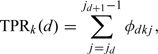
Like the definition in the situation of 2 disease classes, we could obtain true-positive rates (TPRs) and false-positive rates (FPRs) of each status class and each for doctor under a given cut point sequence as follows:

and

(2.1)

which could be used to evaluate the diagnostic accuracy of different doctors.

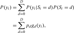
We define φ_dkj = P(T_k = j|S = d) for every d = 0,1,…,D,k = 1,2,…,K, and j = 0,1,…,J, subjecting to the normalizing conditions ∑_{j = 0}^Jφ_dkj = 1 for every d = 0,1,…,D and k = 1,2,…,K. Then we can write the TPRs and FPRs as follows:

and

(2.2)

Therefore, to evaluate the diagnostic accuracy of different doctors, we need to estimate φ_dkj. Since we do not know the true symptom status S and its distribution, we propose an extension of the nonparametric method by Zhou and others (2005) in the 2-class situation without a gold standard to a D-class situation like ours here.

First, we assume that given the true symptom status, the diagnoses of different doctors are independent with each other. This assumption does not usually hold when considering a disease since doctors may have learned the same theory and trained to look for certain symptoms. However, as for a specific symptom, this assumption may be reasonable because doctors do not look for further surrogates but just give their own opinions on whether this symptom is mild or severe. Take a symptom, extremities cold, in our real data study as an example. Doctors examine patient' hand and foot, then give their judgment on whether the patient's symptom is normal, slight cold, or frozen according to their own choice of “cut points.” Therefore, conditional on the true symptom status, doctors' decision on a symptom could be independent. We will give more explanation on feasibility of this assumption before we apply our method to a real data set in Section 4.

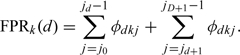
Let y_ikj be a binary variable such that y_ikj = 1 if the diagnostic result of the kth doctor is j for the ith patient and y_ikj = 0 otherwise, where i = 1,2,…,N,k = 1,2,…,K, and j = 0,1,…,J. Then we can construct a K×(J+1) dimensional vector of binary variables y_i, such that y_i = (y_i10,…,y_i1j,…,y_ik0,…,y_ikj), which reflect the diagnostic results of the ith patient. Let S_i denote the true symptom status. Under the assumption that the diagnostic results of different doctors are conditionally independent given the true symptom status, we could write the conditional probability of having ith patient's diagnostic result y_i given their symptom statuses S_i as follows:

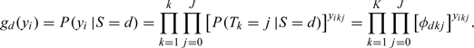The likelihood contributed by the ith patient has a mixture form of

where p_d = P(S_i = d) for d = 0,1,…,D are the prevalence rates of the symptom statuses. This is a finite mixture model with D components. The finite-sample and asympotic properties of the estimators are described by Hall and Zhou (2003).

Hence, the joint log likelihood of the observed data of all N patients, y = (y₁,…,y_N)^′, is given by

where p = (p₀,…,p_d),φ = (φ₀,…,φ_d), and φ_d = (φ_d10,…,φ_d1J,…,φ_dk0,…,φ_dkJ).

To find the ML estimates for p = (p₀,…,p_d), and φ = (φ₀,…,φ_d), subjecting to the normalizing conditions ∑_{j = 0}^Jφ_dkj = 1 for every d = 0,1,…,D and k = 1,2,…,K, we employ the expectation–maximization (EM) algorithm by treating S as missing data. Here, our complete data are (y,S), and the complete-data log likelihood is as follows:

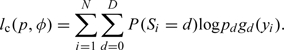We let p^(t) = (p₀^(t),…,p_d^(t)) and φ^(t) = (φ₀^(t),…,φ_d^(t)) indicate the estimates of p and φ after the tth iteration of the EM algorithm. The conditional expectation of complete-data log likelihood given the observed data y and the current parameter estimates p = p^(t) and φ = φ^(t), computed in the tth step, is given as follows:

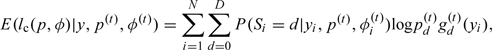where

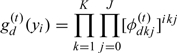and

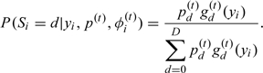In M-step, we find the updated estimates of parameters by maximizing the conditional expectation of complete-data log likelihood, computed in E-step, with respect to p and φ, which result in the following explicit expressions:

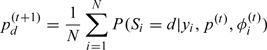and

Therefore, according to the theory of EM algorithm, the convergent values from the above EM algorithm give us MLEs of the parameters, denoted by . However, as mentioned by Zhou and others (2005), these ML estimates may be sensitive to the selection of the initial parameter estimates, and the recommendations are to avoid taking equal φ_0kj = φ_1kj = ⋯ = φ_Dkj for all k and j as initial values and to try a set of reasonable initial parameter estimates and compare the local log-likelihood maxima obtained.

2.2. Indicator and graphical representation of the accuracy in D-class diagnostic task

Although the parameters φ_dkj = P(T_k = j|S = d), in the previous section, could give us the information needed in evaluating the diagnostic accuracy of different doctors, it may be difficult to summarize these conditional probabilities into an overall measure of doctors' diagnostic accuracy in detecting the symptom when the true symptom status is a high-dimensional class. In dichotomous true symptom tasks, ROC analysis is used to depict diagnostic accuracy by plotting the TPR ( = test sensitivity) as a function of the FPR ( = [1 − test specificity]) as the decision threshold is moved through its range of possible cut-points, and the area under an ROC curve (AUC) could be used to summarize doctors' overall accuracy. As for a trichotomous true symptom task, Mossman (1999) presented an ROC surface on 3D coordinates and its volume as an overall measure of accuracy. However, this method has a visual problem when the true symptom has a high dimension. Here, we extend his concept to an n-dimensional true symptom status.

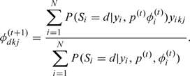
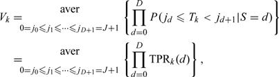
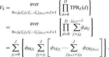
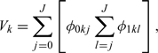
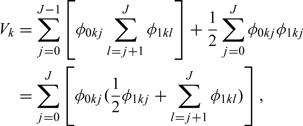
The TPRs and FPRs of each status class and each doctor under a given cut-point sequence are given by (2.1) in the previous section. Here, we define the overall accuracy V as the averaged probability of correctly diagnosing a symptom status as the true status under a random selected sequence of cut-points {j₀ = 0,j₁,…,j_{D + 1} = J + 1},(j_d ≤ j_{d + 1} for every d = 0,…,D), i.e. the overall accuracy of the kth doctor is given by

where “aver” is referred as an average operator.

Using (2.2),we can rewrite the above equation as follows:

(2.3)

We notice that this is an equivalent concept as AUC in 2-class diagnostic task and volume under the ROC surface (VUS) in 3-way ROC: if we depict the points (TPR_k(1),…,TPR_k(D)) in a D-dimension coordinates, where the projection on the ith axis is TPR_k(i), the volume under the terrace-shaped hypersurface generated by these points is (2.3). The proof for the equivalence of the overall accuracy measure V, and the AUC in the case of a 2D disease status can be found in Section A of the supplementary material available at Biostatistics online. It is not hard to understand this equivalence. Recall in the case of 2D disease status, the AUC is the average of TPRs over all possible specificities, i.e. the AUC can be interpreted as the probability of correct ranking of test results, one being randomly chosen from the diseased population and the other being randomly chosen from the nondiseased population. Mossman (1999) extended this concept to his 3-way ROC surface, where the VUS was equal to the probability that a triplet randomly chosen from 3 different groups will be correctly ranked by the decision maker. In our case, rather than simply defining the TPR as the probability that a doctor would not understate or overstate the symptom statuses of the patient, which equal to the probability that the diagnostic result is higher or lower than a cut-point, we define TPRs as the probability that the diagnostic result is between 2 cut-point. Thus, the average of TPR could be interpreted as the probability of correct ranking all test results, and V_k is an extended VUS in high dimension and could reflect the diagnostic accuracy of the kth doctor.

If doctors' responses are continuous, P(T_k = t|S = d) are smooth functions f_kd(t), and (2.3) could be written as follows:

(2.4)

where f_k is the function of a smooth hypersurface of the diagnostic result in D-dimension.

In a special case of the 2-class diagnostic task, if the diagnosis probabilities P(T_k = j|S = d) are discrete, the overall accuracy indicator, defined by (2.3) is reduced to the following expression:

which is equal to the AUC when we use terrace-shaped lines to connect the points. If we use inclined lines rather than terrace-shaped lines to connect the points, which means P(T_k = t|S = d) are linear functions, we will use (2.4) to get the overall accuracy indicator as

which is equal to the AUC under the trapezoidal rule.

In addition, the result for 3-class diagnostic task with inclined planes connecting the points is given as follows:

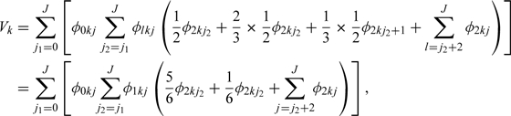which is the VUS of the 3-way ROC surface.

Also, when evaluating the diagnostic accuracy of different doctors, we should notice that the accuracy indicator defined above is 1/D! for a random guess rather than 1/2 as in dichotomous cases.

Although the overall accuracy defined above is equal to the volume under the D-dimension ROC surface as we pointed out, it is difficult to depict this high-dimensional ROC surface in a visible graph. Inspired by Ferri and others (2003), we propose 2 arachnoid graphs to show a visual result that can present the diagnostic ability of each doctor.

The graph of accuracy represents the probabilities of correct diagnosis. It contains D radials as axes, representing D symptom statuses, and the scale on each of the radials denotes the possibility of correct diagnosis regarding to this symptom status. The graph of inaccuracy reflects the probabilities of incorrect conclusion with different types of errors. Specifically, it contains D×(D − 1) radials labeled as d→j. The points on axis d→j indicate the probability that the diagnostic result T is j when the true symptom status S is d, i.e. the values of φ_dkj = P(T_k = j|S = d), different colors represent different doctors. Consequently, a better doctor tends to occupy a larger area in the graph of accuracy and a smaller area in the graph of inaccuracy, which could help us to visualize the diagnostic abilities of different doctors. An example, when K = 5 and D = J = 3, is shown in Figure 1. The axes in the left arachnoid graph are only those when d equals to j, which show the probability of correct diagnosis, and the right arachnoid graph shows the probability of incorrect diagnosis.

Fig. 1.

Arachnoid graphs presenting doctors' diagnostic abilities based on TPRs and FPRs.

There are other available methods to present the diagnostic capabilities of the doctors. For example, if it is important to know the over/underestimated symptom status level, the classification profile (CP) can be used, which is based on the probabilities P(T = i|S = j) and an index k defined by k = i − j. Thus, k is zero for the probability of accurate diagnosis, is negative for the probabilities of underestimation and is positive for overestimation. An example with D = J = 3 is shown in Figure 2. The shape of the CP graphically reflects overall diagnosis performance. A CP, which has a relatively high and narrow peak at k = 0, corresponds to a doctor who classifies symptom status accurately, and a CP, which is most flat, is from a bad doctor. A plot skewed to the left of the zero vertical line indicates a doctor who tends to underestimate the symptom status level, while a plot skewed to the right tends to overestimate the symptom status level.

Fig. 2.

Sketch map of the CP.

3. SIMULATION STUDY

In this section, we carried out simulation studies under different levels of the diagnostic performance of doctors as well as different prevalence rates in the different classes of a symptom to assess the performance of the nonparametric method and the overall diagnostic accuracy described in the previous section. For simplicity, we chose K = 5 and D = J = 4 as in our real data set. Since in practice, it is difficult to collect the data in which one patient is diagnosed by many doctors, the total number of patients N could not be very large. In our simulation, we chose the number of patients as 20 and 40. We considered 3 different prevalence rates for each sample size. The first scenario assumed equal portions for patients with different symptom severity. The second one assumed that more patients were of heavier symptom status. And the last assumption considered U-shaped prevalence rates, where most patients are in the asymptomatic and severe groups, while less patients are in the 2 groups with mild or moderate symptom status.

We simulated 5000 data sets under each setting. We then implemented the proposed method to obtain the parameter estimates. As for the choice of initial values, we avoided equal φ_0kj = φ_1kj = ⋯ = φ_Dkj for all k and j as mentioned previously. To avoid reaching a local maximum, we used a number of initial values, then compared the local log-likelihood maxima obtained for each of the chosen initial values before deriving the global ML estimates. In addition, we also used the initial values given by experts of TCM and the results were the same. We focus on assessing the bias and mean squared error (MSE) of the estimates of the diagnostic accuracy indicators under different settings. The results were shown in Table 1. To help better evaluate the performance of all estimates, the biases and MSEs of all φ_dkj with d = 0,1,…,3, k = 1,2,…,5, and j = 0,1,…,3 were also summarized in the last 3 columns of Table 1.

Table 1.

Results from 5000 simulations with D = 3, K = 5, and J = 3 under various prevalence rates and parameter settings

Patient number N = 20
True prevalence rates	Statistics	V1	V2	V3	V4	V5	φdkj*
	True values	0.356	0.408	0.505	0.606	0.703	max	min	mean
p0 = 0.25, p1 = 0.25	Bias	– 0.014	– 0.014	– 0.024	– 0.026	– 0.035	0.046	0.000	0.017
p2 = 0.25, p3 = 0.25	MSE	0.045	0.050	0.057	0.069	0.059	0.123	0.003	0.046
p0 = 0.10, p1 = 0.20	Bias	– 0.016	– 0.018	– 0.024	– 0.019	– 0.03	0.098	0.000	0.024
p2 = 0.30, p3 = 0.40	MSE	0.050	0.062	0.064	0.06	0.078	0.168	0.006	0.051
p0 = 0.25, p1 = 0.10	Bias	– 0.031	– 0.021	– 0.015	– 0.023	– 0.058	0.357	0.001	0.042
p2 = 0.15, p3 = 0.50	MSE	0.050	0.058	0.064	0.065	0.087	0.199	0.003	0.066
Patient number N = 40
p0 = 0.25, p1 = 0.25	Bias	– 0.014	– 0.008	– 0.008	– 0.003	– 0.030	0.033	0.000	0.008
p2 = 0.25, p3 = 0.25	MSE	0.019	0.022	0.024	0.026	0.029	0.045	0.004	0.023
p0 = 0.10, p1 = 0.20	Bias	– 0.014	– 0.013	– 0.013	– 0.010	– 0.039	0.042	0.000	0.011
p2 = 0.30, p3 = 0.40	MSE	0.024	0.028	0.031	0.030	0.039	0.077	0.003	0.028
p0 = 0.25, p1 = 0.10	Bias	– 0.015	– 0.014	– 0.015	– 0.016	– 0.044	0.045	0.001	0.012
p2 = 0.15, p3 = 0.50	MSE	0.021	0.024	0.028	0.028	0.036	0.073	0.003	0.028

^*Results for all φ_dkj with d = 0, 1, …, 3, k = 1, 2, …, 5, and j = 0, 1, …, 3.

From the results, we can see that the proposed method yields ML estimates for the overall diagnostic accuracy with small biases and MSEs regardless of the true diagnostic performance of doctors and true prevalence rates of the statuses of a symptom. The summary result of all φ_djk also support our method. We can see that even the maximum bias and MSE are not very large. In general, the results were slightly better when the prevalence rates of different symptom statuses were similar. And the larger the number of patients was, the smaller were the estimated bias and MSEs of the estimates.

The conditional independence assumption is crucial in the proposed method. Although it is reasonable in our real data problem, it is helpful to evaluate the robustness of the method when this assumption is violated. Suppose except for the true symptom status, there were some doctor-level covariates R that would influent the doctors' decision. As a result, instead of conditional independence giving the true symptom status, the diagnosis results were correlated unless providing both true symptom status S and covariates R. In these simulations, we suppose doctors' decision was influenced by the covariate R via coefficient b through a probit model, where R follows a normal distribution with mean 0 and standard deviation 0.5. Specifically, P(T_ik = j|S_i = d,R_k = r) = Φ(a_dkj + br), for i = 1,…,N, d = 0,1,…,D, and k = 1,2,…,K. We chose sample size N = 34 as in our real data set and simulated 5000 data sets under the 3 prevalence scenarios as before, i.e. equal portions with p₀ = 0.25,p₁ = 0.25,p₃ = 0.25,p₄ = 0.25; increasing prevalence p₀ = 0.1,p₁ = 0.2,p₃ = 0.3,p₄ = 0.4; and U-shaped prevalence p₀ = 0.25,p₁ = 0.1,p₃ = 0.15,p₄ = 0.5. In each setting, we considered 3 different correlation level by setting b equal to 0.2, 0.5, and 1. The results on bias of the estimates were shown in Table 2, with MSEs in the parenthesis.

Table 2.

Robustness performance from 5000 simulations when D = 3, K = 5, and J = 3 and patient number N = 34. Covariate R follows normal distribution with mean 0 and standard deviation 0.5, and influent diagnosis with coefficient b

True prevalence rates	Statistics	V1	V2	V3	V4	V5	φdkj
	True values	0.356	0.408	0.505	0.606	0.703	Maximum	Minimum	Mean
p0 = 0.25,	0.2	– 0.008**	– 0.012	– 0.019	– 0.032	– 0.023	0.067	0.000	0.017
p1 = 0.25		(0.020)***	(0.020)	(0.023)	(0.026)	(0.027)	(0.040)	(0.003)	(0.021)
p2 = 0.25,	0.5	– 0.009	– 0.003	– 0.003	– 0.018	– 0.018	0.129	0.000	0.030
p3 = 0.25		(0.015)	(0.018)	(0.019)	(0.023)	(0.020)	(0.035)	(0.002)	(0.020)
	1.0	– 0.030	– 0.01	– 0.039	– 0.042	– 0.031	0.271	0.003	0.054
		(0.018)	(0.020)	(0.024)	(0.026)	(0.027)	(0.048)	(0.001)	(0.022)
p0 = 0.10,	0.2	– 0.015	– 0.023	– 0.034	– 0.047	– 0.053	0.132	0.000	0.025
p1 = 0.20		(0.026)	(0.034)	(0.037)	(0.039)	(0.052)	(0.106)	(0.002)	(0.030)
p2 = 0.30,	0.5	– 0.012	– 0.016	– 0.013	– 0.027	– 0.011	0.146	0.000	0.028
p3 = 0.40		(0.016)	(0.021)	(0.026)	(0.025)	(0.025)	(0.062)	(0.001)	(0.023)
	1.0	– 0.023	– 0.020	– 0.036	– 0.038	– 0.021	0.293	0.002	0.053
		(0.015)	(0.025)	(0.032)	(0.023)	(0.026)	(0.068)	(0.001)	(0.024)
p0 = 0.25,	0.2	– 0.018	– 0.018	– 0.009	– 0.018	– 0.028	0.084	0.000	0.019
p1 = 0.10		(0.018)	(0.021)	(0.021)	(0.022)	(0.027)	(0.066)	(0.002)	(0.024)
p2 = 0.15,	0.5	– 0.019	– 0.008	– 0.019	– 0.02	– 0.03	0.151	0.000	0.036
p3 = 0.50		(0.017)	(0.018)	(0.022)	(0.021)	(0.026)	(0.074)	(0.001)	(0.026)
	1.0	– 0.038	– 0.016	– 0.026	– 0.028	– 0.051	0.236	0.000	0.062
		(0.016)	(0.022)	(0.027)	(0.026)	(0.028)	(0.096)	(0.001)	(0.029)

^*Bias ^∗∗MSE

From the results, we can see that with correlations induced by the covariates, both the biases and MSEs are larger than those when conditional independence assumption holds. However, when the influence of the covariates to the diagnosis results were not very large, i.e. when the dependence was mild, the results were still acceptable. But as we expected, when the covariates have bigger influences, the biases and MSEs were increased. This suggests that the conditional assumption is necessary for the proposed method. And it is not suitable in the situation where the diagnostic results are highly correlated even conditional on the true symptom status.

In addition, we also performed additional simulation to assess the estimators' performance on the boundary of the parameter space, i.e. some of the diagnosis probabilities φ_dkj were zero. This question was first raised by the results of the real data analysis, where some of these quantities were estimated as zero. The parameter setup in the simulation used the estimated values of these parameters from the real data study. Results were shown in Section B of the supplementary material available at Biostatistics online. The results do not suggest that the proposed method have any different performance in these settings from the settings before.

4. REAL DATA STUDY

In this section, we applied the proposed method to assess 5 doctors' diagnostic abilities concerning a certain disease based on a real TCM data set. The data were the syndrome differentiation results concerning Chills disease collected in 2005 at Xiaoyudong Village of Sichuan Province of China. Chills disease is caused by irregular dietary and life habit, hormone imbalance, and can lead to abnormal vascular contraction and expansion, decreased blood circulation function, and peripheral nerve excretion not fully discharged. Patients who suffer from Chills disease often have the following symptoms: hands and feet cold, headache or shoulder stiffness, fatigue, irritability, insomnia, and so on. Although it is relatively easy to tell whether a person has or does not has a Chills disease, more detailed information of the diagnosis on the severities of different symptoms is needed for choosing right treatments. However, diagnoses on a particular symptom are based on doctors' judgments and could vary greatly. It is important to assess the relative diagnostic accuracy of different doctors.

In this data set, 34 patients were diagnosed by 5 doctors independently. The data set contained the diagnostic results of the 5 doctors on 12 symptoms of wind-phobia, extremities cold, body cold, sniveling, abdomen pain, warmphlie, crouchingness, liking for knead, inappetence, liking mild temperature, cold-sensitiveness, and cold-phobia, which are related to the Chills disease. For convenience, we denoted the symptoms as symptom 1 to symptom 12, respectively. The diagnostic results were given by an ordinal scale, 0, 1, 2, and 3, representing the doctors' opinion that the symptom status of the patient was asymptomatic, slight, middle, or severe, respectively. The conditional independence assumption was necessary for our ML estimates, i.e. given the true symptom statuses, doctors' diagnoses on the symptoms should be independent to each other. In our case, this assumption is reasonable because doctors examined some specific symptoms which did not have further surrogates in this study. They made their own diagnoses, based on their own judgment of cut-points rather than any common principles or common variables. It was unlikely to have any common covariates that influenced their decision. Taking symptom 1, wind-phobia, as an example, each doctor gave his/her own opinion about the severity that the patient was sensitive to the wind. The doctors did not know the diagnosis results of others, and their conclusions were reached according to their own perceptions about the patients' symptoms. Thus, when the true symptom status was given, their diagnoses were most likely to be independent. Since the real statuses of the symptoms, the gold standard in our case, unknown for all patients, we use the proposed method to assess the diagnostic abilities of these 5 doctors.

First, we applied the method described in Section 2.1 to obtain the ML estimates of the parameters φ_dkj = P(T_k = j|S = d), i.e. the probability that the diagnostic result was j when the true symptom status was d. Here, D = 3, K = 5, and J = 3. The results of symptom 1 were shown as an example in Table 3. The overall diagnostic accuracies proposed in Section 2.2 were also given to provide a general evaluation of doctors' performance.

Table 3.

Parameter estimates and corresponding overall accuracies estimates in detecting symptom 1

	Doctor 1	Doctor 2	Doctor 3	Doctor 4	Doctor 5
P(T = 0|S = 0)	0.869	0.584	0.718	0.783	0.934
P(T = 1|S = 0)	0.125	0.416	0.282	0.217	0.066
P(T = 2|S = 0)	0.000	0.000	0.000	0.000	0.000
P(T = 3|S = 0)	0.006	0.000	0.000	0.000	0.000
P(T = 0|S = 1)	0.306	0.378	0.000	0.448	0.049
P(T = 1|S = 1)	0.376	0.574	0.704	0.443	0.907
P(T = 2|S = 1)	0.000	0.047	0.296	0.069	0.044
P(T = 3|S = 1)	0.317	0.000	0.000	0.040	0.000
P(T = 0|S = 2)	0.198	0.000	0.000	0.000	0.093
P(T = 1|S = 2)	0.000	0.193	0.076	0.162	0.308
P(T = 2|S = 2)	0.410	0.727	0.671	0.654	0.265
P(T = 3|S = 2)	0.392	0.079	0.253	0.184	0.334
P(T = 0|S = 3)	0.037	0.101	0.000	0.000	0.175
P(T = 1|S = 3)	0.000	0.048	0.014	0.041	0.319
P(T = 2|S = 3)	0.225	0.731	0.141	0.146	0.378
P(T = 3|S = 3)	0.739	0.121	0.845	0.813	0.128
Vk	0.550	0.650	0.906	0.786	0.389

In order to give a more clear perception of the doctors' diagnostic accuracy, we drew 2 arachnoid graphs based on Table 1 to show the accuracy and inaccuracy as discussed in Section 2.2. The pictures were reported in Figure 1. The points in the left arachnoid graph were the probabilities of correct diagnosis of the symptom and the right arachnoid graph showed the probabilities of incorrect diagnosis. In addition, we also drew a CP plot in Figure 3. From the graphs, we could see that in general, the diagnostic ability of Doctor 3 on symptom 1 was better than the other doctors, while the ability of Doctor 2 was not so good. Besides, Doctor 4 was slightly better than Doctor 1, and both Doctors 3 and 4 had better performance than Doctor 5.

Fig. 3.

CP plots of the 5 doctors.

Finally, we applied the proposed method to all of those 12 symptoms in data set and calculated the overall diagnostic accuracy given in Section 2.2. The results showed that the diagnostic accuracy of Doctor 3 was the best. Meanwhile, the performance of Doctors 2 and 5 were not so good. Doctor 4 performed slightly better than Doctor 1 but not as good as Doctor 3. Besides, although for all the symptoms, the standard deviations of diagnostic accuracy of different doctors were not very large, estimated accuracy of a doctor can vary for different symptoms. We also notice that the diagnostic accuracy was more stable for Doctors 2 and 3, and fluctuant for Doctors 1 and 4. For detailed results about the estimates of doctors' diagnostic accuracies and the standard deviations based on the standard bootstrap method, please refer to Section C of the supplementary material available at Biostatistics online.

5. DISCUSSION

In this paper, we have proposed a nonparametric ML method for estimating the accuracy of ordinal scale diagnostic tests when the gold standard on the true severity of symptom has an ordinal scale and is not available. The explicit solution at M-step makes it much easier to implement the corresponding EM algorithm. Our simulation results have shown the proposed estimators have good small bias and MSE in small sample sizes.

We use 2 arachnoid graphs and the CP plot to visually present the diagnostic ability of each doctor in distinguishing severity levels of a symptom. The graphs are easier to interpret than the series of estimators and can provide more information about diagnostic performance than the single overall accuracy measure V_k. Specifically, we can assess the inclination of underestimation or overestimation of doctors under different symptom statuses.

The proposed nonparametric method requires the conditional independence assumption. Although this assumption is reasonable in our example when considering a specific symptom, there are many other situation in which this assumption is questionable, and conditional dependence structure among different doctors should be considered. One area of further research is to develop a parametric ML method without assuming conditional independence. For example, we may use a log-linear model without higher-order interactions to relax this assumption. Or, we can consider utilizing a random-effect modeling approach, which has become very popular for correlated tests and discussed by Hadgu and Qu (1998), Qu and Hadgu (1998) with binary disease status. Thompson (2003) also discussed methods for assessing diagnostic accuracy from repeated binary screening tests.

Another extension is to deal with a symptom or disease status with a nominal scale. In our case, the symptom status has an ordinal scale from 0 to 3, denoting the severity of symptom from asymptomatic to severe. However, there are some situations in which we use discrete values to indicate different subdiseases. For example, in the diagnosis of cancer, a doctor may be interested in determining whether it is a lung cancer, colon cancer, or other types. Our definition of TPR, FPR, and the overall accuracy indicator did not include information of severity, rather, the TPR only includes the situations where the diagnosis results agree with the true symptom status while both underdiagnosis and overdiagnosis belong to FPR. This essentially gives equal weight to all type of errors, although one might consider giving different weight when some errors are known to be more harmful. With our definitions, the approach could be easily extended to a nominal scale once the diagnosis strategy for the nominal status are determined. However, without ordering, this kind of diagnosis problem is much harder. Nakas and Alonzo (2007) gave a discussion when the disease classes have an umbrella ordering. They essentially viewed this problem as a combination of the 2 possible sequential. A similar method of considering a nominal scale as a combination of all possible ordering might be one approach to address diagnosis problem with a nominal scale.

SUPPLEMENTARY MATERIAL

Supplementary material is available at http://biostatistics.oxfordjournals.org.

FUNDING

National Natural Science Foundation of China (30728019); National Institutes of Health (R01EB005829).

References

- Chi YY, Zhou XH. ROC surfaces in the presence of Verification Bias. Journal of Royal Statistical Association, Series C, Applied Statistics. 2010;57:1–23. [Google Scholar]
- Fawcett T. Proceedings IEEE International Conference on Data Mining. San Jose, CA: IEEE Computer Society; 2001. Using rule sets to maximize ROC performance. Print ISBN: 0-7695-1119-8, pp. 131–138. [Google Scholar]
- Feng Y, Wu Z, Zhou X, Zhou Z, Fan W. Methodological review: knowledge discovery in traditional Chinese medicine: state of the art and perspectives. Arificial Intelligence in Medicine. 2006;38:219–236. doi: 10.1016/j.artmed.2006.07.005. [DOI] [PubMed] [Google Scholar]
- Ferri C, Hernandez-Orallo J, Salido MA. Volume under the ROC Surface for Multi-Class Problems. 14th European Conference on Machine Learning, ECML'03. LNAI Springer. 2003;Vol 2837:108–120. [Google Scholar]
- Hadgu A, Qu Y. A biomedical application of latent class models with random effects. Applied Statistics. 1998;47:603–616. [Google Scholar]
- Hall P, Zhou XH. Nonparametric estimation of component distribution in a multivariate mixture. Annals of Statistics. 2003;31:201–224. [Google Scholar]
- Hand DJ, Till RJ. A simple generalisation of the area under the ROC curve for multiple class classification problems. Machine Learning. 2001;45:171–186. [Google Scholar]
- Henkelman RM, Kay I, Bronskill MJ. Receiver operator characteristic (ROC) analysis without truth. Medical Decision Making. 1990;10:24–29. doi: 10.1177/0272989X9001000105. [DOI] [PubMed] [Google Scholar]
- Hui SL, Zhou XH. Estimating the error rates of diagnostic tests without gold standards. Statistical Methods in Medical Research. 1998;7:354–370. doi: 10.1177/096228029800700404. [DOI] [PubMed] [Google Scholar]
- Kaptchuk TJ. The Web That Has No Weaver: Understanding Chinese Medicine. Chicago, IL: McGraw-Hill Professional; 2001. [Google Scholar]
- Thompson ML. Assessing the diagnostic accuracy of a sequence of tests. Biostatistics. 2003;4:341–351. doi: 10.1093/biostatistics/4.3.341. [DOI] [PubMed] [Google Scholar]
- Mossman D. Three-way ROCs. Medical Decision Making. 1999;19:78–89. doi: 10.1177/0272989X9901900110. [DOI] [PubMed] [Google Scholar]
- Nakas CT, Alonzo TA. ROC graphs for assessing the ability of a diagnostic marker to detect three disease classes with an umbrella ordering. Biometrics. 2007;63:603–609. doi: 10.1111/j.1541-0420.2006.00715.x. [DOI] [PubMed] [Google Scholar]
- Nakas CT, Yiannoutsos CT. Ordered multiple-class ROC analysis with continuous measurements. Statistics in Medicine. 2004;23:3437–3449. doi: 10.1002/sim.1917. [DOI] [PubMed] [Google Scholar]
- Qu Y, Hadgu A. A model for evaluating sensitivity and specificity for correlated diagnostic tests in efficacy studies with an imperfect reference test. Journal of the American Statistical Association. 1998;93:920–928. [Google Scholar]
- Zhang NL. Hierarchical latent class models for cluster analysis. Journal of Machine Learning Research. 2004;5:697–723. [Google Scholar]
- Zhang NL, Yuan S, Tao C, Wang Y. Hierarchical latent class models and Statistical Foundation for Traditional Chinese Medicine. Artificial Intelligence in Medicine. 2007;4594:139–143. [Google Scholar]
- Zhang NL, Yuan S, Tao C, Wang Y. Latent tree models and diagnosis in traditional Chinese medicine. Arificial Intelligence in Medicine Archive. 2008;42:229–245. doi: 10.1016/j.artmed.2007.10.004. [DOI] [PubMed] [Google Scholar]
- Zhou XH, Castelluccio P, Zhou C. Nonparametric estimation of ROC curves in the absence of a gold standard. Biometrics. 2005;61:600–609. doi: 10.1111/j.1541-0420.2005.00324.x. [DOI] [PubMed] [Google Scholar]
Associated Data
This section collects any data citations, data availability statements, or supplementary materials included in this article.