A Min-Max Combination of Biomarkers to Improve Diagnostic Accuracy

Abstract

Diagnostic accuracy can be improved considerably by combining multiple biomarkers. Although the likelihood ratio provides optimal solution to combination of biomarkers, the method is sensitive to distributional assumptions which are often difficult to justify. Alternatively simple linear combinations can be considered whose empirical solution may encounter extensive computation when the number of biomarkers is relatively large. Moreover, the optimal linear combinations derived under multivariate normality may suffer substantial loss of efficiency if the distributions are apart from normality. In this paper we propose a new approach that linearly combines the minimum and maximum values of the biomarkers. Such combination only involves searching for a single combination coefficient that maximizes the area under the receiver operating characteristic (ROC) curves and is thus computation-effective. Simulation results show that the min-max combination may yield larger partial or full area under the ROC curves and is more robust against distributional assumptions. The methods are illustrated using the growth-related hormones data from the Growth and Maturation in Children with Autism or Autistic Spectrum Disorder (ASD) Study (Autism/ASD Study).

1. Introduction

Powerful biomarkers have become and will continue to be important tools in diagnosis, clinical delivery and research. In the area of diagnostic medicine, a biomarker is often used as a diagnosis tool to identify subjects with a disease, or at high risk of developing the disease. For example, prostate-specific antigen is used for diagnosis of prostate cancer, and high cholesterol levels are used as indicator of coronary and vascular disease. However, even the most well known and commonly used biomarkers are not 100% accurate and may incur considerable classification errors which will have serious implications on patients. It is therefore of great interest to utilize multiple biomarkers to increase accuracy so that these diagnostic tests will become part of standard of care.

For a biomarker whose values are measured on a continuous scale, its diagnostic performance in identifying diseased subjects is usually assessed via receiver operating characteristic (ROC) curves. Assuming that subjects with higher levels of the biomarker are more likely to develop the disease, a subject is classified as diseased (non-diseased) if the biomarker level is above (below) a certain threshold. Corresponding to this threshold, the biomarker’s sensitivity is the probability that a diseased subject is correctly identified, and its specificity is the probability that a non-diseased subject is correctly classified. The ROC curve of the biomarker is then a plot of its sensitivity versus one minus its specificity for all possible values of the threshold. The area and partial area under the ROC curve are popular measures of the performance of a biomarker, with larger value of the area being the better [1]. There are many reasons for the popularity of the ROC curve. It presents the benefits versus costs of screening with the biomarker. It also provides a scale where biomarkers can be meaningfully compared while original scales of measurements are often not comparable.

A number of authors have considered the problem of combining biomarkers to improve diagnostic accuracy by maximizing the area under the ROC curves. When the levels of the biomarkers in the diseased and non-diseased population both follow multivariate normal distributions, Su and Liu [2] derived the optimal linear combinations that yield largest area under the ROC curves. To date, optimal linear combinations have remained yet to be found if biomarkers follow non-normal distributions. Although Su and Liu’s [2] optimal linear combinations can be used when data are not normally distributed, they may suffer from loss of efficiency. Pepe and Thompson [3] proposed to obtain an empirical solution of the optimal linear combinations that maximize the Mann-Whitney statistic, an empirical estimate of the ROC area. This procedure is distribution-free and thus robust against distributional assumptions. However, it may become less efficient than Su and Liu’s [2] linear combination if data are normally distributed. Moreover, when the number of biomarkers is relatively larger, this empirical optimization process can be quite computationally extensive.

Green and Swets [4] and Pepe, Cai and Longton [5] noticed that if the disease status and the biomarkers’ levels satisfy a generalized linear model, then the regression coefficients are the optimal linear combinations that maximize the area under the ROC curves. Recognizing the optimality of the fundamental Neyman-Pearson lemma [6] in hypothesis testing, Baker [7,8], Eguchi and Copas [9], and Pepe, Cai and Longton [5] pointed out that the likelihood ratio provides the globally optimal combination, that is, at any given specificity, the likelihood ratio possesses the largest sensitivity among all combinations. Thus, the likelihood ratio also yields the largest ROC area. Like Su and Liu’s [2] combinations, these methods are optimal only if the (conditional) joint distribution function of the biomarkers given the disease status is correctly specified. Their performance can be substantially adversely affected if the true joint distribution functions depart considerably from the specified ones under which the combination is derived.

In this paper, we consider linear combinations of the minimum and maximum biomarkers’ levels, hereafter referred to as min-max combinations. We show in the next section that the maximum (minimum) of the biomarkers’ levels yields larger sensitivity (specificity) than any individual biomarker. Therefore a compromise between the maximum and the minimum, such as a proper linear combination of the two, is expected to perform well in certain situations. We derive the empirical optimal linear combination that maximizes the Mann-Whitney statistic, that is, the empirical area under the ROC curve. The proposed min-max procedure is nonparametric in nature and thus is robust against misspecified distributions. Furthermore, compared to the existing empirical linear combination approach, the min-max procedure involves the optimization of a single parameter, and thus numerically is more tractable. Diagnostic accuracy of the optimal min-max combination is investigated via simulation and real data examples, in comparison with other combination methods. For the settings considered, numerical results demonstrate that the min-max combination outperforms the others, for at least a plausible range of specificity.

2. Combination of Biomarkers

Consider k biomarkers whose levels are denoted by a vector M = (M₁, … , M_k). Conditioning on the disease status D, binary with 1 being diseased and 0 otherwise, the biomarkers’s levels are denoted by X = (X₁, … , X_k) for a non-diseased subject (D = 0) and by Y = (Y₁, … , Y_k) for a diseased subject (D = 1), with density function f = f(x₁, … , x_k) and g = g(y₁, … , y_k), respectively. The corresponding marginal density function is denoted by f_i and g_i for the ith biomarker. The corresponding distribution functions are denoted by F, G, F_i and G_i, respectively. According to Bamber [10], the area under the ROC curve of the ith biomarker is given by

$$A_i=\mathit{Pr}\{Y_i-X_i>0\}.$$ (1)

By combination of the k biomarkers we mean a real-valued function of the marker levels, h = h(M), mapping from the k-dimensional Euclidean space R^k onto the real line R¹. The area under the ROC curve of this combination is

$$A=\mathit{Pr}\left\{h\right(\mathbf{X})>h(\mathbf{Y}\left)\right\}.$$

When the distributions F and G can be correctly specified, the likelihood ratio function

$$\mathrm{LR}\left(\mathbf{M}\right)=\frac{g\left(\mathbf{M}\right)}{f\left(\mathbf{M}\right)}$$ (2)

yields an ROC curve that is above the ROC curves of any other combinations. Therefore LR(M) also has the largest area among all combinations.

In addition to its dependence on correct specification of distributions, the likelihood ratio combination can be quite complicated and hard to interpret to the medical investigators. A simple alternative is to use a linear combination,

$$l\left(\mathbf{M}\right)={\lambda }_1{M}_1+\dots {\lambda }_k{M}_k,$$ (3)

that may have a more meaningful practical interpretation. However, except for normal distributions, it is not clear whether an optimal solution for λ = (λ₁, … , λ_k) exists, and even if it does, whether the solution can be found, although one can always search for optimal empirical solution using the observed biomarkers’ levels.

Note that the linear combination λ yields an ROC curve with area

$$A\left(\lambda \right)=\mathit{Pr}\left\{{\lambda }_1\right(Y_1-X_1)+\cdots +{\lambda }_k(Y_k-X_k)>0\}.$$ (4)

Assuming that the biomarkers’ values follow multivariate normal distributions, with X ~ N(μ_X, ∑_X) for non-diseased subjects and with Y ~ N(μ_Y , ∑_Y) for diseased subjects, Su and Liu [2] derived the best linear combination (that maximizes the area under the ROC curves) with λ_i equal to, apart from a constant scalar, the ith component of

$${({\Sigma }_X+{\Sigma }_Y)}^{-1}({\mu }_Y-{\mu }_X).$$

If the two normal distributions have a common variance-covariance matrix, that is, ∑_X = ∑_Y , then Su and Liu’s [2] linear combination is identical to the likelihood ratio combination.

We now consider the min-max combination of the biomarkers. Let

$$M_{\mathit{max}}=\underset{1\le i\le k}{\max }{M}_i,M_{\mathit{min}}=\underset{1\le i\le k}{\min }{M}_i$$ (5)

be respectively the maximum and minimum value of the k biomarkers. Then the “new” marker M_max has larger sensitivity and smaller specificity for any given threshold than any individual biomarker, and the “new” marker M_min has smaller sensitivity and larger specificity for any given threshold than any individual biomarker. To see this, let X_max, X_min, Y_max and Y_min be similarly defined for each disease status. Then for sensitivity at a cut-point c we have

$$\mathit{Pr}\{Y_{\mathit{max}}>c\}=1-\mathit{Pr}\{Y_{\mathit{max}}\le c\}=1-\mathit{Pr}\{Y_j\le c,1\le j\le k\}\ge 1-\mathit{Pr}\{Y_i\le c\}=\mathit{Pr}\{Y_i>c\}$$

and

$$\mathit{Pr}\{Y_{\mathit{min}}>c\}=\mathit{Pr}\{Y_j>c,1\le j\le k\}\le \mathit{Pr}\{Y_i>c\}$$

for all 1 ≤ i ≤ k.

For specificity we have

$$\mathit{Pr}\{X_{\mathit{max}}\le c\}=\mathit{Pr}\{X_j\le c,1\le j\le k\}\le \mathit{Pr}\{X_i\le c\}$$

and

$$\mathit{Pr}\{X_{\mathit{min}}\le c\}=1-\mathit{Pr}\{X_{\mathit{min}}>c\}=1-\mathit{Pr}\{X_j>c,1\le j\le k\}\ge 1-\mathit{Pr}\{X_i>c\}=\mathit{Pr}\{X_i\le c\}$$

for all 1 ≤ i ≤ k.

These results indicate that M_max (M_min) is a plausible combination if sensitivity (specificity) is the primary concern, which, of course, is rarely the case. If our interest is to maximize the area or partial area under the ROC curves or to improve sensitivity over a range of specificity, then a compromise between M_max and M_min is expected to perform well, especially when distributional assumptions are difficult to justify. In the present paper we confine our attention to linear combinations of M_max and M_min, that is, combinations of the form M_λ = M_max + λM_min. The area under the ROC curve is given by

$$A\left(\lambda \right)=\mathit{Pr}\left\{\right(Y_{\mathit{max}}-X_{\mathit{max}})+\lambda (Y_{\mathit{min}}-X_{\mathit{min}})>0\}.$$ (6)

The optimal min-max combination is given by λ_opt that maximizes the area, that is,

$$A\left({\lambda }_{\mathit{opt}}\right)=\underset{\lambda }{\max }\mathit{Pr}\left\{\right(Y_{\mathit{max}}-X_{\mathit{max}})+\lambda (Y_{\mathit{min}}-X_{\mathit{min}})>0\}.$$ (7)

3. Estimation of Optimal Combinations

Optimal combinations of biomarkers usually depend on the distribution functions which are fully unspecified or involve several unknown parameters. A case-control study design can be employed to estimate these combinations. Let

$${\mathbf{X}}_i=(X_{1i},X_{2i},\dots ,X_{ki}),i=1,2,\dots ,n,$$

be the observed values of the biomarkers from a random sample of size n in the non-diseased population, and

$${\mathbf{Y}}_j=(Y_{1j},Y_{2j},\dots ,Y_{kj}),j=1,2,\dots ,m,$$

be the observed values of the biomarkers from a random sample of size m in the diseased population. If F and G are assumed to have known function forms apart from a few unknown parameters, then these parameters can be estimated by the corresponding maximum likelihood estimates obtained from the data. Replacing these parameters by their maximum likelihood estimates in the likelihood ratio function (2) then yields an estimate of the likelihood ratio combination.

If F and G are assumed to be of multivariate normal, then the mean vectors μ_X and μ_Y and the variance-covariance matrices ∑_X and ∑_Y can be estimated by the corresponding sample mean vectors and sample variance-covariance matrices. These estimates then yield an estimate of the likelihood ratio combination and Su and Liu’s [2] optimal linear combination.

Without assuming any parametric forms for the distributions, the optimal linear combination can be estimated by maximizing the Mann-Whitney statistic:

$$W\left(\lambda \right)=\frac{1}{mn}\sum _{i=1}^n\sum _{j=1}^{m}I({\lambda }_1{Y}_{1j}+\cdots +{\lambda }_k{Y}_{kj}>{\lambda }_1{X}_{1i}+\cdots +{\lambda }_k{X}_{ki}),$$ (8)

the empirical estimate of the area under the ROC curve of the combination λ. Here I(·) stands for the indicator function.

Similarly the empirical optimal min-max combination can be derived by maximizing the corresponding Mann-Whitney statistic:

$$W\left(\lambda \right)=\frac{1}{mn}\sum _{i=1}^n\sum _{j=1}^{m}I(Y_{j,\mathit{max}}+\lambda Y_{j,\mathit{min}}>X_{i,\mathit{max}}+\lambda X_{i,\mathit{min}}),$$ (9)

where for the ith non-diseased subject

$$X_{i,\mathit{max}}=\underset{1\le l\le k}{\max }{X}_{li},X_{i,\mathit{min}}=\underset{1\le l\le k}{\min }{X}_{li};$$

and for the jth diseased subject

$$Y_{j,\mathit{max}}=\underset{1\le l\le k}{\max }{Y}_{lj},Y_{j,\mathit{min}}=\underset{1\le l\le k}{\min }{Y}_{lj}.$$

The values of λs can be found numerically using the built-in function optim in the R software (free download at http://www.r-project.org/). The function provides general-purpose optimization based on Nelder-Mead, quasi-Newton and conjugate-gradient algorithms, and is widely used to solve various optimization problems such as finding the maximum likelihood estimates.

4. Simulations

It appears to be difficult to analytically compare the performance of the aforementioned combination methods because such a comparison involves the joint distribution of the maximum and minimum of correlated random variables, which is quite complicated even when the variables are jointly normally distributed. Instead we rely on simulations to make comparison among the ROC curves resulted from the combinations under investigation.

We consider four settings of the joint distributions of five biomarkers (k = 5) and estimated the ROC curves and their areas of the combinations for each setting. For each setting, 50,000 observations were generated from the underlying distributions that were used to estimate the ROC curves and their areas. We compare the min-max combination with Su and Liu’s [2] normal linear combination and the empirical linear combination. The combination parameter λ for min-max and empirical linear combinations were derived by maximizing the corresponding Mann-Whitney statistic. The normal linear combination were obtained from the sample mean vectors and sample variance-covariance matrices.

4.1. Multivariate normal distributions with equal variance-covariance

We first considered two multivariate normal distributions with different mean vectors and equal variance-covariance matrices given by μ_X = 0 and

$${\mu }_Y=\left(\begin{array}{c}\hfill 0.5\hfill \\ \hfill 0.6\hfill \\ \hfill 0.7\hfill \\ \hfill 0.8\hfill \\ \hfill 1.0\hfill \end{array}\right),{\Sigma }_X={\Sigma }_Y=\left(\begin{array}{ccccc}\hfill 1.0\hfill & \hfill 0.5\hfill & \hfill 0.5\hfill & \hfill 0.5\hfill & \hfill 0.5\hfill \\ \hfill 0.5\hfill & \hfill 1.0\hfill & \hfill 0.5\hfill & \hfill 0.5\hfill & \hfill 0.5\hfill \\ \hfill 0.5\hfill & \hfill 0.5\hfill & \hfill 1.0\hfill & \hfill 0.5\hfill & \hfill 0.5\hfill \\ \hfill 0.5\hfill & \hfill 0.5\hfill & \hfill 0.5\hfill & \hfill 1.0\hfill & \hfill 0.5\hfill \\ \hfill 0.5\hfill & \hfill 0.5\hfill & \hfill 0.5\hfill & \hfill 0.5\hfill & \hfill 1.0\hfill \end{array}\right).$$

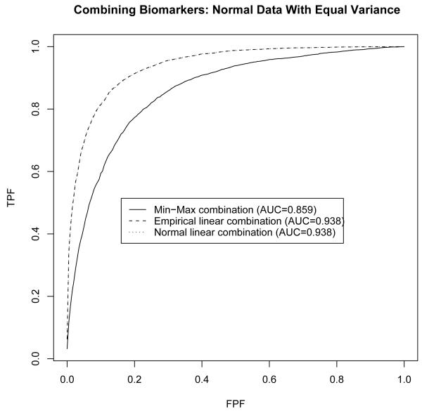
For this setting Su and Liu’s [2] linear combination is identical to the likelihood ratio combination and thus is optimal in that it yields an ROC curve which is higher than any other ROC curves. This is reflected in Figure 1 which presents the three ROC curves. In this case the min-max combination is inferior to both linear combinations which are identical. The area under the ROC curve is found to be 0.859 for min-max combination, and 0.938 for the two linear combinations.

Figure 1.

Comparison of min-max combination to linear combinations under multivariate normality with equal variances

4.2. Multivariate normal distributions with unequal variance-covariance

We next consider two multivariate normal distributions with different mean vectors and unequal variance-covariance matrices. The means and variance-covariances are the same as in Section 4.1 except that ∑_X is set to be a diagonal matrix with

$${\Sigma }_X=\mathit{diag}(1.5,1,2.5,2,3).$$

.

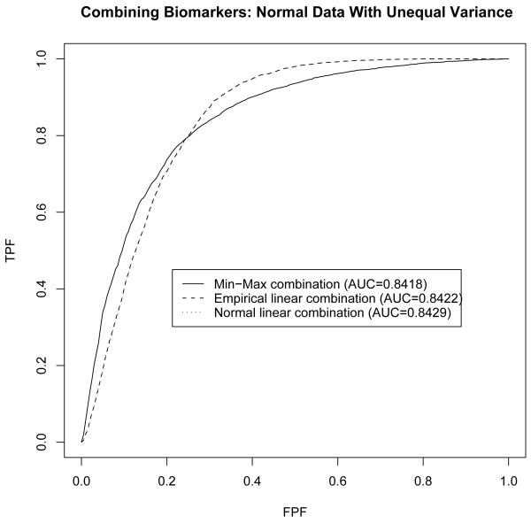
Under this setting, the likelihood ratio yields a combination that is a quadratic function of the biomarkers’ values. Su and Liu’s [2] linear combination is thus no longer the best combination, though it is among combinations with linear forms. The three ROC curves are presented in Figure 2. The areas under the three ROC curves are quite close, indicating almost identical performance when judged by the area under the ROC curve. However, a more detailed investigation reveals that the min-max yields larger sensitivity for specificity larger than 75%. This indicates that if relatively high specificity is desirable, then the min-max combination may turn out to be more appealing than linear combinations, even when levels of the biomarkers follow multivariate normal distributions with unequal variance-covariance matrices. Note that under multivariate normality assumptions, the optimal empirical linear combination is, in theory, identical to Su and Liu’s [2] optimal linear combination, as reflected in both Figure 1 and 2.

Figure 2.

Comparison of min-max combination to linear combinations under multivariate normality with unequal variances

4.3. Multivariate log-normal distributions with unequal variance-covariance

Linear combinations usually performs better when the distributions of the levels of the biomarkers are close to normal, and the variance-covariance matrices do not differ much. In this section we investigate the diagnostic accuracy of the min-max combination as compared with the linear combinations, assuming that the biomarkers’ levels follow multivariate log-normal distributions, that is, the log-transformed levels are jointly normally distributed. To this end, data from multivariate log-normal distributions are generated by exponentiating the simulated data in Section 4.2 from the multivariate normal distributions.

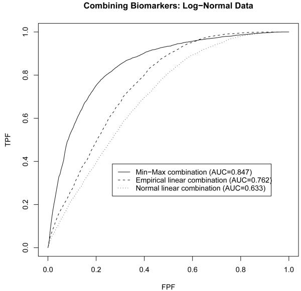
The estimated ROC curves are presented in Figure 3. The min-max combination appears to performs considerably better than the two linear combinations; it yields a relative larger area of 0.847 under the ROC curve and the ROC curve is higher than the other two over a quite large range of specificity (from about 55% to 100%). The empirical linear combination appears to be uniformly better than Su and Liu’s [2] linear combination in that it produces a higher ROC curve. This should not be surprising because Su and Liu’s [2] linear combination is optimal only under multivariate normality, and may suffer substantial loss in diagnostic accuracy if the multivariate normality assumption is violated.

Figure 3.

Comparison of min-max combination to linear combinations under multivariate log-normality

4.4. Normal-Gamma mixture

We further investigate the three combinations assuming that levels of biomarkers follow a mixed distribution of normal and gamma with equal allocation. The simulated data were obtained by adding simulated gamma data to the multivariate normal data in Section 4.2. To be specific, the biomarkers’ levels Y from the diseased population were generated by adding a gamma variate with a common shape parameter of 0.1 to the multivariate normal data. For biomarkers’ levels X in the non-diseased population, a gamma variate with shape parameter 0.1 × i was added to the ith biomarker (i = 1, 2, 3, 4, 5).

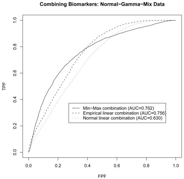
Figure 4 with the simulated ROC curves reveals trends similar to Figure 3. The min-max combination appears to be the best among the three which yields the largest area under the ROC curve. The min-max ROC curve again is higher than the other two over a quite large range of specificity (from about 75% to 100%). Su and Liu’s [2] linear combination again is the worst among the three, and appears to be uniformly inferior to the empirical linear combination, reflecting the substantial loss in accuracy with non-normal data.

Figure 4.

Comparison of min-max combination to linear combinations with multivariate normal and gamma mixture

5. An Example: Diagnosis of Autism by Combining Growth-Related Hormones

In this section we illustrate the application of the proposed min-max combination to the diagnosis of autism, a disorder of neural development characterized by impaired social interaction and communication, and by restricted and repetitive behavior.

To investigate whether children aged 4-8 years old with autism/autism spectrum disorders (ASD) are larger than matched control children and the role growth-related hormones may play, a case-control study was conducted by the Eunice Kennedy Shriver National Institute of Child Health and Human Development in 2002-2005. The study participants consisted of 81 subjects (75 boys and 6 girls) diagnosed with autism/ASD, and 80 age-matched controls (59 boys and 21 girls). Blood samples from the study participants were assayed for insulin-like growth factors (IGF-1, IGF-2), insulin-like growth factorbinding protein (IGFBP-3), and growth hormonebinding protein (GHBP), as well as for dehydroepiandrosterone (DHEA) and DHEA sulfate (DHEAS). See Mills et al. [11] for details of subject enrollment and data collection.

To serve the purpose we selected three growth hormones, IGFBP3, IGF1 and GHBP, to illustrate the performance of the min-max combination in identifying autism/ASD disease. Due to limited number of enrollments, data from the girls are excluded from the analysis. Levels of the hormones are standardized to avoid different measurement units. To ensure the optimal linear combinations to have a unique solution, the combination coefficient corresponding to IGFBP3 is set to 1. The optimal min-max combination is found to be

$$\max \{\mathrm{IGFBP}3,\mathrm{IGF}1,\mathrm{GHBP}\}+0.563\times \min \{\mathrm{IGFBP}3,\mathrm{IGF}1,\mathrm{GHBP}\}.$$

The empirical linear combination is found to be

$$\mathrm{IGFBP}3-0.05\times \mathrm{IGF}1+0.3\times \mathrm{GHBP},$$

close to the normal linear combination given by

$$\mathrm{IGFBP}3-0.039\times \mathrm{IGF}1+0.433\times \mathrm{GHBP}.$$

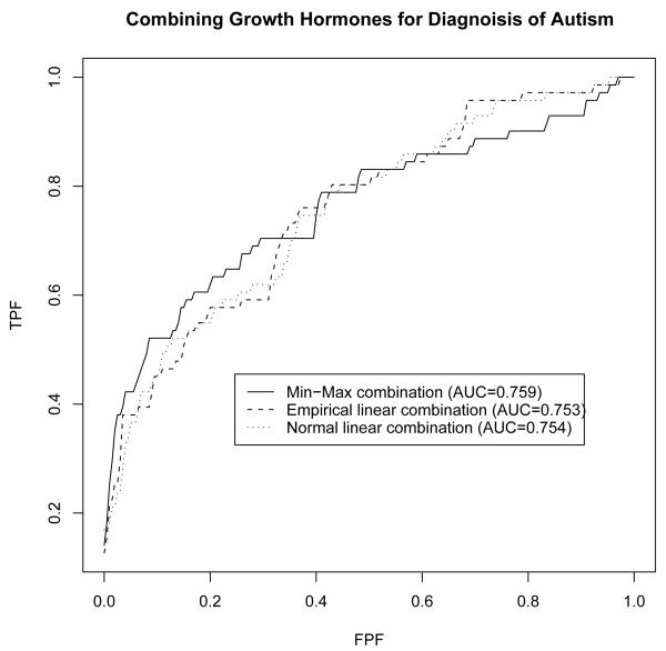
The corresponding area under the ROC curve is found to be 0.759, 0.753 and 0.754, respectively. Thus, judging by the area under the ROC curve, the min-max combination has higher diagnostic accuracy than linear combinations in identifying autism disease. Furthermore, the min-max combination yields higher specificity for sensitivity larger than 70%, a more appealing optimality property.

6. Discussion

Diagnostic accuracy, as measured by the area or partial area under the ROC curves, can be substantially improved by combining multiple biomarkers. The optimal combinations such as the likelihood ratio combination or Su and Liu’s [2] combination, however, are vulnerable to the underlying distributional assumptions, which, when violated, can yield undesirable results and will have serious implications on patients. The min-max combination proposed in the present paper, on the other hand, is nonparametric in nature. Thus, this approach is more robust against parametric models. This is demonstrated from the simulation results and the autism example. Our numerical results also showed that the min-max combination may achieve higher sensitivity over a desirable range of specificity. Similar results (data not shown) were observed from simulation on multivariate distributions that can be transformed to a multivariate normal distribution via a Box-Cox transformation, and on Ramabhadran’s [12] multivariate gamma distribution.

The min-max procedure aims at combining repeated measurements of a single biomarker over time or multiple biomarkers that are measured with the same unit. If the biomarkers are measured with different units, then the measurements need to be converted to have the same unit or to be standardized to be unit-less, as what was done in the autism/ASD example, before combining.

If, instead of sensitivity, the specificity of a biomarker is of primary concern, then the min-max combination adopts a form of specificity + λ × sensitivity. This combination is expected to be able to achieve higher specificity over a desirable range of sensitivity.

The estimated ROC curves of the combinations can be quite jagged when the sample sizes are relatively small. Smoothed ROC curves can be obtained using methods developed by Zou, Hall and Shapiro [13] and Zou and Hall [14], among others.

Future research is necessary for inference on the optimal min-max combination coefficient λ_opt, such as consistent estimation and confidence intervals. The performance of the min-max combination under other multivariate distributions is also of particular interest.

Figure 5.

Min-max combination of growth hormones IGFII, IGFBP3, IGF1, and GHBP for diagnosis of autism

References

- 1.Hanley JA, McNeil BJ. The meaning and use of the area under a receiver operating characteristic (ROC) curve. Radiology. 1982;143:29–36. doi: 10.1148/radiology.143.1.7063747. [DOI] [PubMed] [Google Scholar]
- 2.Su JQ, Liu JS. Linear combinations of multiple diagnostic markers. Journal of the American Statistical Association. 1993;88:1350–1355. [Google Scholar]
- 3.Pepe MS, Thompson ML. Combining diagnostic test results to increase accuracy. Biostatistics. 2000;1:123–140. doi: 10.1093/biostatistics/1.2.123. [DOI] [PubMed] [Google Scholar]
- 4.Green DM, Swets JA. Signal Detection Theory and Psychophysics. Wiley; New York: 1966. [Google Scholar]
- 5.Pepe MS, Cai T, Longton G. Combining predictors for classification using the area under the Receiver Operating Characteristic curve. Biometrics. 2006;62:221–229. doi: 10.1111/j.1541-0420.2005.00420.x. [DOI] [PubMed] [Google Scholar]
- 6.Neyman J, Pearson ES. On the problem of the most efficient tests of statistical hypothesis. Philosophical Transactions of the Royal Society of London, Series A. 1933;231:289–337. [Google Scholar]
- 7.Baker S. Identifying combinations of cancer markers for further study as triggers of early intervention. Biometrics. 2000;56:1082–1087. doi: 10.1111/j.0006-341x.2000.01082.x. [DOI] [PubMed] [Google Scholar]
- 8.Baker S. The central role of receiver operating characteristic (ROC) curves in evaluating tests for the early detection of cancer. Journal of the National Cancer Institute. 2003;95:511–515. doi: 10.1093/jnci/95.7.511. [DOI] [PubMed] [Google Scholar]
- 9.Eguchi S, Copas J. A class of logistic-type discriminant functions. Biometrika. 2002;89:1–22. [Google Scholar]
- 10.Bamber D. The area above the ordinal dominance graph and the area below the receiver operating characteristics graph. Journal of Mathematical Psychology. 1975;12:387–415. [Google Scholar]
- 11.Mills JL, Hediger ML, Molloy CA, Chrousos GP, Manning-Courtney P, Yu KF, Brasington M, England LJ. Elevated levels of growth-related hormones in autism and autism spectrum disorder. Clinical Endocrinology. 2007;67:230–237. doi: 10.1111/j.1365-2265.2007.02868.x. [DOI] [PubMed] [Google Scholar]
- 12.Ramabhadran VR. A multivariate gamma-type distribution. Sankhya. 1951;11:45–46. [Google Scholar]
- 13.Zou KH, Hall WJ, Shapiro DE. Smooth nonparametric receiver operating characteristic curves for continuous diagnostic tests. Statistics in Medicine. 1997;16:2143–2156. doi: 10.1002/(sici)1097-0258(19971015)16:19<2143::aid-sim655>3.0.co;2-3. [DOI] [PubMed] [Google Scholar]
- 14.Zou KH, Hall WJ. Two transformation models for estimating an ROC curve derived from continuous data. Journal of Applied Statistics. 2000;26:621–631. [Google Scholar]