Development of a Parametric Finite Element Model of the Proximal Femur using Statistical Shape and Density Modeling

Abstract

Skeletal fractures associated with bone mass loss are a major clinical problem and economic burden, and lead to significant morbidity and mortality in the aging population. Clinical image based measures of bone mass show only moderate correlative strength with bone strength. However, engineering models derived from clinical image data predict bone strength with significantly greater accuracy. Currently, image-based finite element (FE) models are time consuming to construct and are non parametric. The goal of this study was to develop a parametric proximal femur FE model based on a statistical shape and density model (SSDM) derived from clinical image data. A small number of independent SSDM parameters described the shape and bone density distribution of a set of cadaver femurs and captured the variability affecting proximal femur FE strength predictions. Finally, a 3D FE model of an ”unknown” femur was reconstructed from the SSDM with an average spatial error of 0.016 mm and an average bone density error of 0.037 g/cm³.

1. Introduction

The problem of increased risk of skeletal fractures due to bone mass loss in aging or disease is a major clinical problem leading to estimated health care costs of nearly $17 billion in the US (Burge et al. 2007, Kanis et al. 2000). Not withstanding the economic burden, non-vertebral fractures are a significant cause of morbidity and mortality in the aging population (Johnell et al. 2004, Kanis et al. 2003, Melton 2003). Thus, concerted efforts are needed to not only identify those at risk for bone fractures, but also to identify treatment strategies that can maintain the health of the skeleton with age.

Bone mineral density (BMD) measurements are widely used to determine bone strength, especially in women, and can account for up to 70% of bone strength. Attempts to directly predict fracture risk based on bone mass have been made using x-ray, ultrasound, dual energy x-ray absorptiometry (DXA), computed tomography (CT), high-resolution CT, and magnetic resonance imaging (MRI) techniques (Bauer et al. 2007, Frost et al. 2002, Genant et al. 1996, Gnudi et al. 1998, Gonnelli et al. 2005, Jiang et al. 2000, Lecouvet et al. 1997, Majumdar et al. 1999, Nicholson et al. 1997, Oden et al. 1999, Rehman et al. 2002, Ross 1997, Stewart et al. 2006, Sweeney et al. 2002, Tabensky et al. 1996, Taneichi et al. 1997). While some correlations of fracture risk with the various imaging and biochemical data have been demonstrated, they remain nonspecific and have low sensitivity (Kanis 2002a, Kanis 2002b).

Engineering models based on clinical imaging data greatly improve estimates of bone strength (Cody et al. 1999, Keyak 2001, Keyak et al. 1990, Lotz et al. 1991, Lotz et al. 1995, Testi et al. 2002). Automated finite element (FE) meshing of Quantitative CT (QCT) data has been used to predict proximal femur strength and demonstrated accuracy similar to DXA-based methods (Keyak, Meagher, Skinner and Mote 1990, Keyak et al. 1998) using linear FEA analyses, and greater accuracyusing non-linear material models (Keyak 2001). More recent applications of FE modeling to bone strength prediction incorporate smooth surface representations of the proximal femur and non-linear material models to predict failure load (Bessho et al. 2007, Bessho et al. 2004, Taddei et al. 2006) demonstrating good correlation with results from experiments.

Current applications of finite element methods are limited in that each model represents a single bone and, in order to construct a model of a similar bone from a different patient, the complete model construction procedure must be repeated; only small gains in efficiency are made when generating models of multiple bones. Furthermore, the finite element models used to date have not included parametric descriptions of bone geometry and density distribution that would allow full model definition in terms of a relatively small number of parameters. The use of parametric modeling methods would greatly reduce the time required to construct a model of an individual’s femur and, by preserving model fidelity, would not negatively impact the predictive accuracy of the model. In addition, parametric models can be used to investigate the effects of variations in specific traits on bone strength and thus could help identify those individuals at greatest risk of bone fracture.

Statistical shape modeling methods have been used to describe variability in the morphology of a population of a structure in terms of a random field representation (Cootes et al. 1994, Kaus et al. 2003, Lorenz and Krahnstöver 2000, Rueckert et al. 2003) and current applications include image segmentation, registration, object recognition, and disease diagnosis (Benameur et al. 2005, Dornaika and Ahlberg 2006, Ferrarini et al. 2006, Koikkalainen et al. 2007, Rao et al. 2006, Rueckert, Frangi and Schnabel 2003, Shan et al. 2006). Statistical shape models capture the variability of biological structures by projecting a high dimensional representation of the structure onto a lower dimensional subspace of possible shapes constructed from a population of training shapes.

The goal of this study was to implement a statistical shape modeling based method to develop a parametric finite element representation of the proximal femur shape and bone density distribution of a group of cadaveric femurs. We used this modeling methodology to identify the major components (independent combinations) of bone geometry and density that explain the majority of geometry and bone density variation within this group of cadaver femurs and we show how each independent component independently affects the predicted strength of the proximal femur. Finally, we show how this parametric modeling methodology can be used to reconstruct the three-dimensional shape and bone density distribution of a previously unseen femur.

2. Methods

2.1 Description of Femur Surfaces

A training set of seven fresh-frozen human female right femurs (69.9 ± 8.8 years old) (Anatomical Board of the State of Texas, San Antonio, TX; Anatomical Gifts Registry, Hanover, MD) were submerged in distilled water along with a density calibration standard (Mindways, Austin, TX) and scanned using a clinical helical CT scanner (Lightspeed Ultra, GE Healthcare, Chalfont St. Giles, UK). CT data was reconstructed with 0.488 × 0.488 × 1.25 mm voxels. An iterative thresholding scheme was used to extract the bones from the imaging data and triangulated surfaces were defined to describe the outer cortical boundary of each femur (Amira v. 4.0, Mercury Computing, Chelmsford, MA). One femur surface was arbitrarily chosen as the template surface and iterative closest point analyses were performed to register the remaining surfaces to the template surface (MATLAB R2006b, The Mathworks, Inc., Natick, MA).

2.2 Definition of corresponding volumetric models

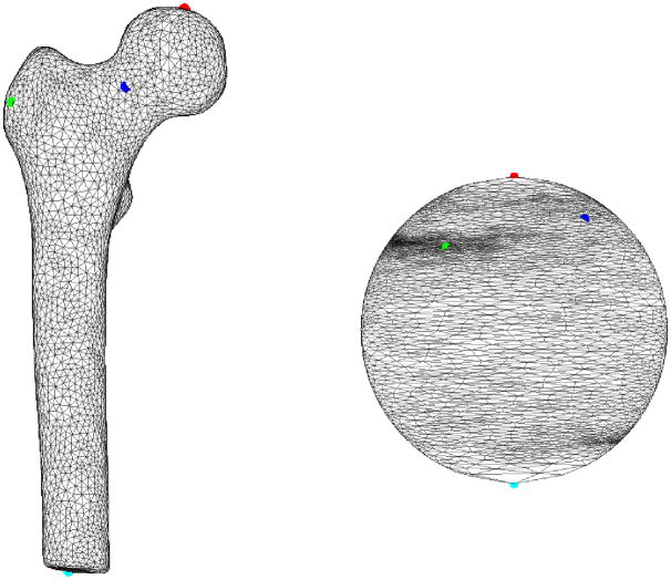
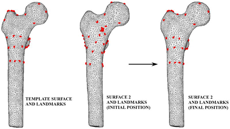
A three-dimensional (3D) finite element mesh was defined (TrueGrid, v. 2.3, XYZ Scientific Applications, Inc., Livermore, CA) and projected onto the template femur surface (Figure 1). A set of landmarks was defined by identifying the 47 specific attachment points of the computational FE mesh on the template femur surface. These landmarks were mapped onto the remaining femur surfaces using a modified closest point transform (Mauch 2000). Parametric descriptions of the femur surfaces were developed by mapping each triangulated surfaces to a unit sphere (Figure 2) (Brechbuhler et al. 1995). Point-to-point correspondence was achieved between landmarks on all femurs using a hierarchical optimization approach (Davies et al. 2002) by repositioning landmarks such that landmark variance within the training set was minimized (MATLAB) (Figure 3) (Davies, Twining, Cootes, Waterton and Taylor 2002). The FE mesh was then tied to each set of optimized landmarks and projected onto the corresponding femur surfaces to generate a total of 7 individual 3D FE meshes with mesh-to-mesh correspondence across all femurs.

Figure 1.

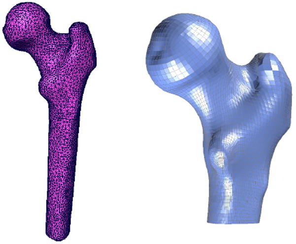
Left: Triangulated surface meshes were generated from the QCT data for each femur in the training set and hexahedral finite meshes were created for each femur using Truegrid.

Figure 2.

Each femur surface was mapped to a unit sphere, generating a parametric description of the femur surface. A set of 4 femur surface vertices are identified in both Cartesian and parametric space using red, green, blue, and cyan dots.

Figure 3.

Template landmarks (left) were mapped to the remaining femur surfaces (center). These landmarks were repositioned using a hierarchical optimization approach to minimize the spatial position variance between the template landmarks and the landmarks on the remaining femur surfaces (right).

2.3 Determination of bone mineral density distribution

QCT image intensity values corresponding to each node in each FE mesh were converted to apparent ash density using a linear relationship between known K₂HPO₄ densities in the calibration phantom and corresponding QCT image intensities (Taddei et al. 2004) along with a relationship between K₂HPO₄ density and apparent ash density (Les et al. 1994).

2.4 Statistical shape and density modeling of the femur

The finite element mesh and corresponding nodal bone density values are described by a shape and density parameter vector as

$${\mathit{p}}_{\mathit{i}}={(v_{1x},v_{1y},v_{1z},v_{1d},\dots ,v_{jx},v_{jy},v_{jz},v_{jd})}^{\text{T}}$$ (1)

where v_j(xyz) are the three dimensional coordinates of the nodes in the finite element mesh, v_jd is the corresponding bone density at that node, j=1,…, number of nodes in the finite element mesh, and i = 1…n=7 denote each femur in the training set (Davies, Twining, Cootes, Waterton and Taylor 2002). The mean finite element model of all femurs in the training set is then defined as:

$$\overline{\mathit{p}}=\frac{1}{n}\sum _{i=1}^n{\mathit{p}}_i$$ (2)

and the correlation between individual FE meshes is given by the empirical covariance matrix (Rajamani et al. 2004).

$$\mathit{S}=\frac{1}{n}\sum _{i=1}^n({\mathit{p}}_i-\overline{\mathit{p}}){({\mathit{p}}_i-\overline{\mathit{p}})}^T$$ (3)

Principal component analysis (PCA) of S results in a set of eigenvalues (λ_i) and eigenvectors (q_i) (Rueckert, Frangi and Schnabel 2003) that are the principal directions of a shape and bone density space centered at p̄. Each eigenvalue defines the variance of the finite element mesh and corresponding bone density values from the mean in the direction of the corresponding eigenvector. The proportion of the total variance described by each eigenvector is equal to its corresponding eigenvalue normalized by the total variance (sum of all eigenvalues). The finite element mesh with associated bone density for each bone in the training set is now described as a statistical shape and density model (SSDM):

$${\mathit{p}}_v=\overline{\mathit{p}}+\sum _{j=1}^m{c}_j\sqrt{{\lambda }_j}{\mathit{q}}_j$$ (4)

where p_v is a vector containing coordinates and apparent bone density value for all nodes in the FE model, m is the number of eigenvalues, λj, , and deviation from the average femur, p̄, was determined as the sum of the products of a set of scalar weighting factors, c_j, and SSDM standard deviations, $\sqrt{{\lambda }_j}$, along the q_j (eigenvector) direction (Bredbenner et al. 2007)

2.5. Parametric finite element model generation

Multiple finite element models were developed using Eq. 4 and by setting m = m_M, the number of major eigenvalues (i.e. the eigenmodes that describe greater than 75% of the total training set variability).. FE models were developed for the mean geometry and bone density distribution as well as one each investigating the effects of ±1 standard deviation (SD) for each major independent eigenmode

For each FE model, apparent ash density was determined for each element as the mean of included nodal ash densities and binned into a total of 20 apparent ash density levels. Elastic- plastic material behavior with linear hardening was assumed, and isotropic elastic and hardening moduli and ultimate stress values were determined as functions of ash density for all bone elements using empirical relationships (Keller 1994). Fall loading was simulated by fixing the distal and greater trochanter nodes in each FE model and a vertical displacement was prescribed to a flexible cup contacting the medial side of the femoral head (Figure 4). Finite element models were solved using LS-DYNA (v. 970, LSTC, Livermore, CA).

Figure 4.

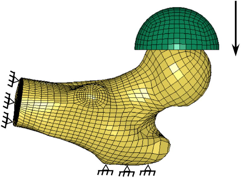
Statistical shape and density finite element model boundary conditions. The finite element model was oriented in a simulated fall position with the distal and greater trochanter nodes fully constrained. Load was applied through a rubber cup in displacement control until a total displacement of 15 mm. Load was monitored by summing the reaction forces at the greater trochanter nodes.

2.6 Investigation of the physical meaning of SSDM principal components

To relate the principal components of the SSDM to physical descriptors of bone geometry, five measures of proximal femur geometry were quantified to determine femoral neck axis length, femoral neck diameter, neck-shaft angle, femoral head diameter, and calcar femoral cortex width (Pulkkinen et al. 2006, Pulkkinen et al. 2004) (Figure 5). These shape descriptors were determined for the mean FE model and mean ±1 standard deviation (SD) for the each of the first three independent eigenmodes of the SSDM.

Figure 5.

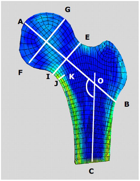
Cross sectional view of a proximal femur FE model indicating definitions of typical proximal femur geometry measures. A–B femoral neck axis length; AOC neck-shaft angle; E–I femoral neck diameter; G–F femoral head diameter; J–K calcar femoral cortex width.

2.7 Reconstruction of known femurs

Individual finite element models of each femur in the training set were reconstructed from the SSDM using (Cootes, Hill, Taylor and Haslam 1994):

$${\mathit{p}}_i=\overline{\mathit{p}}+\mathit{Qb}$$ (5)

where p̄ is the mean shape and bone density model, Q contains the shape model eigenvectors q_i

$$\mathit{Q}=({\mathit{q}}_1\mid {\mathit{q}}_2\dots \mid {\mathit{q}}_{n-1})$$ (6)

for n-1 of non-zero shape model eigenvalues and

$$\mathit{b}={\mathit{Q}}^T({\mathit{p}}_i-\overline{\mathit{p}})$$ (7)

2.8 Reconstruction of an unknown femur

The ability of the statistical shape model to reconstruct an unknown or previously unseen proximal femur was quantified using a leave one out analysis (Cootes, Hill, Taylor and Haslam 1994). In this analysis, the shape model was reformulated using all but one femur in the training set and the resulting eigenmodes were then used to reconstruct the remaining “unknown” femur using a modified version of Eq. 5:

$${\mathit{p}}_u={\overline{\mathit{p}}}^{\prime }+{\mathit{Q}}^{\prime }{\mathit{b}}^{\prime }$$ (8)

where p_u is the unknown femur shape and density vector, p̄′ is the mean shape and density vector of the training set leaving one femur out, and b′ are shape parameters.. The SSDM parameter values, b′, , that minimize the square root of the sum of the squares of the differences between the original shape and density vector of the unknown femur and the SSMD model predicted shape and density vector of the unknown femur (Eq. 8) were determined using non-linear optimization (Mathcad, v.13, PTC, Needham, MA). Error between the original finite element shape and density vector and the SSDM predicted shape and density vector was defined as the difference between corresponding shape and density vector elements of the original vector and the SSDM predicted vector.

3. Results

Principal component analysis of the statistical shape and density model demonstrated that 78% of the variation in the set of 7 human proximal femur finite element models was captured by the first three independent modes of variation (eigenmodes) (Figure 6).

Figure 6.

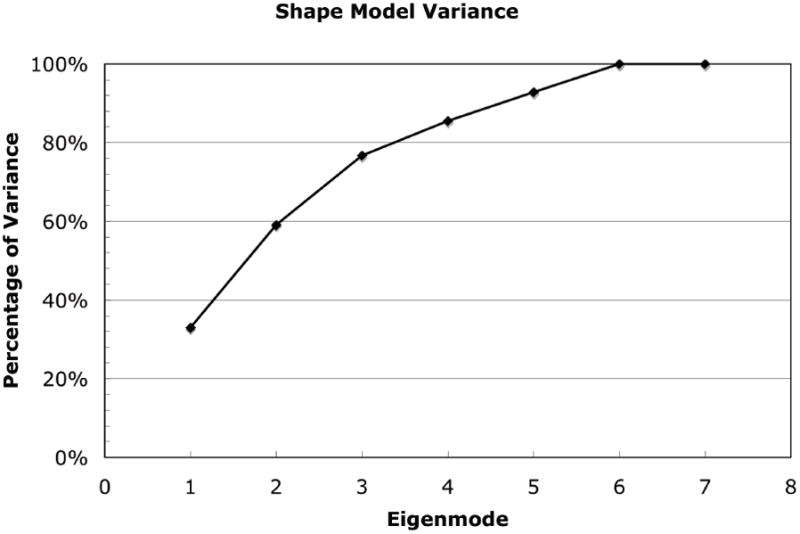
Percentage of total cadaver femur training set variance explained by statistical shape and density model (SSDM) eigenmodes. Nearly 80% of the total variance in proximal femur shape and bone density distribution can be explained by three independent shape and density model eigenmodes. 100% of the variance in the training set is explained by 6 eigenodes.

A +1 SD variation from the mean shape and density distribution due to the first eigenmode resulted in an increase in proximal femur neck axis length, a decrease in neck-shaft angle, increases in both the femoral neck and femoral head diameter, and a decrease in calcar femoral cortex width whereas a −1 SD perturbation resulted in the opposite effect (Figure 7). Shape and density variations due to the second eigenmode had the opposite effect of the first eigenmode. Shape changes of the proximal femur due to the third eignmode for the neck axis length and neck-shaft angle generally followed those changes due to the second mode of variation and in most measures, the changes were of slightly lower magnitude (Figure 8).

Figure 7.

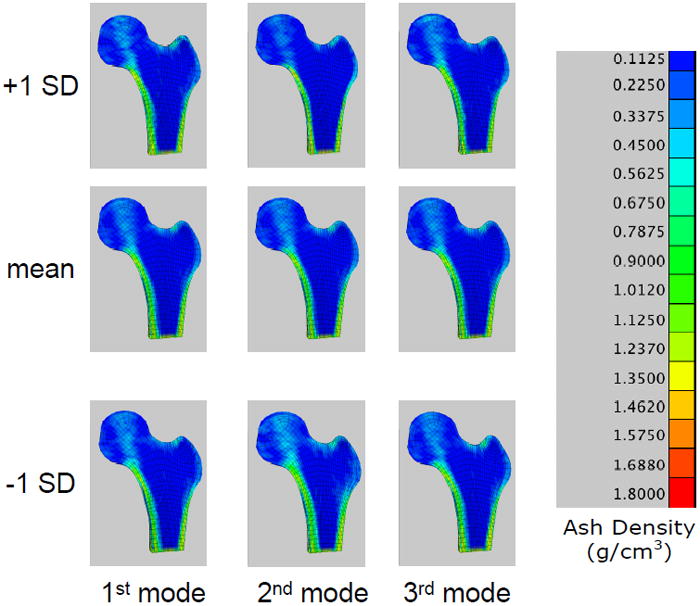
Finite element models constructed from the statistical shape and density model of the femur training set. Fringe levels indicate apparent bone ash density. Center: FE model representing the mean shape and bone density distribution; Top: FE model representing the mean plus 1 SD of the first three eigenmodes; Bottom: mean minus 1 SD of the first three eigenmodes.

Figure 8.

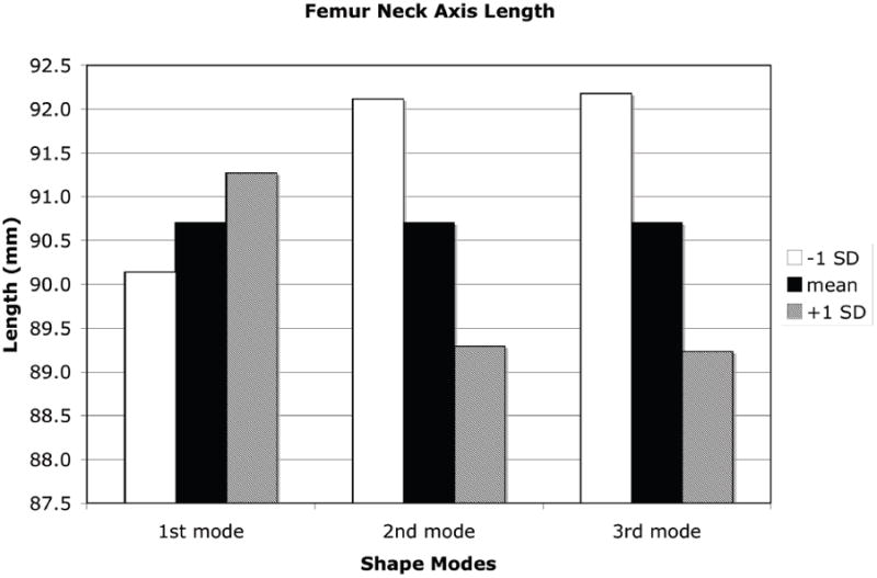
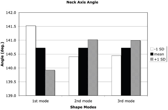
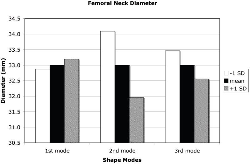
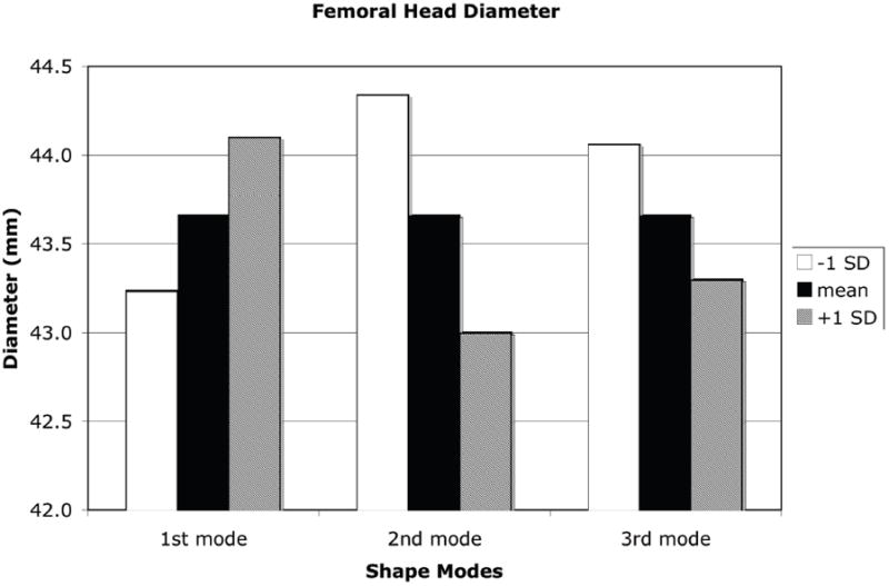
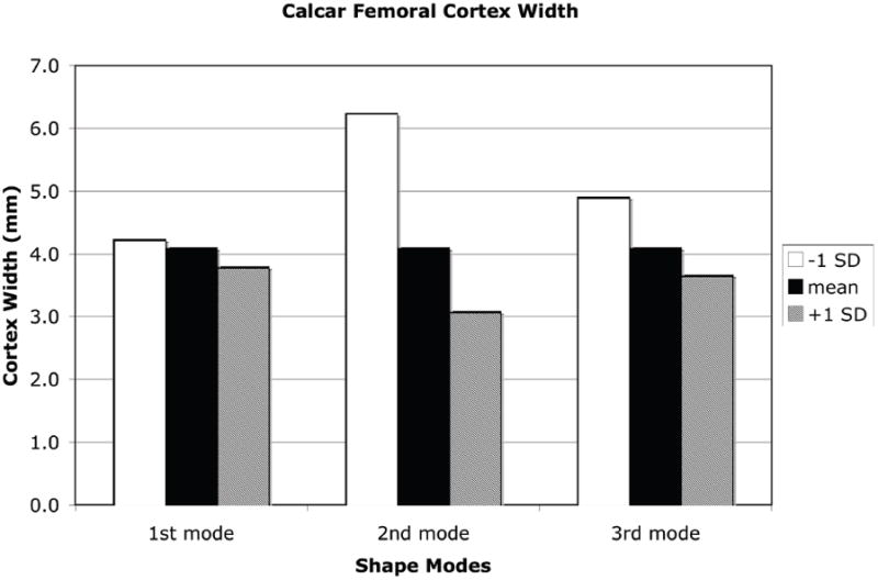
Measures of proximal femur geometry determined for finite element models based on the statistical shape model of the proximal femur. The principal modes of variation from the mean represented by the shape model eigenvalues and eigenvectors generally have no direct physical meaning. However, by tracking the locations of specific points in the FE models that represent common measures of proximal femur geometry, the physical significance of each eigenmode can be discerned. (a): Proximal femur neck axis length; (b): Proximal femur neck axis angle; (c): Proximal femur neck axis diameter; (d): Femoral head diameter; (e): Calcar femoral cortex width.

Variations from the mean shape and density distribution described by the major eigenmodes of the SSDM resulted in significant changes in the simulated fall loading response of the proximal femur (Figure 9). The mean shape and density model resulted in a predicted maximum force of 1590 N. The shape and density variations due to the first eigenmode resulted in an increase in predicted peak force to 1996 N for a mean −1 SD variation and a peak force of 1727 N for a mean + 1 SD variation. Shape and bone density changes due to the second eigenmode has the greatest effect on the model predicated peak force ranging from 4693 N for the mean −1 SD perturbation to 524 N for the mean + 1 SD perturbation.

Figure 9.

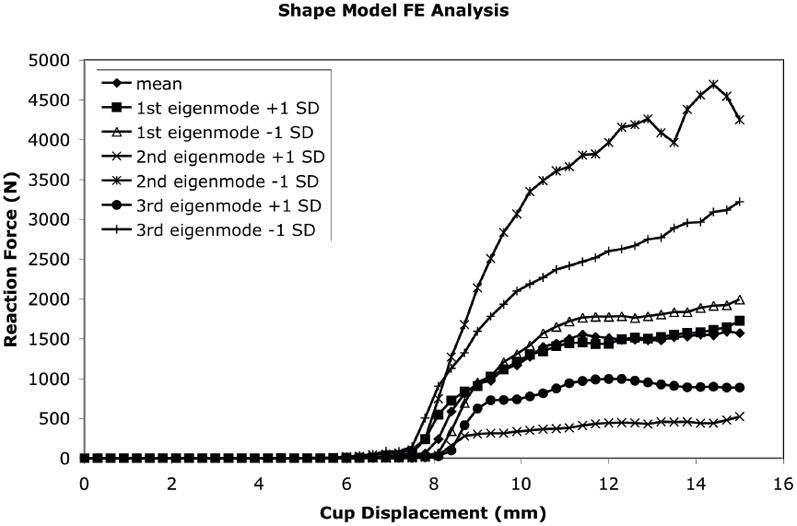
The effect of each independent SSDM eigenmode on the predicted force displacement behavior of the proximal femur in a simulated fall loading condition.

The SSDM was used to reconstruct an individual femur contained within the training set with high accuracy. Using all principal components, the maximum spatial error between the SSDM derived FE model and the original finite element model of the femur was 0.009 mm with an average error of 9.0E-5 mm and the maximum bone density error was 0.0031 g/cm³ with an average error of 9.4E-6 g/cm³. Using a decreasing number of eigenmodes to reconstruct the femur finite element model, the spatial error increased to a maximum of less than 0.5 mm with an average error of 5.9E-3 mm and the bone density error increased to a maximum of 2 g/cm³ with an average of 0.013 g/cm³ when only one eigenmode was used (Figure 10). The shape and bone density distribution of a previously unseen femur was approximated using the SSDM reformulated using all but one femur FE model (defined as the “unknown” femur). The maximum spatial error between the original FE model of the unknown femur and the shape model approximated femur was 2.813 mm with an average error of 0.016 mm (Figure 11a). The maximum bone density error was 0.796 g/cm³ with an average error of 0.037 g/cm³ (Figure 11b).

Figure 10.

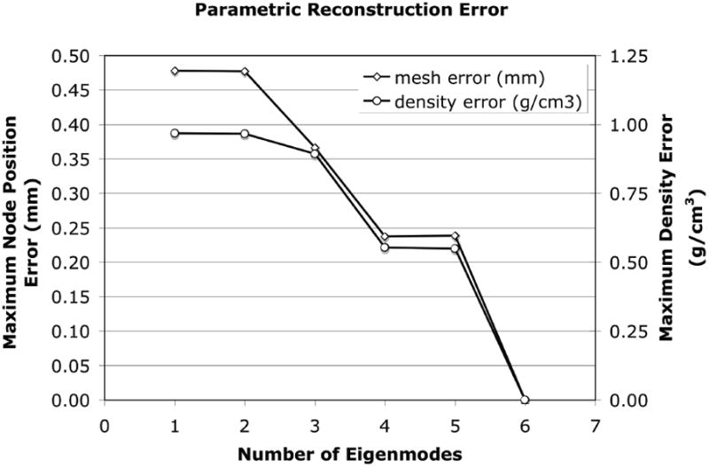
Maximum error between the SSDM derived parametric three dimensional finite element model and the individual femur FE model constructed directly from the QCT image data.

Figure 11.

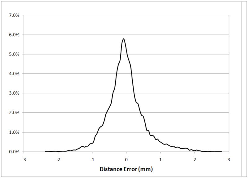
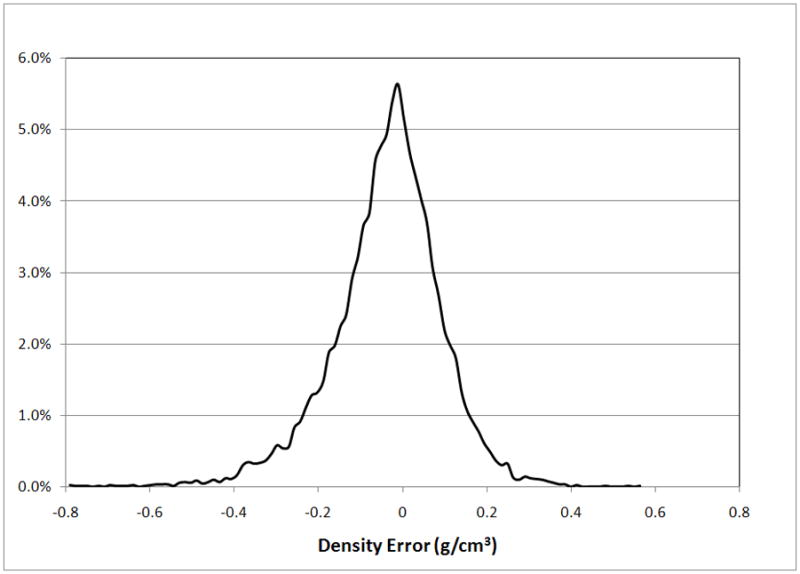
The statistical shape and density model was used to describe an “unknown” femur and the performance was quantified using measures of error. (a) Distribution of spatial mesh error. (b) Distribution of mesh density error.

4. Discussion

A parametric finite element modeling procedure based on statistical shape modeling was developed to model complex shape and bone density variations of a group of cadaver proximal femurs. The statistical shape and density model (SSDM) compactly and efficiently describes the mean and variability in the proximal femur geometry and bone density distribution for the given set of cadaveric femurs using a reduced variable space. The SSDM was used to efficiently re-construct high-fidelity finite element models of individual femurs within the training set with a high degree of accuracy. The parametric finite element modeling procedure was also used to construct a finite element model of an “unknown” femur by varying the SSDM independent parameters to minimize the difference between the SSDM model approximated femur and the actual femur model. The traditional statistical shape modelling approach allows investigations related to geometry variation in a range of musculoskeletal applications including investigating osteoarthritis risk (Bredbenner et al. 2010)) and guiding implant design (Fitzpatrick et al. 2008). In the present study, the SSDM is constructed using a finite element model of each individual femur in the training set, differing from the traditional application of statistical shape modeling in which image data alone is used to construct the shape model. By using a 3D finite element model derived from clinical image data for each femur in the training set, the resulting SSDM can be used to directly construct high fidelity engineering models of the proximal femur; these models can then be used to evaluate the effect of specific variations in bone shape and bone density on predicted bone strength. Since the variability in shape and density distribution of the proximal femur is represented by a set of uncorrelated, independent variables defined by the eigenmodes of the statistical shape and density model, specific combinations of eigenmodes can be used to reconstruct finite element models of an individual femurs and the resulting model used to assess bone strength.

A limitation of the current SSDM is the small number of femurs in the training set. If the femurs in the SSDM training set do not adequately represent shape and density variations in the population of interest, the resulting SSDM will not adequately reconstruct unknown femurs that significantly differ from those within the training set with a high level of accuracy. To overcome this limitation, a larger number of femurs should be included in the training set. The existing SSDM can be updated by reformulating the model to include additional femurs along with the existing set.

The finite element model representing the mean − 1 SD variation in the second eigenmode resulted in an increase in neck angle length, decrease in neck-shaft angle, increase in neck diameter, and an increase in cortex width (Figure 6), all of which have been shown to decrease fracture risk (Center et al. 1998, Crabtree et al. 2002, El-Kaissi et al. 2005, Gnudi et al. 1999, Patron et al. 2006, Pulkkinen, Eckstein, Lochmuller, Kuhn and Jamsa 2006, Pulkkinen, Partanen, Jalovaara and Jamsa 2004, Specker and Binkley 2005). This independent mode of variation (eigenmode) resulted in the greatest predicted maximum load in a simulated fall configuration (Figure 7). Thus, this modeling approach directly relates variations in bone geometry and bone density to bone strength through a high fidelity predictive engineering model. The advantage of the approach described herein is that a physics based predictive finite element model is used to directly assess bone strength, rather than a statistical correlation based on epidemiological data of fracture incidents, bone density measures, and geometry in a given population.

In an investigation employing similar FE-based statistical shape modelling methods to investigate fracture risk, a SSDM was created using QCT data for 21 human cadaver femurs (although the pointwise elastic modulus distribution was used in the formulation, rather than the pointwise BMD distribution used in the present study) (Bryan et al. 2009). The multivariate parameter space of the resulting shape and modulus model was sampled using a Monte Carlo approach and a set of 1000 “virtual femurs” were created within the variability bounds of the shape and modulus model. This interesting study predicted that 28 of the 1000 FE models were at highest risk of fracture due to fall loading and that the overall percentage of cortical bone in the femur played a large role in differentiating between failed and non-failed femurs. However, it would seem that, as in the present study, variability in the multivariate parameter space is limited due to the creation of the SSDM from a small set of femurs (n=21), meaning that the 1000 virtual FE models simulate a group of individuals with relatively similar femur geometry and BMD distribution. Furthermore, it is unclear how the choice of an elastic material model, rather than a more realistic nonlinear material model, would affect the FE results during simulation of overload fracture.

In summary, a statistical shape and density modeling approach was implemented to define a parametric representation of proximal femur geometry and bone density distribution. The SSDM was used to describe the major modes of variation of proximal femur geometry and bone density distribution within the training set of cadaver femurs using a small number of independent modes. The SSDM derived finite element models demonstrated the effect of the major modes of variation in shape and bone density on predicted bone strength. By determining the optimal combination of eigenmodes, a finite element model of a previously unseen femur was constructed. The application of this method to reconstruct the three dimensional shape and bone density distribution of the proximal femur from ubiquitous clinical data such as DXA scans has the potential to significantly improve the assessment of an individual’s risk of bone fracture.

References

- Bauer DC, Ewing SK, Cauley JA, Ensrud KE, Cummings SR, Orwoll ES. Quantitative ultrasound predicts hip and non-spine fracture in men: the MrOS study. Osteoporos Int. 2007;18(6):771–777. doi: 10.1007/s00198-006-0317-5. [DOI] [PubMed] [Google Scholar]
- Benameur S, Mignotte M, Labelle H, De Guise JA. A hierarchical statistical modeling approach for the unsupervised 3-D biplanar reconstruction of the scoliotic spine. IEEE Trans Biomed Eng. 2005;52(12):2041–2057. doi: 10.1109/TBME.2005.857665. [DOI] [PubMed] [Google Scholar]
- Bessho M, Ohnishi I, Matsuyama J, Matsumoto T, Imai K, Nakamura K. Prediction of strength and strain of the proximal femur by a CT-based finite element method. J Biomech. 2007;40(8):1745–1753. doi: 10.1016/j.jbiomech.2006.08.003. [DOI] [PubMed] [Google Scholar]
- Bessho M, Ohnishi I, Okazaki H, Sato W, Kominami H, Matsunaga S, Nakamura K. Prediction of the strength and fracture location of the femoral neck by CT-based finite-element method: a preliminary study on patients with hip fracture. J Orthop Sci. 2004;9(6):545–550. doi: 10.1007/s00776-004-0824-1. [DOI] [PubMed] [Google Scholar]
- Brechbuhler C, Gerig G, Kubler O. Parameterization of closed surfaces for 3-D shape-description. Computer Vision and Image Understanding. 1995;61:154–170. [Google Scholar]
- Bredbenner TL, Bartels KA, Havill LM, Nicolella DP. Summer Bioengineering Conference. Amelia Island, FL: American Society of Mechanical Engineers; Probabilistic shape-based finite element modeling of baboon femurs. [Google Scholar]
- Bredbenner TL, Eliason TD, Potter RS, Mason RL, Havill LM, Nicolella DP. Statistical shape modeling describes variation in tibia and femur surface geometry between Control and Incidence groups from the osteoarthritis initiative database. J Biomech. 2010;43(9):1780–1786. doi: 10.1016/j.jbiomech.2010.02.015. [DOI] [PMC free article] [PubMed] [Google Scholar]
- Bryan R, Nair PB, Taylor M. Use of a statistical model of the whole femur in a large scale, multi-model study of femoral neck fracture risk. J Biomech. 2009;42(13):2171–2176. doi: 10.1016/j.jbiomech.2009.05.038. [DOI] [PubMed] [Google Scholar]
- Burge R, Dawson-Hughes B, Solomon DH, Wong JB, King A, Tosteson A. Incidence and economic burden of osteoporosis-related fractures in the United States, 2005–2025. J Bone Miner Res. 2007;22(3):465–475. doi: 10.1359/jbmr.061113. [DOI] [PubMed] [Google Scholar]
- Center JR, Nguyen TV, Pocock NA, Noakes KA, Kelly PJ, Eisman JA, Sambrook PN. Femoral neck axis length, height loss and risk of hip fracture in males and females. Osteoporos Int. 1998;8(1):75–81. doi: 10.1007/s001980050051. [DOI] [PubMed] [Google Scholar]
- Cody DD, Gross GJ, Hou FJ, Spencer HJ, Goldstein SA, Fyhrie DP. Femoral strength is better predicted by finite element models than QCT and DXA. J Biomech. 1999;32(10):1013–1020. doi: 10.1016/s0021-9290(99)00099-8. [DOI] [PubMed] [Google Scholar]
- Cootes TF, Hill A, Taylor CJ, Haslam J. Use of active shape models for locating structure in medical images. Image and Vision Computing. 1994;12:355–365. [Google Scholar]
- Crabtree NJ, Kroger H, Martin A, Pols HA, Lorenc R, Nijs J, Stepan JJ, Falch JA, Miazgowski T, Grazio S, Raptou P, Adams J, Collings A, Khaw KT, Rushton N, Lunt M, Dixon AK, Reeve J. Improving risk assessment: hip geometry, bone mineral distribution and bone strength in hip fracture cases and controls. The EPOS study. European Prospective Osteoporosis Study. Osteoporos Int. 2002;13(1):48–54. doi: 10.1007/s198-002-8337-y. [DOI] [PubMed] [Google Scholar]
- Davies RH, Twining CJ, Cootes TF, Waterton JC, Taylor CJ. A minimum description length approach to statistical shape modeling. IEEE Trans Med Imaging. 2002;21(5):525–537. doi: 10.1109/TMI.2002.1009388. [DOI] [PubMed] [Google Scholar]
- Dornaika F, Ahlberg J. Fitting 3D face models for tracking and active appearance model training. Image and Vision Computing. 2006;24(9):1010–1024. [Google Scholar]
- El-Kaissi S, Pasco JA, Henry MJ, Panahi S, Nicholson JG, Nicholson GC, Kotowicz MA. Femoral neck geometry and hip fracture risk: the Geelong osteoporosis study. Osteoporos Int. 2005;16(10):1299–1303. doi: 10.1007/s00198-005-1988-z. [DOI] [PubMed] [Google Scholar]
- Ferrarini L, Palm WM, Olofsen H, van Buchem MA, Reiber JH, Admiraal-Behloul F. Shape differences of the brain ventricles in Alzheimer’s disease. Neuroimage. 2006;32(3):1060–1069. doi: 10.1016/j.neuroimage.2006.05.048. [DOI] [PubMed] [Google Scholar]
- Fitzpatrick CK, FitzPatrick DP, Auger DD. Size and shape of the resection surface geometry of the osteoarthritic knee in relation to total knee replacement design. Proc Inst Mech Eng H. 2008;222(6):923–932. doi: 10.1243/09544119JEIM332. [DOI] [PubMed] [Google Scholar]
- Frost ML, Blake GM, Fogelman I. A comparison of fracture discrimination using calcaneal quantitative ultrasound and dual X-ray absorptiometry in women with a history of fracture at sites other than the spine and hip. Calcif Tissue Int. 2002;71(3):207–211. doi: 10.1007/s00223-001-2074-y. [DOI] [PubMed] [Google Scholar]
- Genant HK, Lang TF, Engelke K, Fuerst T, Gluer C, Majumdar S, Jergas M. Advances in the noninvasive assessment of bone density, quality, and structure. Calcif Tissue Int. 1996;59(Suppl 1):S10–15. doi: 10.1007/s002239900169. [DOI] [PubMed] [Google Scholar]
- Gnudi S, Gualtieri G, Malavolta N. Simultaneous densitometry and quantitative bone sonography in the estimation of osteoporotic fracture risk. Br J Radiol. 1998;71(846):625–629. doi: 10.1259/bjr.71.846.9849385. [DOI] [PubMed] [Google Scholar]
- Gnudi S, Ripamonti C, Gualtieri G, Malavolta N. Geometry of proximal femur in the prediction of hip fracture in osteoporotic women. Br J Radiol. 1999;72(860):729–733. doi: 10.1259/bjr.72.860.10624337. [DOI] [PubMed] [Google Scholar]
- Gonnelli S, Cepollaro C, Gennari L, Montagnani A, Caffarelli C, Merlotti D, Rossi S, Cadirni A, Nuti R. Quantitative ultrasound and dual-energy X-ray absorptiometry in the prediction of fragility fracture in men. Osteoporos Int. 2005;16(8):963–968. doi: 10.1007/s00198-004-1771-6. [DOI] [PubMed] [Google Scholar]
- Jiang C, Giger ML, Kwak SM, Chinander MR, Martell JM, Favus MJ. Normalized BMD as a predictor of bone strength. Acad Radiol. 2000;7(1):33–39. doi: 10.1016/s1076-6332(00)80441-9. [DOI] [PubMed] [Google Scholar]
- Johnell O, Kanis JA, Oden A, Sernbo I, Redlund-Johnell I, Petterson C, De Laet C, Jonsson B. Mortality after osteoporotic fractures. Osteoporos Int. 2004;15(1):38–42. doi: 10.1007/s00198-003-1490-4. [DOI] [PubMed] [Google Scholar]
- Kanis JA. Assessing the risk of vertebral osteoporosis. Singapore Med J. 2002a;43(2):100–105. [PubMed] [Google Scholar]
- Kanis JA. Diagnosis of osteoporosis and assessment of fracture risk. Lancet. 2002b;359(9321):1929–1936. doi: 10.1016/S0140-6736(02)08761-5. [DOI] [PubMed] [Google Scholar]
- Kanis JA, Johnell O, Oden A, Sembo I, Redlund-Johnell I, Dawson A, De Laet C, Jonsson B. Long-term risk of osteoporotic fracture in Malmo. Osteoporos Int. 2000;11(8):669–674. doi: 10.1007/s001980070064. [DOI] [PubMed] [Google Scholar]
- Kanis JA, Oden A, Johnell O, De Laet C, Jonsson B, Oglesby AK. The components of excess mortality after hip fracture. Bone. 2003;32(5):468–473. doi: 10.1016/s8756-3282(03)00061-9. [DOI] [PubMed] [Google Scholar]
- Kaus MR, Pekar V, Lorenz C, Truyen R, Lobregt S, Weese J. Automated 3-D PDM construction from segmented images using deformable models. IEEE Trans Med Imaging. 2003;22(8):1005–1013. doi: 10.1109/TMI.2003.815864. [DOI] [PubMed] [Google Scholar]
- Keller TS. Predicting the compressive mechanical behavior of bone. J Biomech. 1994;27(9):1159–1168. doi: 10.1016/0021-9290(94)90056-6. [DOI] [PubMed] [Google Scholar]
- Keyak JH. Improved prediction of proximal femoral fracture load using nonlinear finite element models. Med Eng Phys. 2001;23(3):165–173. doi: 10.1016/s1350-4533(01)00045-5. [DOI] [PubMed] [Google Scholar]
- Keyak JH, Meagher JM, Skinner HB, Mote CD., Jr Automated three-dimensional finite element modelling of bone: a new method. J Biomed Eng. 1990;12(5):389–397. doi: 10.1016/0141-5425(90)90022-f. [DOI] [PubMed] [Google Scholar]
- Keyak JH, Rossi SA, Jones KA, Skinner HB. Prediction of femoral fracture load using automated finite element modeling. J Biomech. 1998;31(2):125–133. doi: 10.1016/s0021-9290(97)00123-1. [DOI] [PubMed] [Google Scholar]
- Koikkalainen J, Hirvonen J, Nyman M, Lotjonen J, Hietala J, Ruotsalainen U. Shape variability of the human striatum--Effects of age and gender. Neuroimage. 2007;34(1):85–93. doi: 10.1016/j.neuroimage.2006.08.039. [DOI] [PubMed] [Google Scholar]
- Lecouvet FE, Malghem J, Michaux L, Michaux JL, Lehmann F, Maldague BE, Jamart J, Ferrant A, Vande Berg BC. Vertebral compression fractures in multiple myeloma. Part II. Assessment of fracture risk with MR imaging of spinal bone marrow. Radiology. 1997;204(1):201–205. doi: 10.1148/radiology.204.1.9205247. [DOI] [PubMed] [Google Scholar]
- Les CM, Keyak JH, Stover SM, Taylor KT, Kaneps AJ. Estimation of material properties in the equine metacarpus with use of quantitative computed tomography. J Orthop Res. 1994;12(6):822–833. doi: 10.1002/jor.1100120610. [DOI] [PubMed] [Google Scholar]
- Lorenz C, Krahnstöver N. Generation of point-based 3D statistical shape models for anatomical objects. Computer Vision and Image Understanding. 2000;77(2):175–191. [Google Scholar]
- Lotz JC, Cheal EJ, Hayes WC. Fracture prediction for the proximal femur using finite element models: Part I--Linear analysis. J Biomech Eng. 1991;113(4):353–360. doi: 10.1115/1.2895412. [DOI] [PubMed] [Google Scholar]
- Lotz JC, Cheal EJ, Hayes WC. Stress distributions within the proximal femur during gait and falls: implications for osteoporotic fracture. Osteoporos Int. 1995;5(4):252–261. doi: 10.1007/BF01774015. [DOI] [PubMed] [Google Scholar]
- Majumdar S, Lin J, Link T, Millard J, Augat P, Ouyang X, Newitt D, Gould R, Kothari M, Genant H. Fractal analysis of radiographs: assessment of trabecular bone structure and prediction of elastic modulus and strength. Med Phys. 1999;26(7):1330–1340. doi: 10.1118/1.598628. [DOI] [PubMed] [Google Scholar]
- Mauch S. A fast algorithm for computing the closest point and distance function [Google Scholar]
- Melton LJ., 3rd Adverse outcomes of osteoporotic fractures in the general population. J Bone Miner Res. 2003;18(6):1139–1141. doi: 10.1359/jbmr.2003.18.6.1139. [DOI] [PubMed] [Google Scholar]
- Nicholson PH, Lowet G, Cheng XG, Boonen S, van der Perre G, Dequeker J. Assessment of the strength of the proximal femur in vitro: relationship with ultrasonic measurements of the calcaneus. Bone. 1997;20(3):219–224. doi: 10.1016/s8756-3282(96)00370-5. [DOI] [PubMed] [Google Scholar]
- Oden ZM, Selvitelli DM, Bouxsein ML. Effect of local density changes on the failure load of the proximal femur. J Orthop Res. 1999;17(5):661–667. doi: 10.1002/jor.1100170507. [DOI] [PubMed] [Google Scholar]
- Patron MS, Duthie RA, Sutherland AG. Proximal femoral geometry and hip fractures. Acta Orthop Belg. 2006;72(1):51–54. [PubMed] [Google Scholar]
- Pulkkinen P, Eckstein F, Lochmuller EM, Kuhn V, Jamsa T. Association of geometric factors and failure load level with the distribution of cervical vs. trochanteric hip fractures. J Bone Miner Res. 2006;21(6):895–901. doi: 10.1359/jbmr.060305. [DOI] [PubMed] [Google Scholar]
- Pulkkinen P, Partanen J, Jalovaara P, Jamsa T. Combination of bone mineral density and upper femur geometry improves the prediction of hip fracture. Osteoporos Int. 2004;15(4):274–280. doi: 10.1007/s00198-003-1556-3. [DOI] [PubMed] [Google Scholar]
- Rajamani K, Nolte L, Styner M. A novel approach to anatomical structure morphing for intraoperative visualization; Medical Imaging Computing and Computer-Assisted Intervention -- MICCAI 2004, Pt 2, Proceedings; Berlin: Springer; 2004. [Google Scholar]
- Rao A, Babalola K, Rueckert D. Biomedical Image Registration. Berlin/Heidelberg: Springer; 2006. Canonical correlation analysis of subcortical brain structures using non-rigid registration; pp. 66–74. [Google Scholar]
- Rehman Q, Lang T, Modin G, Lane NE. Quantitative computed tomography of the lumbar spine, not dual x-ray absorptiometry, is an independent predictor of prevalent vertebral fractures in postmenopausal women with osteopenia receiving long-term glucocorticoid and hormone-replacement therapy. Arthritis Rheum. 2002;46(5):1292–1297. doi: 10.1002/art.10277. [DOI] [PubMed] [Google Scholar]
- Ross PD. Clinical consequences of vertebral fractures. Am J Med. 1997;103(2A):30S–42S. doi: 10.1016/s0002-9343(97)90025-5. discussion 42S–43S. [DOI] [PubMed] [Google Scholar]
- Rueckert D, Frangi AF, Schnabel JA. Automatic construction of 3-D statistical deformation models of the brain using nonrigid registration. IEEE Trans Med Imaging. 2003;22(8):1014–1025. doi: 10.1109/TMI.2003.815865. [DOI] [PubMed] [Google Scholar]
- Shan ZY, Parra C, Ji Q, Jain J, Reddick WE. A knowledge-guided active model method of cortical structure segmentation on pediatric MR images. J Magn Reson Imaging. 2006;24(4):779–789. doi: 10.1002/jmri.20688. [DOI] [PubMed] [Google Scholar]
- Specker B, Binkley T. High parity is associated with increased bone size and strength. Osteoporos Int. 2005;16(12):1969–1974. doi: 10.1007/s00198-005-1978-1. [DOI] [PubMed] [Google Scholar]
- Stewart A, Kumar V, Reid DM. Long-term fracture prediction by DXA and QUS: a 10-year prospective study. J Bone Miner Res. 2006;21(3):413–418. doi: 10.1359/JBMR.051205. [DOI] [PubMed] [Google Scholar]
- Sweeney AT, Malabanan AO, Blake MA, Weinberg J, Turner A, Ray P, Holick MF. Bone mineral density assessment: comparison of dual-energy X-ray absorptiometry measurements at the calcaneus, spine, and hip. J Clin Densitom. 2002;5(1):57–62. doi: 10.1385/jcd:5:1:057. [DOI] [PubMed] [Google Scholar]
- Tabensky AD, Williams J, DeLuca V, Briganti E, Seeman E. Bone mass, areal, and volumetric bone density are equally accurate, sensitive, and specific surrogates of the breaking strength of the vertebral body: an in vitro study. J Bone Miner Res. 1996;11(12):1981–1988. doi: 10.1002/jbmr.5650111221. [DOI] [PubMed] [Google Scholar]
- Taddei F, Cristofolini L, Martelli S, Gill HS, Viceconti M. Subject-specific finite element models of long bones: An in vitro evaluation of the overall accuracy. J Biomech. 2006;39(13):2457–2467. doi: 10.1016/j.jbiomech.2005.07.018. [DOI] [PubMed] [Google Scholar]
- Taddei F, Pancanti A, Viceconti M. An improved method for the automatic mapping of computed tomography numbers onto finite element models. Med Eng Phys. 2004;26(1):61–69. doi: 10.1016/s1350-4533(03)00138-3. [DOI] [PubMed] [Google Scholar]
- Taneichi H, Kaneda K, Takeda N, Abumi K, Satoh S. Risk factors and probability of vertebral body collapse in metastases of the thoracic and lumbar spine. Spine (Phila Pa 1976) 1997;22(3):239–245. doi: 10.1097/00007632-199702010-00002. [DOI] [PubMed] [Google Scholar]
- Testi D, Viceconti M, Cappello A, Gnudi S. Prediction of hip fracture can be significantly improved by a single biomedical indicator. Ann Biomed Eng. 2002;30(6):801–807. doi: 10.1114/1.1495866. [DOI] [PubMed] [Google Scholar]