Comparison of multi‐subject ICA methods for analysis of fMRI data

Abstract

Spatial independent component analysis (ICA) applied to functional magnetic resonance imaging (fMRI) data identifies functionally connected networks by estimating spatially independent patterns from their linearly mixed fMRI signals. Several multi‐subject ICA approaches estimating subject‐specific time courses (TCs) and spatial maps (SMs) have been developed, however, there has not yet been a full comparison of the implications of their use. Here, we provide extensive comparisons of four multi‐subject ICA approaches in combination with data reduction methods for simulated and fMRI task data. For multi‐subject ICA, the data first undergo reduction at the subject and group levels using principal component analysis (PCA). Comparisons of subject‐specific, spatial concatenation, and group data mean subject‐level reduction strategies using PCA and probabilistic PCA (PPCA) show that computationally intensive PPCA is equivalent to PCA, and that subject‐specific and group data mean subject‐level PCA are preferred because of well‐estimated TCs and SMs. Second, aggregate independent components are estimated using either noise‐free ICA or probabilistic ICA (PICA). Third, subject‐specific SMs and TCs are estimated using back‐reconstruction. We compare several direct group ICA (GICA) back‐reconstruction approaches (GICA1‐GICA3) and an indirect back‐reconstruction approach, spatio‐temporal regression (STR, or dual regression). Results show the earlier group ICA (GICA1) approximates STR, however STR has contradictory assumptions and may show mixed‐component artifacts in estimated SMs. Our evidence‐based recommendation is to use GICA3, introduced here, with subject‐specific PCA and noise‐free ICA, providing the most robust and accurate estimated SMs and TCs in addition to offering an intuitive interpretation. Hum Brain Mapp, 2011. © 2010 Wiley Periodicals, Inc.

INTRODUCTION

In functional magnetic resonance imaging (fMRI) of the brain, spatial independent component analysis (ICA) is commonly used to separate spatially independent patterns from their linearly mixed blood‐oxygen‐level‐dependent (BOLD) signals via maximization of mutual independence among components. Unlike voxel‐wise univariate methods such as regression analysis or Kolmogorov‐Smirnov statistics, ICA does not naturally generalize to a method suitable for drawing inferences about groups of subjects. For example, when using the general linear model, the investigator specifies the regressors of interest, and so drawing inferences about group data comes naturally, since all individuals in the group share the same regressors. In ICA, by contrast, different individuals in the group will have time course and spatial map differences, and they will be sorted differently, so it is not immediately clear how to draw inferences about group data using ICA. To address these issues, several multi‐subject ICA approaches have been proposed [Beckmann et al.,2005; Calhoun et al.,2001a,b,2004a; Esposito et al.,2005; Guo and Pagnoni,2008; Lukic et al.,2002; Schmithorst and Holland,2004; Svensén et al.,2002]. The various approaches differ in terms of how the data are organized prior to the ICA, how group and subject estimates are computed, what types of output are available (for example, single subject contributions, group averages, etc.), and how the statistical inference is made.

As we discuss in a recent review article, group ICA approaches can be organized into five categories [Calhoun et al.,2009]. Some approaches use single‐subject ICA and then attempt to combine the output into a group post hoc by using approaches such as self‐organized clustering or spatial correlation of the components [Calhoun et al.,2001a; Esposito et al.,2005]. This has the advantage of allowing for unique spatial and temporal features, but has the disadvantage that since the data are noisy the components are not necessarily unmixed in the same way for each subject. The other four approaches involve an ICA computed on the group data as a whole. Temporal concatenation [Calhoun et al.,2001b] and spatial concatenation [Svensén et al.,2002] have both been examined. The advantage of these approaches is that they perform one ICA, which can then be divided into subject‐specific parts, hence the comparison of subject differences within a component is straightforward. The temporal concatenation approach discussed in this article allows for unique time courses (TCs) for each subject, but assumes common aggregate spatial maps (SMs) whereas the spatial concatenation approach not discussed here allows for unique SMs but assumes common TCs. Although they are really just two different approaches for organizing the data, temporal concatenation appears to work better for fMRI data [Schmithorst and Holland,2004] most likely because the temporal variations (and hence nonstationarity) in the ICA time courses are much larger than the variation in the spatial maps at conventional field strengths of 3T and below [see for example, Calhoun et al.,2008a].

Temporal concatenation has been widely used for group ICA of fMRI data and has been implemented initially in the group ICA of fMRI toolbox (GIFT) [Calhoun,2004] for Matlab (http://icatb.sourceforge.net/) and more recently in the multivariate exploratory linear optimized decomposition into independent components (MELODIC) software (http://www.fmrib.ox.ac.uk/fsl/). The GIFT software additionally implements a back‐reconstruction step which produces subject‐specific images, which has been noted to show accurate estimation of variations in subject‐specific TCs and SMs through a simulation example [Calhoun et al.,2001b]. This enables a comparison of both the TCs and the SMs for one group or multiple groups [Calhoun et al.,2008b]. The approach implemented in GIFT thus trades‐off the use of a common model for the SMs against the difficulties of combining single subject ICA. An intermediate approach would use temporal concatenation separately for each group [Celone et al.,2006], although in this case, matching the components post hoc becomes again necessary. Yet another approach involves averaging the data prior to performing ICA [Schmithorst and Holland,2004]. This approach is less computationally demanding, but makes a more stringent assumption of having a common TC and a common SM. In [Guo and Pagnoni,2008], an extended group tensor model was presented to estimate group‐specific temporal responses and common spatial maps. CanICA [Varoquaux et al.,2010] uses canonical correlation analysis with multi‐subject fMRI data to estimate only the aggregate SM from the ICA step. Hence CanICA does not provide a way to estimate subject‐specific TCs and SMs. Finally, tensor decompositions (also known as multidimensional, multi‐way, or N‐way decompositions), have received renewed interest recently, although their adaptation to group and multi‐group fMRI data is still being explored. One approach is based upon a three‐dimensional tensor that has been developed to estimate a single spatial, temporal, and subject‐specific “mode” for each component to attempt to capture the multidimensional structure of the data in the estimation stage [Beckmann and Smith,2005]. This approach, however, may not work as well (without additional preprocessing) if the TCs between subjects are different, such as in a resting state study in which the time course is obviously not synchronized between subjects as it is in a task paradigm with similar timing between subjects.

In this article, we compare three subject‐level principal component analysis (PCA) dimension reduction strategies with four multi‐subject ICA methods using both simulated data and real fMRI data collected during a task. Figure 1 illustrates the group ICA process and the areas of focus of this article, and Table I summarizes notation. There are commonly two PCA reduction steps, one at the subject level and a second at the group level. The three subject‐level PCA strategies we compare are subject‐specific [Calhoun,2004; Calhoun et al.,2001b], spatial concatenation [Beckmann et al.,2005], and group data mean in MELODIC v3.0 [Beckmann and Smith,2004]. We also compare PCA with probabilistic PCA (PPCA). We also compare noise‐free ICA with probabilistic ICA (PICA) [Beckmann and Smith,2003; Calhoun,2004]. To construct subject‐level TCs and associated SMs, the multi‐subject ICA methods we compare are three variations on PCA‐based direct back‐reconstruction approach group ICA (GICA) [Calhoun et al.,2001b,2002] and a least squares‐based indirect back‐reconstruction approach spatio‐temporal regression (STR, or dual regression) [Beckmann et al.,2009; Calhoun et al.,2004b]. We present comparisons of PCA, ICA, and back‐reconstruction strategies and give evidence‐based recommendations. Some mathematical details illustrating key results are left to the Appendix.

Figure 1.

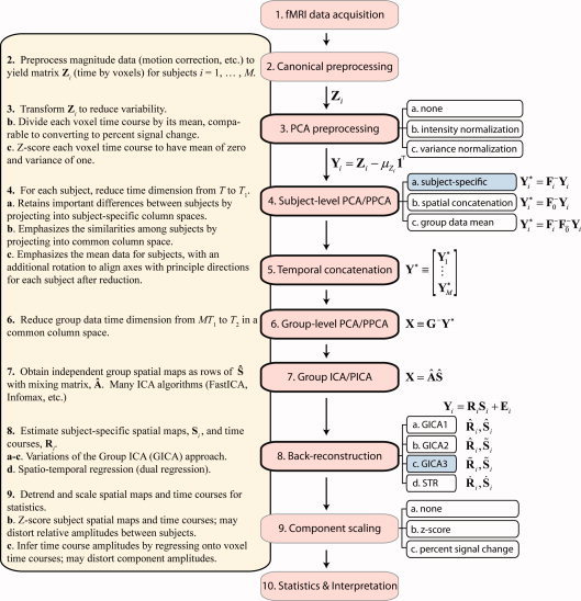
Common steps and choices in a multi‐subject ICA analysis. In this article, we discuss Steps (3)–(8), with attention to (4) subject‐level PCA and (8) back‐reconstruction. The findings in this article recommend using PCA with subject‐specific subject‐level PCA reduction and noise‐free ICA with GICA3 back‐reconstruction. [Color figure can be viewed in the online issue, which is available at wileyonlinelibrary.com.]

Table I.

Summary of subject‐level PCA and back‐reconstruction method notation discussed here, see Figure 1 for context

Figure 1, Step 4
Data Reduction	Strategy
PCA	Singular value decomposition (SVD) of covariance matrix
PPCA	Factor analysis where noise covariance is σ2 I
Figure 1, Step 4
Subject‐level PCA	Reduced data	PCA Calculation
Subject‐specific	Y ${}_{\mathit{\text{i}}}^{\text{*}}$ = F ${}_{\mathit{\text{i}}}^{\text{−}}$ Y i	F ${}_{\mathit{\text{i}}}^{\text{−}}$ = F ${}_{\mathit{\text{i}}}^{\text{T}}$ from cov of Y i
Spatial‐concatenation	Y ${}_{\mathit{\text{i}}}^{\text{*}}$ = F ${}_{\text{0}}^{\text{−}}$ Y i	F ${}_{\text{0}}^{\text{−}}$ = F ${}_{\text{0}}^{\text{T}}$ from cov of [Y 1, ··· ,Y M]
Group data mean	Y ${}_{\mathit{\text{i}}}^{\text{*}}$ = F ${}_{\mathit{\text{i}}}^{\text{−}}$ F ${}_{\text{0}}^{\text{−}}$ Y i	= F ${}_{\text{0}}^{\text{T}}$ from cov of , and rotation F ${}_{\mathit{\text{i}}}^{\text{−}}$ from cov of Y i
Figure 1, Step 7
Source Separation	Strategy
ICA	Maximization of mutual independence among components
PICA	Independent factor analysis with isotropic noise
Figure 1, Step 8	Let subject data be the product of TC and SM:		Y i = R i S i + E i
Back‐reconstruction	Time course (TC)	Spatial map (SM)	Column space
GICA1	R̂ i ≡ F i G i Â	Ŝ i = Â − G ${}_{\mathit{\text{i}}}^{\text{−}}$ F ${}_{\mathit{\text{i}}}^{\text{T}}$ Y i	Ŷ i = R̂ i Ŝ i = P${}_{\mathit{\text{C}}\text{(}\mathbf{\text{F}}{}_{\mathit{\text{i}}}\mathbf{\text{G}}{}_{\mathit{\text{i}}}\text{)}}$ Y i
First method, based on partitioning group PCA matrix G
GICA2	R̂ i from GICA1	S̃ i from GICA3	Not a projection
Mixture of GICA1 and GICA3
GICA3	R̃ i ≡ F i (G ${}_{\mathit{\text{i}}}^{\text{T}}$)− Â	S̃ i = Â − G ${}_{\mathit{\text{i}}}^{\text{T}}$ F ${}_{\mathit{\text{i}}}^{\text{T}}$ Y i	Ỹ i ≡ R̃ i S̃ i = P${}_{\mathit{\text{C}}\text{(}\mathbf{\text{F}}{}_{\mathit{\text{i}}}\mathbf{\text{G}}{}_{\mathit{\text{i}}}\text{)}}$ Y i
Introduced here, modification of GICA1 partitioning inverse of group PCA matrix G −, sum of estimated subject SMs is aggregate SM (13), PCA‐reduced data matches PCA‐reduced product of estimated TCs and SMs (33)
STR	Ṙ i = Y i Ŝ −	Ṡ i = Ṙ ${}_{\mathit{\text{i}}}^{\text{−}}$ Y i	Ẏ i = Ṙ i Ṡ i = P${}_{\mathit{\text{C}}\text{(}\mathbf{\text{Y}}{}_{\mathit{\text{i}}}\mathbf{\text{Ŝ}}{}^{\text{−}}\text{)}}$ Y i, complicated (35)
Uses least squares multiple regression to estimate subject‐specific TCs from aggregate SM, then estimates subject‐specific SMs from TCs

MATERIALS AND METHODS

PCA

Principal component analysis is necessary for the multi‐subject ICA methods described here so we begin with a short description [Pearson,1901]. For observed vectors (a time series for each voxel), Z _v, v = 1,…,V, subtract the mean and concatenate column wise into Y = [Z ₁,…,Z _V] − Z 1 ^T, where 1 ^T is the transpose of a column vector of 1s. Let the T‐dimensional, zero mean, random row vector Y have singular value decomposition (SVD) of its covariance matrix, Σ_Y = F _T D _T F ${}_{\text{T}}^{\mathit{\text{T}}}$. Order the eigenvectors in the order of descending eigenvalues to form an ordered orthogonal basis with the first eigenvector specifying the direction of largest variance of the data. Let F and D be the matrices of the first T ₁ ordered eigenvectors and eigenvalues, that is

(1)

The data can be represented by the first T ₁ basis vectors of the orthogonal basis as Y ^* = F ^T Y, the PCA‐reduced data. The best linear predictor (BLP) of Y is “Y‐smile”, and is optimal in mean squared error (MSE), where P _C(F) = FF ^T is the perpendicular projection operator (PPO) onto the column space of F, C(F), since F is orthonormal. The Moore‐Penrose pseudoinverse simplifies to F ⁻ = (F ^T F)⁻¹ F ^T = F ^T.

Data

Let Y _i be the T‐by‐V magnitude data matrix for subject i containing the preprocessed and spatially normalized data with rows of zero mean, where T time points over V voxels are collected on M subjects (Figure 1, Steps 1, 2, and 3). Let Y ≡ [Y ${}_{\text{T}}^{\text{1}}$,…,Y ${}_{\text{T}}^{\mathit{\text{M}}}$]^T be the temporally concatenated subject data. The data are compressed via two PCA dimension reduction steps. The subject‐level PCA has computational benefits due to dimension reduction and the denoising benefits of projecting the data onto the principal subspace of the data. Group‐level PCA is required for the multi‐subject ICA methods presented here to reduce the dimension of the data to the number of components estimated with ICA.

Subject‐Level PCA

To make the estimation computationally tractable it is common to first perform a subject‐level PCA dimension reduction (Figure 1, Step 4).

Subject‐specific PCA

Let Y ${}_{\text{*}}^{\mathit{\text{i}}}$ = F ${}_{\text{−}}^{\mathit{\text{i}}}$ Y _i be the T ₁‐by‐V PCA‐reduced data for subject i, where F ${}_{\text{−}}^{\mathit{\text{i}}}$ = F ${}_{\text{T}}^{\mathit{\text{i}}}$ is the T ₁‐by‐T standardized reducing matrix and T ₁ is the number of principal components retained for each subject. Let

(2)

be the MT ₁‐by‐V time‐concatenated aggregate data (Figure 1, Step 5). The predicted data after dimension reduction are .

There are a number of methods for determining the effective dimension of the data, among them are the information theoretic approaches such as an information criterion (AIC), Kullback information criterion (KIC), and the minimum description length (MDL) [also called the Bayesian information criterion (BIC)] [Li et al.,2007]. In (2) T ₁ could be determined for each F ${}_{\text{−}}^{\mathit{\text{i}}}$ separately, but later in the back‐reconstruction of the subject‐specific TCs and SMs each individual will have the same number of components dependent on the number of components in the ICA. Therefore, it is preferred to use a common T ₁ for all F ${}_{\text{−}}^{\mathit{\text{i}}}$, i = 1,…,M, as in [Calhoun et al.,2001b,2002]. Subject‐specific data reduction privileges differences among subjects.

Subject spatially concatenated PCA

First, calculate F ${}_{\text{−}}^{\text{0}}$ = F ${}_{\text{T}}^{\text{0}}$, the T ₁‐by‐T standardized reducing matrix of the T‐by‐MV spatially concatenated aggregate data [Y ₁,…,Y _M]. Second, temporally concatenate the data in Y ^* as in (2) using the common reducing matrix so F ${}_{\text{−}}^{\mathit{\text{i}}}$ ≡ F ${}_{\text{−}}^{\text{0}}$, i = 1,…,M [Beckmann et al.,2005]. The predicted data after dimension reduction is . This strategy forces each subjects' data in Y ^* to share a common column space. Spatial‐concatenation privileges commonalities among subjects.

Group data mean PCA

First, calculate the subject mean dataset, , and perform PCA of Y to obtain = , the T ₁‐by‐T standardized reducing matrix. Then, a second subject‐level standard PCA is performed to rotate each of the matrices to be aligned with the principal directions of each subject‐reduced data to have the T ₁‐by‐T reduced data, F ${}_{\text{−}}^{\mathit{\text{i}}}$ F ${}_{\text{−}}^{\text{0}}$ Y _i, as implemented in MELODIC 3.0 (Release 4.0, Aug 2007, downloaded Dec 2009) [Beckmann and Smith,2004]. The predicted data after dimension reduction is . By using the mean data matrix, the PCA is performed on the mean of the random variables instead of on the random variables themselves. This strategy is similar to spatial‐concatenation except rather than using MV observations to estimate the covariance matrix for PCA, it uses V mean vectors over the M subjects. Group data mean privileges commonalities among subjects.

Group‐Level PCA

Let the T ₂‐by‐V PCA‐reduced aggregate data be

(3)

where G ⁻ is the T ₂‐by‐MT ₁ standardized reducing matrix (Figure 1, Step 6). Ideally, T ₂ ≡ C is selected to be the true number of independent components (ICs) for all subjects, and each subject has the same components. The predicted subject‐compressed data is

(4)

The predicted subject data is

(5)

In practice, for real fMRI data, subjects will each have their own number of components. How to best choose the number of components at the group level to best represent the subjects is a choice, and we use an implementation of MDL [Li et al.,2007].

ICA

Following square noise‐free spatial ICA estimation [Hyvärinen et al.,2001], we can write

(6)

where the generative linear latent variables  and Ŝ are the T ₂‐by‐T ₂ mixing matrix related to subject TCs and the T ₂‐by‐V aggregate SM, respectively (Figure 1, Step 7). In this form of spatial ICA, there is no aggregate or group‐level TC. Below we use multi‐subject ICA methods to estimate subject‐specific TCs, R _i, and SMs, S _i, i = 1,…,M, conditional on the ICA estimates and PCA reductions of the data. Although a tensor approach to multi‐subject ICA provides an aggregate TC [Beckmann and Smith,2005], it is only sensible when the TCs are common for all subjects, such as in a task.

Subject Back‐Reconstruction Methods

We present four heuristic methods for estimating subject‐specific TCs and SMs for fMRI data (Figure 1, Step 8). The three GICA methods are based on PCA compression and projection [Calhoun,2004; Calhoun et al.,2001b,2002]. Note that the GICA methods are numbered chronologically but presented in an order for clear exposition. The STR least squares method uses PCA compression indirectly through the estimate of the aggregate SM [Beckmann et al.,2009; Calhoun et al.,2004b].

GICA3

Consider a heuristic method such that natural estimates lead to certain desirable properties. For each subject, i = 1,…,M, let the subject data Y _i be the product of the subject‐specific TC and SM, R _i and S _i, plus error, E _i,

(7)

In GICA3, assume that subject‐specific TCs are the subject‐specific PCA back‐projected mixing matrix,

(8)

Then for subject i, PCA compression of the data gives Y ${}_{\text{*}}^{\mathit{\text{i}}}$ = F ${}_{\text{T}}^{\mathit{\text{i}}}$ Y _i, leading to the compressed data for each subject relating to the common mixing matrix with a subject‐specific SM,

(9)

where A = G ${}_{\text{T}}^{\mathit{\text{i}}}$ F ${}_{\text{T}}^{\mathit{\text{i}}}$ R _i is the common mixing matrix and S _i is the subject‐specific SM. Aggregating over subjects gives the group reduced data related to the aggregate SM,

(10)

where the aggregate SM is the sum of the subject‐specific SMs, . In noise‐free ICA we estimate the mixing matrix and aggregate SM in (10),

(11)

From (11) the natural estimate of the subject‐specific SM substitutes our estimate of A into either defining relationship (7) or by solving X _i = G ${}_{\text{T}}^{\mathit{\text{i}}}$ F ${}_{\text{T}}^{\mathit{\text{i}}}$ Y _i = Â S _i for S _i,

(12)

Note that we have exactly that the aggregate SM is the sum of the subject‐specific SMs,

(13)

Further, from (8) the natural estimator of subject‐specific TC R _i substitutes the estimate of A to give

(14)

Note that the key assumption and definition in this derivation are (8) and (12) leading to the following desirable properties. The product of each subject‐specific TC and SM is a perpendicular projection of the data onto the PCA column space, Ỹ _i ≡ R̃ _i S̃ _i = P ${}_{\mathit{\text{C}}\text{(}\mathbf{\text{F}}{}_{\mathit{\text{i}}}\mathbf{\text{G}}{}_{\mathit{\text{i}}}\text{)}}$ Y _i [see (30)]. The PCA compressed fitted values are exactly the PCA compressed data X, that is, the fitted values and data agree in the PCA space [see (31)]. The fitted compressed values, X̃ _i ≡ Â S̃ _i = X _i, are a product of the subject‐specific TC and SM [see (32)], and similarly for the mean fitted compressed value, [see (33)]. Thus, it is the amount of information retained in the PCA steps that largely determines the subject‐specific TC and SM estimates.

GICA1

The group ICA (GICA) method provided the first method based on ICA for estimating subject‐specific TCs and SMs [Calhoun et al.,2001b,2002]. The differences in GICA1 from GICA3 come from a different partitioning of group‐level PCA reducing matrix G. Following GICA3, replace the assumption regarding subject‐specific TCs in (8) with

(15)

and the definition of subject‐specific SMs in (12) with

(16)

As such, the aggregate SM does not equal the sum of the subject‐specific SMs. Still, from (15) the natural estimator of subject‐specific TC R _i is

(17)

Note that the assumption and definition in this derivation, (15) and (16), leads to the following properties. The product of each subject‐specific TC and SM is a perpendicular projection of the data onto the PCA column space Ỹ _i = R̃ _i S̃ _i = P ${}_{\mathit{\text{C}}\text{(}\mathbf{\text{F}}{}_{\mathit{\text{i}}}\mathbf{\text{G}}{}_{\mathit{\text{i}}}\text{)}}$ Y _i. The PCA compressed fitted values are exactly the PCA compressed data X, that is, the fitted values and data agree in the PCA space, similar to (31). However, the difference from GICA3 is that the fitted compressed values, X̂ _i, are not a product of the subject‐specific TC and SM, , thus also . Note that the fitted values as the product of the subject‐specific TCs and SMs for GICA1 and GICA3 are equivalent, R̂ _i Ŝ _i = R̃ _i S̃ _i, both being perpendicular projections of the data onto C(F _i G _i).

GICA2

Because GIFT software implemented GICA2 from versions v1.01b to v2.0c, we present this hybrid method [Calhoun,2004]. Following GICA3, use the assumption regarding subject‐specific TCs as in GICA1 in (15) giving the natural estimator for R _i as R̂ _i ≡ F _i G _i Â, but the definition of subject‐specific SMs as in GICA3 in (12) giving the estimator for S _i as S̃ _i = Â ⁻ G ${}_{\text{T}}^{\mathit{\text{i}}}$ F ${}_{\text{T}}^{\mathit{\text{i}}}$ Y _i. The subject‐specific fitted values are no longer a projection, because G ${}_{\text{T}}^{\mathit{\text{i}}}$ G _i ≠ I, since G _i is not orthonormal. Given these fitted values, recompressing them with PCA does not give the same X as compressing the original data. But, as in GICA3, the sum of the subject‐specific maps is the aggregate spatial map . As in GICA3, the fitted compressed values are a product of the subject‐specific TCs and SMs and therefore the mean fitted compressed value also matches the mean compressed data.

STR (dual regression)

Spatio‐temporal regression (STR), or dual regression, is an indirect back‐reconstruction approach using least squares to estimate the subject‐specific TCs and SMs [Beckmann et al.,2009; Calhoun et al.,2004b]. Given ICA results, as in (11) or PICA [Beckmann and Smith,2004], STR first estimates subject‐specific TCs, Ṙ _i, then SMs, Ṡ _i, via multiple regression. We note that because ICA limits the amount of correlation between the aggregate SM components (i.e., if two component TCs were highly correlated they would have been grouped into the same component), the concern of colinearity between the variables appears mitigated, but as we later show, variation among subjects may have subject‐specific SMs that are a mixture of a few aggregate SMs because of TCs that are more highly correlated for some subjects. To motivate this method we begin again by letting Y _i = R _i S _i + E _i. The first assumption is that all subjects share a common SM, S _i ≡ S, i = 1,…,M. Then, from the ICA in (6), substitute Ŝ for S and take the transpose of the equation for

(18)

Least squares estimation for TC R ${}_{\text{T}}^{\mathit{\text{i}}}$ gives Ṙ ${}_{\text{T}}^{\mathit{\text{i}}}$ = (Ŝ Ŝ ^T)⁻¹ Ŝ Y ${}_{\text{T}}^{\mathit{\text{i}}}$, or the transpose [Calhoun et al.,2004b],

(19)

As an aside, note that the transpose of the product of the aggregate SM and subject‐specific TC is a perpendicular projection of the data onto C(Ŝ ^T), Ŝ ^T Ṙ ${}_{\text{T}}^{\mathit{\text{i}}}$ = Ŝ ^T(Ŝ Ŝ ^T)⁻¹ Ŝ Y ${}_{\text{T}}^{\mathit{\text{i}}}$ = P ${}_{\mathit{\text{C}}\text{(}\mathbf{\text{Ŝ}}{}^{\text{T}}\text{)}}$ Y ${}_{\text{T}}^{\mathit{\text{i}}}$. To estimate each subject‐specific SM, S _i, the original assumption of common SMs is relaxed. Conditional on the estimated subject‐specific TC, Ṙ _i, let

(20)

with E[E _2i] = 0. Least squares estimation for S _i gives

(21)

The product of each subject‐specific TC and SM gives

(22)

where P ${}_{\mathit{\text{C}}\text{(}\mathbf{\text{Ṙ}}{}_{\mathit{\text{i}}}\text{)}}$ = P ${}_{\mathit{\text{C}}\text{(}\mathbf{\text{Y}}{}_{\mathit{\text{i}}}\mathbf{\text{Ŝ}}{}^{\text{−}}\text{)}}$ is a PPO onto C(Y _i Ŝ ⁻) [see (34)]. This column space is much different from in GICA1 or GICA3 where they depend only on the PCA reduction matrices. This method indirectly uses compression through the V‐by‐T ₂ dimensional Ŝ ⁻, which was estimated through ICA using the PCA compressed data. In contrast to (13) for GICA3, the sum of the subject‐specific SMs relate to the aggregate SM in a way that is not clear how to interpret,

(23)

These estimates of Ṙ _i and Ṡ _i require contradictory assumptions regarding the SMs, where the SMs are assumed to be the common aggregate map to estimate subject‐specific TCs, then distinct subject‐specific SMs are estimated.

By personal communication (Stephen Smith), both regressions are meant to include a column of ones in the design matrix, leading to an estimate different from GICA1, where (18) and (19) are replaced by

(24)

and where (20) and (21) are replaced by

(25)

It is unclear what the ramifications are of including additional regressors, such as motion parameters, in the design matrices and thus such practice requires careful examination before recommendation.

Probabilistic PCA and ICA

An alternative to the noise‐free methods presented above are so‐called probabilistic methods (Figure 1, Steps 4, 6, and 7).

PPCA

Probabilistic PCA (PPCA) is related to factor analysis [Bartholomew and Knott,1987; Basilevsky,1994] where the noise covariance of PPCA is the more restrictive σ² I rather than in factor analysis as diag (σ${}_{\text{2}}^{\text{1}}$,…,σ${}_{\text{2}}^{\mathit{\text{T}}}$) [Tipping and Bishop,1999]. The maximum likelihood estimate for σ² is the average loss of variance (eigenvalues) over the lost dimensions. As σ² → 0, the PPCA represents the orthogonal projection into the standard PCA space. With σ² > 0, it is an oblique projection skewed toward the origin.

PICA

Probabilistic ICA (PICA), also known as noisy ICA or independent factor analysis, attempts to generalize ICA to include noise [Attias,1999]. Although there are many algorithms for PICA they all implicitly assume the identifiability of the mixing matrix A and/or the noise covariance C _noise [Attias,1999; De Lathauwer et al.,1996; Hyvärinen,1999a,b; Moulines et al.,1997]. Although A is identifiable, C _noise is not uniquely identifiable, though the elements are bounded, thus the primary criticism of PICA is the ambiguity in assigning variance between the independent components and the noise process, introducing an ambiguity into the results [Davies,2004]. The strategy implemented in FSL/MELODIC software [Beckmann and Smith,2004] to overcome the nonidentifiability issue is to assume that the noise covariance is isotropic, C _noise = σ${}_{\text{2}}^{\text{noise}}$ I, allowing convergence of parameter estimates [Davies,2004]. Even with the isotropic assumption, the decomposition into independent components is unique only if no more source signals are extracted from the data than exist, thus the algorithm may fail to converge if too many components are specified.

These probabilistic versions of PCA and ICA have been applied to fMRI data [Beckmann and Smith,2004], and are implemented in the FSL/MELODIC software. Therefore, we have incorporated their PPCA and PICA code into GIFT to investigate their properties compared to their noise‐free counterparts.

Experiments

Simulated data

A simulated fMRI‐like dataset in Figure 2 representing sources of interest and artifacts is used as the true common set of sources among subjects. Let R and S denote the true group “mean” TC and SM matrices. Among the C = 8 source SMs, one is task‐related (1), two are transiently task‐related (2 and 6), and five are artifact‐related (3, 4, 5, 7, and 8), where five are super‐Gaussian (1, 2, 5, 6, and 8), two are sub‐Gaussian (3 and 7), and one is Gaussian (4). Thirty‐two, M = 32, realizations of subject data are simulated from the group “mean” by adding subject‐specific Gaussian noise to the TCs and SMs and by varying the amplitude of the task‐related TCs. Specifically, let r _c be column c of R and let s′_c be row c of s, then subject‐specific data with no noise (nn) are generated with

(26)

where φ_ic ∼ Normal (0,σ${}_{\text{2}}^{\mathbf{\text{r}}\mathit{\text{ic}}}$) for c = 1,2,3,6 and equal to 0 otherwise, θ′_ic ∼ Normal (0,σ${}_{\text{2}}^{\mathbf{\text{s}}\mathit{\text{ic}}}$) for c = 1,2,3,5,6,7,8 and equal to 0 otherwise, g _ic = Uniform(0.25,1.75) for c = 1,2,6 and equal to 1 otherwise, with σ${}_{\text{2}}^{\mathbf{\text{r}}\mathit{\text{ic}}}$ and σ${}_{\text{2}}^{\mathbf{\text{s}}\mathit{\text{ic}}}$ equal to the signal variation for component c divided by (2, 4, 8, and 16) for subjects 1–8, 9–16, 17–24, and 25–32, respectively, to provide between‐subject differences. The remaining TCs and SMs are already random between subjects. Also, three subjects have different SMs for the task‐related component: subject 10 has no task‐related TC or SM so has only seven components, subject 20 has an additional disk of activation on the task‐related SM, and subject 30 has only one of the two disks of activation on the task‐related SM.

Figure 2.

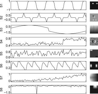
Simulated data time courses and spatial maps. Among the C = 8 source SMs, one is task‐related (1), two are transiently task‐related (2 and 6), and five are artifact‐related (3, 4, 5, 7, and 8), where five are super‐Gaussian (1, 2, 5, 6, and 8), two are sub‐Gaussian (3 and 7), and one is Gaussian (4).

We add Rician noise to the simulated data to represent a realistic SNR [Okada et al.,2005]. In our laboratory for fMRI experiments at 3T with TR = 2 s and TE = 29 ms, and a voxel size of 3.75 mm³ we typically observe a mean SNR = 90. The magnitude of our zero‐mean data is estimated by and the additive factor to scale the data to 2% activation is calculated, . In the image background, with signal equal to zero, the noise mean has a Raleigh distribution and is given by and the SNR for an fMRI image can be defined by SNR = A/μ${}_{\text{background}}^{\text{noise}}$. This implies that . For each element in Y ${}_{\text{nn}}^{\mathit{\text{i}}}$ over time and voxels, Y ${}_{\text{nn}}^{\mathit{\text{i}}}$(t,v), we add noise to obtain , where ν₁ and ν₂ are both distributed as Normal(0,σ${}_{\text{2}}^{\text{noise}}$), giving us simulated “true” data Y _i, i = 1,…,M. Note that with high SNR, Rician data is approximately Gaussian, and therefore this simulation is consistent with the PICA model.

Auditory oddball task data

Twenty‐eight healthy controls were scanned during an auditory oddball task (AOD) consisting of detecting an infrequent sound within a series of regular and different sounds, previously published [Calhoun et al.,2008a]. The participants were instructed to respond as quickly and as accurately as possible with their right index finger every time they heard the target stimulus and not to respond to the nontarget stimuli or the novel stimuli. The stimulus paradigm data acquisition techniques and previously found stimulus‐related activation are described more fully elsewhere [Kiehl et al.,2001,2005]. This data includes 249 time points over 63,533 voxels.

PCA comparisons

We compare the subject‐level PCA dimension reduction techniques by the similarity of the original data matrix Y _i with the PCA reduced then back‐projected estimated data matrix from near (2) using root mean squared error (RMSE) calculated element‐wise as

(27)

where smaller RMSE indicates more similarity. To compare the amount of information lost in subject‐level PCA methods, in (27) Y _i is the original data for subject i and , where F ${}_{\text{−}}^{\mathit{\text{i}}}$ is either subject‐specific reducing matrix, the spatially concatenated PCA reducing matrix, F ${}_{\text{−}}^{\mathit{\text{i}}}$ ≡ F ${}_{\text{−}}^{\text{0}}$, i = 1,…,M, or the group data mean reducing matrix . To compare the information lost overall with the subject‐level and group‐level PCA, we compare the original data Y with the group‐reduced predicted data from (5).

Group ICA comparisons

We compare estimates for the population mean and subject‐specific TCs and SMs. We calculate the mean RMSE over subjects between the estimated and true TCs and SMs, RMSE(R̃ _ic,R _ic) and RMSE(S̃ _ic,S _ic). Time course detrending often removes the mean, the slope, and period π and 2π sines and cosines over the full time course, though we only remove the mean from TCs and SMs in our analyses of the simulated data and the AOD data, and we do not scale by z‐scoring. This preserves the characteristics of the TC estimates.

For the AOD data, we do not know the true TCs and SMs. Therefore, GICA3 and STR will be compared by the difference in TC and SM for the subject most similarly estimated (highest correlation) with the two methods and the subject least similarly estimated (correlation closest to zero).

Simulated resting‐state data

We also simulated a resting‐state paradigm analogous to the task‐related paradigm. Using the same SMs in Figure 2, TCs were simulated for Components 1, 2, and 6 having 0.3–0.4 Hz frequency range (assuming 2‐s TR) and random noise for the remaining components, where cycles differed for each subject with respect to frequency, cycle onset, and inter‐cycle length, with random noise added. The goal is to create time courses for components that are asynchronous among subjects.

Simulated demographic data

For the three task‐related Components (1, 2, and 6), we specify spatial map intensity effects over a mask that depend on a binary (B) covariate (such as gender), a continuous (C) covariate (such as age), and their interaction (B×C). For each of M = 100 subjects we manipulate intensity g _ic in (26),

(28)

where B_ic ∼ Bernoulli(0.5), C_ic ∼ Normal(0,σ${}_{\text{2}}^{\text{C}}$), and e _ic ∼ Normal(0,σ${}_{\text{2}}^{\mathit{\text{ec}}}$). The beta vector for Component 1 is β₁ = [1,−0.4,0.4,0], indicating binary and continuous covariates but no interaction, applied to rectangular spatial mask consisting of the lower spot. The beta vector for Component 2 is β₂ = [1,0,−0.5,0.4] applied to rectangular spatial mask consisting of the pair of oppositely signed spots. The beta vector for Component 6 is β₆ = [1,0.4,0,−0.4] applied to rectangular spatial mask consisting of the upper spot. The remaining components and unmasked regions effectively have a beta of [1,0,0,0]. We set σ${}_{\text{2}}^{\text{C}}$ = 0.5 to allow g _ic to be spread without becoming negative, and σ${}_{\text{2}}^{\mathit{\text{ec}}}$ was 0.05, 0.02, and 0.01 for Components 1, 2, and 6, respectively, for more noise in the more distinct Components 1 and 2, and less noise for Component 6. Finally, “true” t statistics are computed from the true simulated SMs, then t statistics are computed using GICA3 and STR and compared to the “true” t statistics. GICA3 and STR are used after subject‐specific subject‐level PCA with 60 components, eight group‐level PCA components, and noise‐free ICA with 10 runs of ICASSO.

RESULTS

Analysis of Simulated Data

Subject‐level PCA and PPCA methods

For our simulated data, the number of components selected by MDL for each subject was five or six. The information retained is compared for the three subject‐level PCA methods with different numbers of components at each level. Let PCA1 and PCA2 refer to the number of components retained for each subject in the subject‐level PCA and the concatenated data in the group‐level PCA, respectively. A range of components retained for PCA1 (60, 15, 8, 6, and 4) were paired with a range for PCA2 (30, 15, 8, 6, and 4) such that the number retained maintains PCA1 ≥ PCA2. As an aside, for the temporally concatenated group data after the subject‐level PCA with 60 components, MDL estimates four components after the subject‐specific and group data mean subject‐level PCA, whereas MDL estimates seven components after spatial‐concatenation subject‐level PCA. This indicates a consistency between subject‐specific and group data mean in terms of aligning the subject‐level information, whereas there is perhaps some misalignment from spatial‐concatenation which requires more dimensions in the aggregate to capture the dimensionality of the group data.

Figure 3a compares the subject‐specific, spatial‐concatenation, and group data mean approaches for subject‐level PCA plotting the mean of the over all 32 subjects. Subject‐specific reduction retains more information than spatial‐concatenation and group data mean, with information retained decreasing as the number of components decreases. At 60 components, subject‐specific PCA has RMSE of 0.147 [with standard deviation (SD) 0.011], spatial‐concatenation has 0.165 (0.012), and group data mean has 0.175 (0.015).

Figure 3.

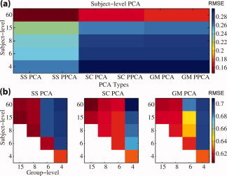
(a) Mean of values for subject‐level PCA/PPCA reduction for a range of components retained using three methods: subject‐specific (SS), spatial‐concatenation (SC), and group data mean (GM). (b) Mean of values for total PCA reduction for a range of components retained at the subject‐level and group‐level. Smaller RMSE indicates more information retained.

Figure 3b compares the overall information reduction from both steps, . For the true number of components (eight) and higher, subject‐specific PCA retains more information than the other methods. But for the estimated number of components (six) and lower, spatial‐concatenation retains more information except for (6,6) where subject‐specific approach has lower RMSE. Four components for the second PCA are too few to retain. For 60 components at the subject level and 6 at the group level RMSE for subject‐specific reduction is 0.689 (SD 0.055), for spatial‐concatenation is 0.617 (0.058), and group data mean is 0.683 (0.055). These results suggest that retaining the same number of components in the subject‐level and group‐level PCAs retain the greatest information, and that the overall information retained is similar between subject‐level reduction methods. However, later we show that for the ICA it is better to retain more components in the subject‐level reduction and close to the true number of components at the group‐level. Also, though these methods retain similar amounts of information after the PCA, the quality of the TCs and SMs differ substantially enough to prefer the subject‐specific or group data mean subject‐level PCA reduction.

The results between PCA and PPCA reduced data matrices differ in RMSE by no more than 10⁻⁷ for any comparison of the simulated or real AOD data, suggesting the results of these two approaches are not different for the application of fMRI data, though there may be cases where they do give different results.

ICA

ICASSO was used to analyze ten runs of the ICA and PICA algorithms to check component stability and that the clusters for both methods were compact [Himberg et al.,2004]. Results of ICASSO suggest that convergence was consistent among runs. We use the Infomax algorithm for ICA because it has been shown to be more consistent than FastICA in repeated runs [Fig. 3, Correa et al.,2007] and does not constrain the demixing matrix to be orthogonal. PICA uses FastICA.

Subject‐specific TC and SM estimation quality

We compare TC and SM quality by calculating the mean RMSE over subjects. We find that the overall lowest RMSE considering both TC and SM estimation is using GICA3 with subject‐specific subject‐level PCA with ICA for most choices of PCA components.

For TCs, Figure 4a shows that GICA3 has lower RMSE than GICA1 and STR when using noise‐free ICA with subject‐specific and group data mean subject‐level PCA for nearly all combinations of PCA components. GICA3 has lower RMSE for noise‐free ICA than for PICA. GICA1 and STR have roughly the same low RMSE over all conditions: all subject‐level PCA methods, ICA and PICA methods, and the number of PCA components retained at subject‐ and group‐levels. STR and GICA1 appear robust to these choices for TCs.

Figure 4.

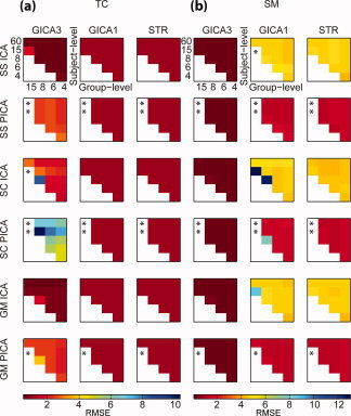
Mean RMSE between estimated and true (a) TC and (b) SM over subjects for the task‐related component (1), RMSE(R̃ _ic,R _ic) and RMSE(S̃ _ic,S _ic), comparing GICA3, GICA1, and STR multi‐subject ICA approaches using subject‐specific (SS), spatial concatenation (SC), and group data mean (GM) subject‐level PCA methods with ICA and PICA. See Table II for more detail. Three cells have been removed because of large values that distorted the scale (TC/SC/ICA/GICA3/15,15; TC/SC/PICA/GICA3/8,8; SM/SS/ICA/GICA1/15,15), other missing values noted with “*” indicate that PICA failed to converge.

For spatial concatenation subject‐level PCA, GICA3 has larger RMSE because the method inflates the amplitude of the TCs for certain subjects, see Figure 5 (but see Table II for similarities if using correlation to evaluate accuracy). For the standard deviation of the TCs, both subject‐specific and group data mean subject‐level PCA methods perform similarly and are close to the truth, whereas spatial concatenation is unpredictably different for each subject. If the TCs are scaled, then the profile of the TCs compared with the truth are similar among all three subject‐level PCA methods. Therefore to estimate the TC amplitude accurately with GICA3, spatial concatenation subject‐level PCA should be avoided.

Figure 5.

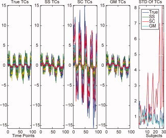
For GICA3 with ICA, the task‐related TC is plotted for the 31 subjects with that component present. The five subplots are the true TCs, the TCs estimated using subject‐level PCA subject‐specific, spatial concatenation, and group data mean, and finally the standard deviation of the TCs for each individual for the first four subplots.

Table II.

Comparisons of the mean RMSE values in Figure 4, and mean correlation, for PCA reduction with 60 subject‐level components and six group‐level components for GICA3 and STR, ICA and PICA, and subject‐specific, spatial concatenation, and group data mean subject‐level PCA

	ICA Method	TC		SM
		GICA3	STR	GICA3	STR
RMSE
Subject‐specific	ICA	0.492 (0.119)	0.986 (0.506)	0.062 (0.015)	4.697 (0.752)
	PICA	2.465 (0.785)	0.923 (0.471)	0.073 (0.009)	1.217 (0.254)
Spatial concatenation	ICA	1.933 (1.842)	0.984 (0.505)	0.118 (0.089)	4.225 (0.629)
	PICA	6.692 (6.492)	0.925 (0.470)	0.080 (0.017)	1.184 (0.203)
Group data mean	ICA	0.528 (0.147)	0.986 (0.506)	0.062 (0.015)	4.629 (0.694)
	PICA	2.420 (0.775)	0.923 (0.471)	0.073 (0.009)	1.190 (0.222)
Correlation
Subject‐specific	ICA	0.843 (0.104)	0.827 (0.159)	0.927 (0.073)	0.903 (0.100)
	PICA	0.800 (0.121)	0.787 (0.176)	0.862 (0.075)	0.825 (0.116)
Spatial concatenation	ICA	0.880 (0.055)	0.806 (0.173)	0.790 (0.184)	0.926 (0.082)
	PICA	0.843 (0.067)	0.753 (0.194)	0.703 (0.202)	0.848 (0.085)
Group data mean	ICA	0.826 (0.099)	0.831 (0.157)	0.925 (0.074)	0.911 (0.093)
	PICA	0.781 (0.117)	0.788 (0.176)	0.860 (0.075)	0.839 (0.106)

Smaller RMSE and larger correlation is better. Values are mean (sd).

For SMs, Figure 4b shows that GICA3 has lower RMSE over all subject‐level PCA methods, ICA and PICA, and all combinations of PCA components. GICA1 and STR have lower RMSE for PICA than ICA. GICA3 appears robust to these choices for SMs.

ICA always converged whereas PICA sometimes failed to converge when the requested number of components was much greater (15) than the true number of components (8), see Figure 4.

To discuss these results at a finer level, recall that PCA1 is the number of components retained at the subject‐level, and PCA2 is for the group‐level. For TCs, GICA3 has lowest RMSE when PCA2 is consistent with MDL (six components), and RMSE increases when PCA1 has very few components, in particular when PCA1 = PCA2 or when PCA1 and PCA2 have too few components. For TCs, STR has lowest RMSE when PCA2 is consistent with MDL (six components), and RMSE increases as PCA2 deviates from the correct number of components. For TCs, GICA1 is similar to STR except, like GICA3, RMSE increases when PCA1 is no more than the number of components that MDL estimates.

Table II provides additional detail for PCA reduction with 60 subject‐level components and six group‐level components for GICA3 and STR for subject‐specific, spatial concatenation, and group data mean subject‐level PCA. Comparisons using mean RMSE reveal that GICA3 has lower RMSE for ICA over PICA for TCs and SMs, except for spatial concatenation SMs. STR has lower RMSE for PICA over ICA for all. GICA3 has lower RMSE than STR for TCs and SMs using ICA, and for SMs using PICA. Overall, GICA3 has lowest RMSE with subject‐specific using ICA. Considering correlation, rather than RMSE, ICA always provides larger correlations than PICA, and GICA3 has larger correlations than STR for subject‐specific and group data mean.

Subject‐specific PCA method effects on TCs and SMs

Though the overall is lower for spatial‐concatenation after group PCA reduction than subject‐specific or group data mean for 60 and six components (see Figure 3b), the quality from the subject‐specific PCA is higher for both the ICA estimation (see Figure 4) and the visual quality of the TC and SM (Figure 6, below).

Figure 6.

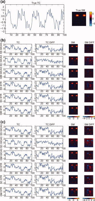
Comparison of TC and SM estimation for the simulated data task‐related component (1) for a subject (12) chosen at random, using subject‐specific (SS), spatial concatenation (SC), and group data mean (GM) subject‐level PCA, (b) noise‐free ICA and (c) PICA, and GICA3 and STR. The true TC and SM for the subject is shown in (a). For the TCs and SMs, the left plot is the estimated value and the right plot is the difference with the true TC (SM) which ideally is flat at zero for both the TC and SM.

Figure 6a shows the true TC and SM for a subject (12) chosen at random, Figure 6b shows the z‐scored scaled estimated TC and SM and the difference between the estimated and true TC and SM using ICA with the three subject‐level PCA methods, and Figure 6c shows the same using PICA. For TCs, differences from the true TCs are smaller for noise‐free ICA than PICA, and GICA3 has smaller differences than STR. For SMs, noise‐free ICA has fewer artifacts than PICA, and GICA3 has fewer artifacts than STR.

ICA and back‐reconstruction method effects on TCs and SMs

Figure 7 compares GICA3 and STR using the simulated data for the task‐related component (1) presenting unthresholded SMs for two subjects selected from the simulated data. Inter‐method spatial correlation between GICA3 with ICA and STR with PICA was used to choose the best‐matching subject (27) and the worst‐matching subject (26). For the most similar subject (27), the SM for GICA3 with ICA and STR with ICA looks very clean for the task‐related component (1), while for STR with PICA there is an artifact of Component 2. Although the TCs look similar between methods, the difference between GICA3 with ICA and STR with PICA reveals the TC for Component 2 associated with the spatial artifact in the SM for STR. For the least similar subject (26) there is stronger task‐related component (1) activation shown in the SM for GICA3 with ICA than for STR with ICA or PICA, and STR with ICA or PICA has an artifact from a different component (4). In the difference SMs, the artifactual component is clear as well as the higher task‐related component activation by GICA3. The GICA3 TC shows stronger task‐related pattern than STR with ICA or PICA and the difference reveals the task‐related component that is stronger for GICA3 and a suggestion of the step‐change artifact from Component 4. Thus, the SMs estimated by GICA3 are in close agreement with the truth and the difference with STR reveals artifacts from the STR method, consistent with previous results in, Table II, Figure 6b, Figure 8, and Figure 9.

Figure 7.

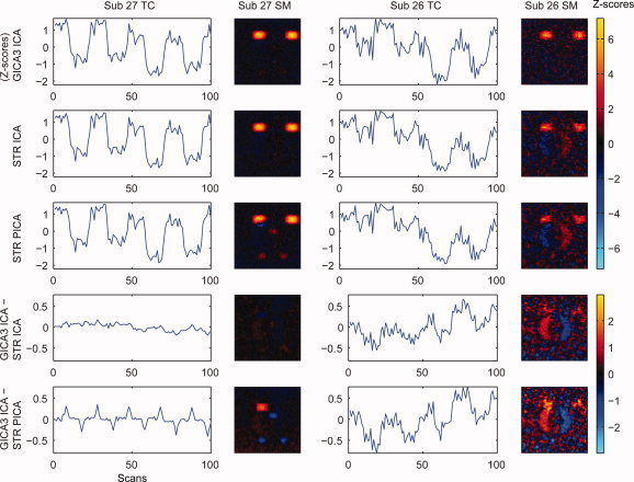
Estimated TCs, SMs, and differences between them for GICA3 with ICA and STR with ICA and PICA for simulated data for the most (27) and least (26) spatially correlated subjects.

Figure 8.

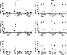
Comparisons of the subject‐specific TC and SM using mean (with NPBS 95% CI) for RMSE(R̃ _ic,R _ic) and RMSE(S̃ _ic,S _ic) for TCs and SMs (notation for GICA3), closer to zero is better. Solid circles are ICA and open circles are PICA, and G3, G1, and SR are GICA3, GICA1, and STR, respectively.

Figure 9.

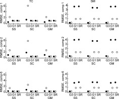
Comparisons of the RMSE between the mean true and mean estimated TC and SM, and (notation for GICA3), closer to zero is better. Solid circles are ICA and open circles are PICA.

Comparisons with good PCA component selection

We make additional comparisons over all combinations of the three task‐related Components (1, 2, and 6), the back‐reconstruction methods (GICA3, GICA1, and STR), and subject‐level PCA methods, while choosing to retain 60 components for the subject‐level PCA and 6 for the group‐level PCA since that provides good estimation for the TCs and SMs (see Figure 4).

For comparisons of the subject‐specific TCs and SMs we calculate the mean RMSE over subjects between the estimated and true subject‐specific TCs and SMs. In Figure 8, the means are displayed with nonparametric bootstrap standard errors (NPBS SEs). For TCs, GICA3 has much lower RMSE with ICA than with PICA. GICA1 and STR are effectively equivalent and the ICA/PICA choice is not important. With ICA, the TC quality does not greatly differ among GICA3, GICA1, and STR for the subject‐specific and group data mean subject‐level PCA strategies, whereas we have previously observed that spatial‐concatenation loses amplitude information with GICA3. For SMs, GICA3 has extremely low RMSE compared with GICA1 and STR, and for GICA1 and STR PICA has much lower RMSE than using ICA. These results are consistent with Figure 4.

For comparisons of the mean TC and SM over subjects we calculate the RMSE between the mean of the estimates and the true mean TC and SM, and , for GICA3 for example. In Figure 9, we observe similar trends as in Figure 8 with GICA1 and STR matching almost exactly for mean TC and SM.

For comparisons of the sum of the subject‐specific SMs equating to the aggregate SM in (13) we calculate the RMSE between the sum of the subject‐specific SMs and the ICA aggregate SM, , for GICA3 for example. Figure 10 indicates that GICA3 matches almost exactly whereas GICA1 and STR, which are not required to fulfill this condition, are far from it.

Figure 10.

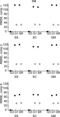
Comparison of desired property of the sum of the subject‐specific SMs equaling the ICA aggregate SM, (notation for GICA3), closer to zero is better. Solid circles are ICA and open circles are PICA.

Iterating STR until convergence

One could consider iterating STR until a convergence criterion is met for the subject‐specific TCs or SMs. That is, we start with (19) to solve for Ṙ _i given Y _i and Ŝ ⁻, then use (21) to solve for Ṡ _i given Y _i and Ṙ ${}_{\text{−}}^{\mathit{\text{i}}}$, then repeat by substituting Ṡ _i for Ŝ in (19), stopping when sequential solutions of either Ṙ _i or Ṡ _i do not differ much. This strategy could distance the results from the contradictory assumptions of common and subject‐specific SM, but the convergence properties of such a solution are currently not well understood and beyond the scope of this article. In Figure 11 we use the same subject (12) from Figure 6 (SS ICA STR) but iterate STR until convergence. After 19 iterations the TCs and SMs converge and both are different from using a single iteration. For this subject, the RMSE of the TC changed little, 0.4116 for one iteration versus 0.4122 at convergence, whereas the RMSE increased for the SM, 5.2801 versus 5.3591. Figure 12 summarizes the results of STR iteration over all 31 subjects with the task‐related component (1). RMSE for TCs effectively don't change, whereas RMSE for SMs tend to increase. Convergence is usually attained in fewer than 20 iterations, but can sometimes take several times that. Therefore, while iteration may help resolve the contradictory assumptions, it may not improve estimation, and will likely still have the artifacts observed with single‐iterate STR (see Figure 6 and Figure 9).

Figure 11.

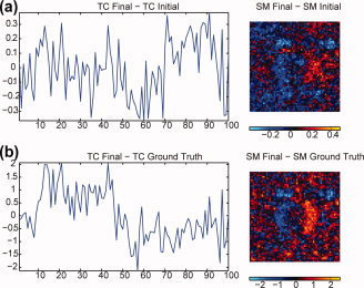
Iterating STR until convergence changes the estimated TCs and SMs from the single‐iterate version. (a) The difference between the initial STR iterate and the resulting TC and SM upon convergence. (b) The difference of the converged TC and SM and the truth, compare to Figure 6b (SS ICA STR).

Figure 12.

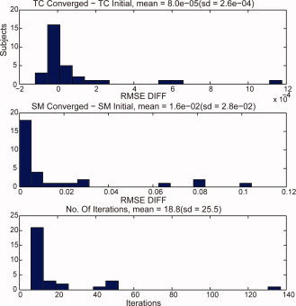
Iterating STR until convergence differences in RMSE with truth with iteration and with single iteration for TCs and SMs and number of iterations until convergence.

Auditory Oddball Task Data

GICA3 and STR method comparisons for real data is qualitative because we do not know the true TCs and SMs for the subjects. Analysis decisions and comparisons are guided by the results of the simulated data above. We select the default mode network (DMN) component because it a clear and prominent component previously identified [Calhoun et al.,2008a]. The subject‐level PCA reduces the data from 249 time points to T ₁ = 45 dimensions. We assume the estimation of the number of components by MDL is roughly correct, where the 28 subjects have a range from 11 to 26 estimated components with an average of 19, therefore we use T ₂ = 19 components for the group‐level PCA. Because subject‐specific and group data mean subject‐level PCA give very similar and good results, we choose subject‐specific to simplify the comparisons, and comparing the results from these two subject‐level PCA methods revealed minor differences that do not affect the results below. As suggested by the TC and SM estimation results in Figure 8, Figure 9, Figure 10, and Table II, ICA is better for GICA3 and PICA is better for STR, so we use these combinations so each method is at its best. Because we are using spatial ICA, we are more interested in differences in SMs than TCs between the GICA3 and STR methods.

For the AOD analysis, first we compare mean results for GICA3 and STR in Figure 13. Event‐related TC averages to the target stimulus for a task‐related (targets) component and the default mode network show that both GICA3 and STR provide similar results. In addition, the t statistics of the SMs for the default mode network appear similar for GICA3 and STR, apart from minor differences.

Figure 13.

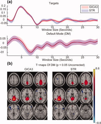
(a) AOD event‐related TC averages for the task‐related component and default mode network for GICA3 and STR. (b) Default mode network group t statistic SM for GICA3 and STR thresholded at uncorrected p‐value = 0.05.

For each subject, we calculate the Pearson correlation between the estimated SMs with GICA3 and STR and select the subjects with the highest and lowest correlations, representing the subjects estimated most similarly and most differently between the GICA3 and STR methods. We then z‐score and plot the TCs and SMs for these subjects for the two methods, as well as the differences in z‐score between the two methods. Note that the GICA3 and STR method correlation of a subject‐specific SM does not predict the correlation of the associated TC (not shown).

Figure 14 compares GICA3 and STR using the AOD data for the default mode network component in a similar format to Figure 7. Results for the subject‐specific TCs and SMs for two subjects are z‐scored and displayed in nine equally spaced axial slices from 60 mm to −20 mm, the SMs thresholded at 1.0 and the difference SMs thresholded at 0.5. Because the TCs are more complex for the real data, we concentrate on the SMs. We observe similar artifacts as in the simulated data from STR compared to GICA3. For the subject (24) with the highest inter‐method spatial correlation, the difference SM reveals bright red in slices 50 and −10 where STR has negative activation not appearing in GICA3. For the subject (21) with the lowest correlation, the difference SM reveals two important differences. First, GICA3 indicates more DMN activation with the red blobs in slices 50 through 20. Second, STR has a number of potential artifacts, spots of positive activation in slices 10 to −20 appearing as bright blue blobs in the difference map. Therefore, as in the simulated data, GICA3 suggests cleaner SMs with more activation where it is expected while STR includes more hypothesized artifacts.

Figure 14.

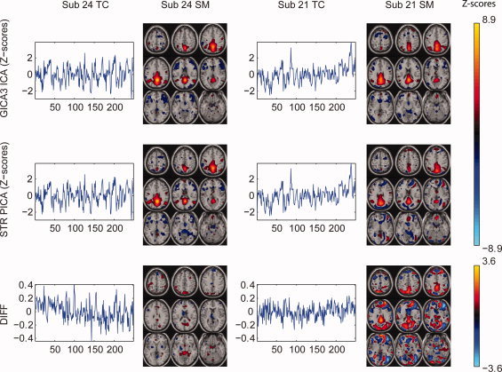
GICA3 and STR estimated z‐scored TCs, SMs, and differences for the most (24) and least (21) spatially correlated subjects between the two methods for AOD fMRI data, DMN component. SMs thresholded at 1.0 and the difference SMs thresholded at 0.5 displayed in nine equally spaced axial slices from 60 mm to −20 mm. Units are in standard deviations.

Simulated Resting‐State Data

For the resting‐state simulation we wished to determine the degree to which the PCA results in Figure 3 and the ICA back‐reconstruction results in Figure 4 were conditional on the task paradigm in Figure 2. Results (not shown) are qualitatively similar to what is observed in Figure 3 and Figure 4 suggesting our results are generalizable to many paradigms.

Simulated Demographic Data

We compared the ability of GICA3 and STR to detect spatial map intensities that depend on a covariate. Figure 15 shows the t statistics over the 100 subjects for testing whether the mean is zero for the three components with a covariate mask. Component 1 had binary and continuous masks around the left blob, Component 2 had continuous and interaction masks around the two upper blobs, and Component 3 had binary and interaction masks around the right blob. The Simulation rows are calculated from the “true” simulated SMs. The GICA3 and STR rows are calculated on the estimated SMs. GICA3 closely matches the Simulation while STR has many artifacts, either from the remaining component incorrectly appearing with the mask region or component mixing.

Figure 15.

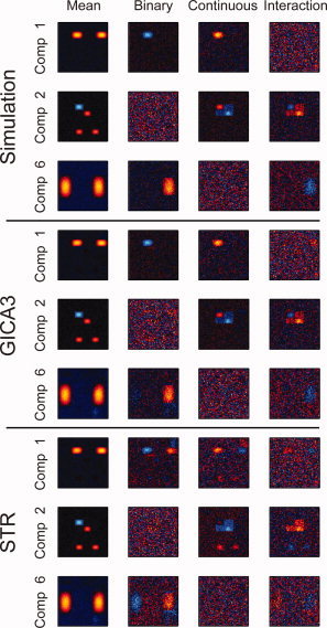
Unthresholded t statistics for “true” simulated SMs of demographic effects and GICA3 and STR t statistics to compare. More similar to the simulation is better.

Using the “true” simulated t statistics significant at an uncorrected 0.05 significance level as a mask, Table III compares the proportion of significant t statistics computed from GICA3 and STR agreeing with the “true” t statistics. The label “inside mask” is used to indicate the “true” t statistic was significant at a 0.05 significance level, and “outside mask” indicates insignificance. For the three effects (binary, continuous, and interaction) for the three components of interest when they had a simulated mask (Sim = Y), GICA3 usually has a greater proportion of voxels in agreement with the simulated t statistics than STR both inside and outside the mask. For the remaining components STR agrees more with the mask, but this is effectively agreement with random noise.

Table III.

Simulated demographic data, proportion of significant t statistics computed from GICA3 and STR agreeing with the “true” t statistics for the three components of interest

Component	Sim	Inside mask			Outside mask			Total
		Voxels	GICA3	STR	Voxels	GICA3	STR	GICA3	STR
Binary
1	Y	313	0.818	0.706	3,287	0.985	0.957	0.971	0.936
2	N	180	0.789	0.811	3,420	0.988	0.996	0.978	0.986
6	Y	458	0.745	0.478	3,142	0.970	0.922	0.941	0.865
Continuous
1	Y	275	0.811	0.567	3,325	0.987	0.984	0.973	0.952
2	Y	438	0.840	0.845	3,162	0.988	0.948	0.970	0.935
6	N	150	0.820	0.960	3,450	0.985	0.975	0.978	0.974
Interaction
1	N	166	0.717	0.831	3,434	0.986	0.971	0.974	0.965
2	Y	354	0.811	0.782	3,246	0.993	0.974	0.975	0.955
6	Y	298	0.638	0.540	3,302	0.983	0.979	0.955	0.943
	Binary total		Continuous total		Interaction total
Component	GICA3	STR	GICA3	STR	GICA3	STR
3	0.981	0.996	0.980	0.992	0.985	0.994
4	0.956	0.972	0.969	0.981	0.973	0.980
5	0.981	0.987	0.981	0.989	0.980	0.990
7	0.966	0.970	0.963	0.974	0.973	0.973
8	0.968	0.976	0.971	0.976	0.971	0.981

The label “inside mask” is used to indicate the “true” t statistic was significant at a 0.05 significance level, and “outside mask” indicates insignificance. Sim indicates a mask was applied to the component for the given covariate.

DISCUSSION

A detailed discussion follows a summary of the recommendations based on the mathematical results, model interpretations, and the PCA and ICA results. We recommend using standard PCA and noise‐free ICA because PPCA provides the same results as PCA and because PICA introduces artifacts into the estimated SM compared to ICA. We recommend using subject‐specific or group data mean subject‐level PCA because both provide similar TCs and SMs with accurate amplitude (see Table II, Figure 5 and Figure 6). We recommend retaining more components in the subject‐level PCA than in the group‐level PCA because back‐reconstruction results are better (see Figure 4). We recommend using GICA3 as the back‐reconstruction method because it is robust to the number of components retained for the group‐level PCA, because it provides the most accurately estimated TCs and SMs, because it has the desired interpretation of the product of TC and SM equal to the data to the accuracy of the PCA reduction, and because the aggregate SM is the sum of the well‐estimated subject‐specific SMs. The highly similar results for the simulations and real data suggest these recommendations apply for a wide variety of data.

PCA

We have shown that the subject‐specific and group data mean subject‐level PCA are preferred over spatial‐concatenation for a task‐paradigm data because the estimated TCs and SMs are less noisy and because TC scaling is poor with spatial concatenation (Table II, Figure 4, 5, 6, 4, Figure 5, Figure 6 and Figure 8). We recommend using subject‐specific PCA because group data mean is computationally intensive and because it gives similar results. We recommend retaining more components in the subject‐level PCA than at the group level, and preferably at least the maximum number of estimated components over all subjects, since this improves TC and SM estimation (see Figure 4). Subject‐specific PCA privileges subject differences at the subject‐level, while the group‐level PCA favors subject commonalities. Thus, the group‐level PCA is well informed by the full extent of variability in the subjects, and the subject‐specific information improves back‐reconstruction. As a practical note, we do acknowledge memory considerations can be a factor in justifying reducing the first level data as much as possible, however as we have shown that the trade‐off is slightly less accurate results.

The subject‐level PCA reduces the dimension of the problem to reduce computation memory and time. Additionally, the PCA rotation and dimension reduction often improves convergence of the ICA algorithm.

Subject Back‐Reconstruction Methods

The four methods (GICA1, GICA2, GICA3, and STR) are equivalent with no PCA reduction at the level of a single subject. The key difference between GICA3 and GICA1 is the partitioning of the group PCA matrix G, and GICA3 is preferred because it provides a natural interpretation for the subject‐specific TC and SM pairs. GICA2 does not use TCs and SMs from the same model (TC from GICA1 and SM from GICA3) which makes the fitted values not a projection, so GICA2 is not a preferred method. The GICA3 subject‐specific TCs and SMs all derive directly from the PCA and ICA, while STR uses only the aggregate SM from the ICA and relies on the contradictory assumptions of a common SM and then distinct subject‐specific SMs in the two least‐squares regression steps.

GICA3 has two desirable properties. First, the product of the subject‐specific TCs and SMs predict the subject data to the accuracy of information retained from PCA, . Second, the sum of the subject‐specific SMs is the aggregate ICA SM, which is analogous to a random effects model where the subject‐specific effects are zero‐mean distributed deviations from the group mean effect. Additionally, because subject‐specific SMs are more accurately estimated by GICA3 than STR, inference of group spatial activation differences, for example, are also expected to be more accurate using GICA3.

STR is similar to GICA1 to the level of PCA reduction. The first regression using the STR method from (19) gives Ṙ _i = Y _i Ŝ ⁻, and GICA1 from (17) gives R̂ _i = F _i G _i  ≈ Y _i Ŝ ⁻. Thus Ṙ _i ≈ R̂ _i, the subject‐specific TC from STR and GICA1 are similar, with similarity increasing with the information retained by the PCA steps F _i and G, and equivalent with no PCA reduction. The second regression using the STR method from (21) gives Ṡ _i = Ṙ ${}_{\mathit{\text{i}}}^{\text{−}}$ Y _i, and substituting the equivalent estimate from GICA1, we have Ṡ _i = Ṙ ${}_{\mathit{\text{i}}}^{\text{−}}$ Y _i ≈ R̂ ${}_{\text{−}}^{\mathit{\text{i}}}$ Y _i. Thus Ṡ _i ≈ Ŝ _i, the subject‐specific SM using STR and GICA1 are similar, and equivalent with no PCA reduction (see Figure 4 and Figure 8–Figure 10).

Three criticisms of STR follow. STR initially assumes a common SM for all individuals to estimate subject‐specific TCs in (19), then estimates subject‐specific SMs given the TCs in (21), thus the original common SM assumption and the later estimated SMs present a contradiction. From (21) it is unclear how to interpret the subject‐specific SMs since they are the product of the aggregate SM and a rank‐deficient approximation to an identity matrix based on the subject data. The relationship between the subject SMs and aggregate SM in (23) is difficult to interpret, that is, it is not straightforward as in GICA3 near (12).

In the poster introduction of STR [Beckmann et al.,2009], a number of claims were made which this article clearly refutes by a comprehensive study. First, regarding the claim that when using GICA methodology the “final statistical comparison on the back‐projected maps can lead to significant inaccuracies,” we have shown that the most accurate SMs are those provided by GICA3 (see Figure 8–Figure 10). Second, in [Beckmann et al.,2009], there is a comparison of STR and GICA2 where, though 10 components were simulated, only five components were purposefully retained for analysis. In this case, as stated by the same authors in a previous article, “underestimation of the dimensionality will discard valuable information and result in suboptimal signal extraction” [Beckmann and Smith,2004]. The correct number of components should be retained, or at least an estimate of the correct number of components, though in practice one does not know what that number is and it may differ between subjects. Third, there is a claim that STR can estimate global amplitude differences while GICA cannot. In fact, it is the spatial concatenation subject‐level PCA [Beckmann et al.,2005] that can influence amplitude, not the back‐reconstruction methods which all retain amplitude information. As an aside, GIFT software, has a “calibrate” option to scale to percent signal change that works with the GICA methods and STR.

Finally, one can think about predicting subject data based on a fitted model to the aggregate SM. Both GICA1 and GICA3 predict the subject data as the product of the TC and SM, Ŷ _i = R̂ _i Ŝ _i = R̃ _i S̃ _i = P ${}_{\mathit{\text{C}}\text{(}\mathbf{\text{F}}{}_{\mathit{\text{i}}}\mathbf{\text{G}}{}_{\mathit{\text{i}}}\text{)}}$ Y _i. From ICA (6) we have X = Â Ŝ, and we can use the aggregate SM Ŝ to fit the subject‐specific data. Using GICA1 we have , and GICA3 in (30) we have , where both fitted values are the same, , so both are in C(F _i G _i). For GICA1 (or GICA3) the columns of R̂ _i (or R̃ _i) define a basis for C(F _i G _i) and Ŝ _i (or S̃ _i) provide the coordinates of in that basis. The observed data Y _i, the GICA1 (or GICA3) fitted value Ŷ _i (or Ỹ _i), and the aggregate fitted value (or ) relate to each other,

(29)

The first term on the right‐hand side, (Y _i − Ŷ _i)^T(Y _I − Ŷ _i), is the residual sum of squares between the data and the GICA1 (or GICA3) fitted value with (Y _i − Ŷ _i) ∈ C(F _i G _i)^⟂, the orthogonal complement of C(F _i G _i). The second term on the right‐hand side, , is the between‐subject sum of squares, with . Thus, the “closer” Ŷ _i is to , the “closer” Ŝ _i is to Ŝ. Hence, one can think of GICA1 (or GICA3) as finding an optimal Ŝ _i (or S̃ _i) such that Ŷ _i (or Ỹ _i) lies in the same subspace as (or ).

CONCLUSION

Multi‐subject ICA approaches are becoming more widely used, but they can vary in how the data reduction and ICA steps are implemented. There has been little work done to carefully evaluate the properties of these different approaches and the impact on the results. In this work, we performed extensive analyses on simulated and real data to provide guidelines regarding the various approaches. Of the methods we evaluated, evidence suggests that noise‐free PCA with noise‐free ICA with back‐reconstruction method GICA3 provides the most robust results with the most intuitive/natural interpretation.

This appendix derives or illustrates the relationships mentioned in the text.

Subject Back‐Reconstruction Methods

GICA3

The product of each subject‐specific TC and SM is a perpendicular projection of the data onto the PCA column space,

(30)

Fitted values and data agree in the PCA space,

(31)

The fitted compressed values, , are a product of the subject‐specific TC and SM,

(32)

and similarly for the mean fitted compressed value,

(33)

STR

The product of each subject‐specific TC and SM gives Ṙ _i Ṡ _i = Ṙ _i(Ṙ ${}_{\text{T}}^{\mathit{\text{i}}}$ Ṙ _i)⁻¹ Ṙ ${}_{\text{T}}^{\mathit{\text{i}}}$ Y _i = P ${}_{\mathit{\text{C}}\text{(}\mathbf{\text{Ṙ}}{}_{\mathit{\text{i}}}\text{)}}$ Y _i = P ${}_{\mathit{\text{C}}\text{(}\mathbf{\text{Y}}{}_{\mathit{\text{i}}}\mathbf{\text{Ŝ}}{}^{\text{−}}\text{)}}$ Y _i where P ${}_{\mathit{\text{C}}\text{(}\mathbf{\text{Ṙ}}{}_{\mathit{\text{i}}}\text{)}}$ = P ${}_{\mathit{\text{C}}\text{(}\mathbf{\text{Y}}{}_{\mathit{\text{i}}}\mathbf{\text{Ŝ}}{}^{\text{−}}\text{)}}$ is a PPO onto C(Y _i Ŝ ⁻), which is not an intuitive column space,

(34)

REFERENCES

- Attias H ( 1999): Independent factor analysis. Neural Computation 11: 803–851. [DOI] [PubMed] [Google Scholar]
- Bartholomew DJ, Knott M ( 1987): Latent Variable Models and Factor Analysis. Griffin London. [Google Scholar]
- Basilevsky A ( 1994): Statistical Factor Analysis and Related Methods: Theory and Applications. New York: Wiley. [Google Scholar]
- Beckmann CF, DeLuca M, Devlin JT, Smith SM ( 2005): Investigations into resting‐state connectivity using independent component analysis. Phil Trans R Soc B 360: 1001–1013. [DOI] [PMC free article] [PubMed] [Google Scholar]
- Beckmann CF, Mackay CE, Filippini N, Smith SM ( 2009): Group comparison of resting‐state fMRI data using multi‐subject ICA and dual regression. FMRIB Centre, Dept. of Clinical Neurology, University of Oxford, Oxford, United Kingdom: Available at: http://www.humanbrainmapping.org/files/HBM2009OnsiteProgram-Final.pdf. [Google Scholar]
- Beckmann CF, Smith SM ( 2003): Probabilistic ICA for FMRI—Noise and Inference, 4th International Symposium on Independent Component Analysis and Blind Signal Separation (ICA2003), April 2003, Nara, Japan. 295–300.
- Beckmann CF, Smith SM ( 2004): Probabilistic independent component analysis for functional magnetic resonance imaging. IEEE Trans Med Imaging 23: 137–152. [DOI] [PubMed] [Google Scholar]
- Beckmann CF, Smith SM ( 2005): Tensorial extensions of independent component analysis for multisubject FMRI analysis. NeuroImage 25: 294–311. [DOI] [PubMed] [Google Scholar]
- Calhoun VD ( 2004): Group ICA of fMRI toolbox (GIFT). Available at: http://icatb.sourceforge.net.
- Calhoun VD, Adali T, McGinty V, Pekar JJ, Watson T, Pearlson GD ( 2001a): fMRI activation in a visual‐perception task: Network of areas detected using the general linear model and independent component analysis. NeuroImage 14: 1080–1088. [DOI] [PubMed] [Google Scholar]
- Calhoun VD, Adali T, Pearlson GD, Pekar JJ ( 2001b): A method for making group inferences from functional MRI data using independent component analysis. Human Brain Mapping 14: 140–151. [DOI] [PMC free article] [PubMed] [Google Scholar]
- Calhoun VD, Adali T, Pearlson GD, Pekar JJ ( 2002): Erratum: A method for making group inferences from functional MRI data using independent component analysis. Human Brain Mapping 16: 131. [DOI] [PMC free article] [PubMed] [Google Scholar]
- Calhoun VD, Adali T, Pekar JJ ( 2004a): A method for testing conjunctive and subtractive hypotheses on group fMRI data using independent component analysis. Magn Reson Imag 22: 1181–1191. [DOI] [PubMed] [Google Scholar]
- Calhoun VD, Pekar JJ, Pearlson GD ( 2004b): Alcohol intoxication effects on simulated driving: Exploring alcohol‐dose effects on brain activation using functional MRI. Neuropsychopharmacology 29: 2097–2107. [DOI] [PubMed] [Google Scholar]
- Calhoun VD, Kiehl KA, Pearlson GD ( 2008a): Modulation of temporally coherent brain networks estimated using ICA at rest and during cognitive tasks. Human Brain Mapping 29: 828–838. [DOI] [PMC free article] [PubMed] [Google Scholar]
- Calhoun VD, Pearlson GD, Maciejewski P, Kiehl KA ( 2008b): Temporal lobe and "default" hemodynamic brain modes discriminate between schizophrenia and bipolar disorder. Hum Brain Map 29: 1265–1275. [DOI] [PMC free article] [PubMed] [Google Scholar]
- Calhoun VD, Liu J, Adal T ( 2009): A review of group ICA for fMRI data and ICA for joint inference of imaging, genetic, and ERP data. NeuroImage 45: 163–172. [DOI] [PMC free article] [PubMed] [Google Scholar]
- Celone KA, Calhoun VD, Dickerson BC, Atri A, Chua EF, Miller S, DePeau K, Rentz DM, Selkoe D, Albert MS ( 2006): Alterations in memory networks in mild cognitive impairment and Alzheimer's disease: An independent component analysis. J Neurosci 26: 10222–10231. [DOI] [PMC free article] [PubMed] [Google Scholar]
- Correa N, AdalI T, Calhoun VD ( 2007): Performance of blind source separation algorithms for fMRI analysis using a group ICA method. Magn Reson Imag 25: 684–694. [DOI] [PMC free article] [PubMed] [Google Scholar]
- Davies M ( 2004): Identifiability issues in noisy ICA. IEEE Signal Proc Lett 11: 470–473. [Google Scholar]
- De Lathauwer L, De Moor B, Vandewalle J ( 1996): A technique for higher‐order‐only blind source separation. Proc. of the International Conference on Neural Information Processing (ICONIP'96), Hong Kong, China, Sept. 1996. pp 1223–1228.
- Esposito F, Scarabino T, Hyvarinen A, Himberg J, Formisano E, Comani S, Tedeschi G, Goebel R, Seifritz E, Di SF ( 2005): Independent component analysis of fMRI group studies by self‐organizing clustering. Neuroimage 25: 193–205. [DOI] [PubMed] [Google Scholar]
- Guo Y, Pagnoni G ( 2008): A unified framework for group independent component analysis for multi‐subject fMRI data. NeuroImage 42: 1078–1093. [DOI] [PMC free article] [PubMed] [Google Scholar]
- Himberg J, Hyvärinen A, Esposito F ( 2004): Validating the independent components of neuroimaging time series via clustering and visualization. NeuroImage 22: 1214–1222. [DOI] [PubMed] [Google Scholar]
- Hyvärinen A ( 1999a): Fast ICA for noisy data using Gaussian moments. Circuits and Systems, 1999. ISCAS '99. Proceedings of the 1999 IEEE International Symposium on, vol. 5, no., pp. 57–61 vol. 5, 1999. Available at: http://ieeexplore.ieee.org/stamp/stamp.jsp?tp=&arnumber=777510&isnumber=16880
- Hyvärinen A ( 1999b): Gaussian moments for noisy independent component analysis. IEEE Signal Proc Lett 6: 145–147. [Google Scholar]
- Hyvärinen A, Karhunen J, Oja E ( 2001): Independent Component Analysis, Adaptive and Learning Systems for Signal Processing, Communications, and Control. New York: John Wiley & Sons. [Google Scholar]
- Kiehl KA, Laurens KR, Duty TL, Forster BB, Liddle PF ( 2001): Neural sources involved in auditory target detection and novelty processing: An event‐related fMRI study. Psychophysiology 38: 133–142. [PubMed] [Google Scholar]
- Kiehl KA, Stevens MC, Laurens KR, Pearlson G, Calhoun VD, Liddle PF ( 2005): An adaptive reflexive processing model of neurocognitive function: Supporting evidence from a large scale (n = 100) fMRI study of an auditory oddball task. NeuroImage 25: 899–915. [DOI] [PubMed] [Google Scholar]
- Li YO, Adali T, Calhoun VD ( 2007): Estimating the number of independent components for functional magnetic resonance imaging data. Human Brain Mapping 28: 1251–1266. [DOI] [PMC free article] [PubMed] [Google Scholar]
- Lukic AS, Wernick MN, Hansen LK, Strother SC ( 2002): An ICA Algorithm for Analyzing Multiple Data Sets. Image Processing. 2002. Proceedings. 2002 International Conference on, vol. 2, no., pp. II‐821–II‐824 vol. 2, 2002. Available at: http://ieeexplore.ieee.org/stamp/stamp.jsp?tp=&arnumber=1040077&isnumber=22295.
- Moulines E, Cardoso JF, Gassiat E ( 1997): Maximum likelihood for blind separation and deconvolution of noisy signals using mixture models. Acoustics, Speech, and Signal Processing, 1997. ICASSP‐97, 1997 IEEE International Conference on, vol. 5, no., pp. 3617–3620 vol. 5, 21–24 Apr 1997. Available at: http://ieeexplore.ieee.org/stamp/stamp.jsp?tp=&arnumber=604649&isnumber=13273
- Okada T, Yamada H, Ito H, Yonekura Y, Sadato N ( 2005): Magnetic field strength increase yields significantly greater contrast‐to‐noise ratio increase: Measured using BOLD contrast in the primary visual area1. Acad Radiol 12: 142–147. [DOI] [PubMed] [Google Scholar]
- Pearson K ( 1901): LIII. On lines and planes of closest fit to systems of points in space. Philos Mag Ser 6 2: 559–572. [Google Scholar]
- Schmithorst VJ, Holland SK ( 2004): Comparison of three methods for generating group statistical inferences from independent component analysis of functional magnetic resonance imaging data. J Magn Reson Imag 19: 365–368. [DOI] [PMC free article] [PubMed] [Google Scholar]
- Svensén M, Kruggel F, Benali H ( 2002): ICA of fMRI group study data. NeuroImage 16( 3PA): 551–563. [DOI] [PubMed] [Google Scholar]
- Tipping ME, Bishop CM ( 1999): Probabilistic principal component analysis. J Royal Stat Soc Ser B (Statistical Methodology) 61: 611–622. [Google Scholar]
- Varoquaux G, Sadaghiani S, Pinel P, Kleinschmidt JB, Poline JB, Thirion B ( 2010): A group model for stable multi‐subject ICA on fMRI datasets. NeuroImage 51: 288–299. [DOI] [PubMed] [Google Scholar]