

Abstract
The bacterial flagellum is a self-assembling filament, which bacteria use for swimming. It is built from tens of thousands of flagellin monomers in a self-assembly process that involves translocation of the monomers through the flagellar interior, a channel, to the growing tip. Flagellum monomers are pumped into the filament at the base, move unfolded along the channel and then bind to the tip of the filament, thereby extending the growing flagellum. The flagellin translocation process, due to the flagellum maximum length of 20 μm, is an extreme example of protein transport through channels. Here, we derive a model for flagellin transport through the long confining channel, testing the key assumptions of the model through molecular dynamics simulations that also furnish system parameters needed for quantitative description. Together, mathematical model and molecular dynamics simulations explain why the growth rate of flagellar filaments decays exponentially with filament length and why flagellum growth ceases at a certain maximum length.
Introduction
In many living systems, proteins need to be transported from where they are synthesized to where they are needed. Protein transport often requires unfolded proteins to pass through narrow pores or channels. Examples of protein transport systems are SecY (1) or the mitochondrial translocase of outer membrane and translocase of inner membrane (2). Translocation can be driven by passive diffusion (3) or by active, i.e., energy-consuming, transport (4). Much theoretical research has focused on protein translocation through pores (3,5–8) and channels (9,10). The bacterial flagellum, which allows bacteria to propel themselves (11–14), is a unique class of protein transport systems in that the conducting channel is considerably longer than the translocated protein (15).
The flagellar filament is typically L = 10–20 μm long and is built from tens of thousands of flagellin monomers stacked in a helical pattern leaving an interior space, the channel, as shown in Fig. 1 (16,17). Each repeat of the helix involves 11 monomers and a rise of 52 Å. The flagellin protein, Protein Data Bank code 1UCU (17), consists of 494 amino acids. Fig. 1 shows the structure of the four flagellin domains, D0 (residues 1–55, 451–494), D1 (residues 56–176, 402–450), D2 (residues 177–189, 284–401), and D3 (residues 190–283) (17–19). CD0 (residues 457–494) is an α-helix at the C-terminus, which comprises the inner surface of the filament channel that has a radius of Å (17).
Figure 1.
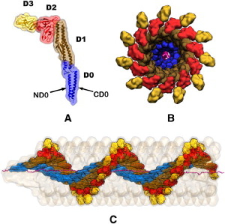
Flagellum structure. The flagellum is built from flagellin monomers stacked in a helical pattern. (A) The folded flagellin consists of four domains: D0 (blue), D1 (brown), D2 (red), and D3 (gold). (B) View along the filament axis shows how the domains are ordered by their distance from the channel's center. D0 is the inward most domain. CD0 is the α-helix at the C-terminus of the D0 domain; it comprises the channel's inner surface. (C) Side view, with most of the filament monomers removed, shows how an unfolded flagellin monomer (magenta) spreads through the filament channel at near-maximal extension.
The flagellum is a self-assembling system. In the basal body, which anchors the rotating flagellum to the cell membrane (20), a type III secretion system pumps newly synthesized, unfolded, flagellin monomers into the flagellum channel (21–25). Each added monomer displaces its distal neighbor toward the tip of the filament, the secretion pump providing the driving force to translocate all flagellins in the channel toward the growing tip. The flagellin monomers translocate in an unfolded conformation through the filament to the distal end of the flagellum, where they fold into an active conformation and bind to the filament with the help of a cap protein, thereby extending the flagellum (26). Though both flagellum and translocating protein are comprised of flagellin, the term “flagellin” will be used here to denote only the translocating, unfolded, protein.
Regarding flagellum growth, Iino (16) demonstrated that the rate of filament elongation in vivo decays exponentially with length, whereas the growth rate in vitro (allowing flagellin in bulk water to bind directly to the flagellum tip without traversing the flagellum) is constant. The in vivo decrease in rate was shown to result from a decrease in translocation efficiency as the filament grows. Levy (27,28) sought to describe the flagellum growth rate in terms of a concentration gradient of a flagellar binding factor. This model, developed before the channel structure had been solved (13), was based on the assumption that flagellin could freely diffuse from the base to the tip and did not correctly reproduce the exponential decay in the growth rate (16). We explain the observed filament growth rate and its length-dependence in terms of the molecular properties of unfolded, i.e., translocating, flagellin and of folded flagellin, helically assembled into a flagellum.
A straightforward approach to the intended study might be an all-atom simulation of translocating flagellin and the elongating filament; however, the large size of the flagellum and the long timescale of growth render this approach intractable. The authors, rather, adopt a strategy, which starts from a mathematical model of the translocation-elongation process; the model describes all properties influencing the process rate, including flagellin density, compressibility, and friction, and reproduces the observation reported in Iino (16) as well as overall filament length. The local physical properties underlying the model are then verified through molecular dynamics simulations, the model thus furnishing a bridge between small molecule-short timescale properties of the translocating flagellin accessible to molecular dynamics and the large size-long time behavior of the growing flagellum accessible to experiment (16).
Below, we present the theoretical description of flagellin translocation, which includes several assumptions that are either assumed self-evident or verified through simulation. Next, we outline the molecular dynamics simulations employed to verify the assumptions made and to furnish key system parameters needed to calculate the flagellum growth rate.
Methods
Our mathematical description of flagellin translocation is based on a minimum set of rather self-evident assumptions and on certain mechanical properties. The model is shown to agree well with observed growth rates, in particular, their length dependence. Molecular dynamics simulations carried out to test the relationship between model and molecular characteristics are then described.
Theory of flagellin translocation and flagellum growth
Our description of translocating unfolded flagellin is based on five position-dependent properties. These properties depend on their distance from the channel tip, x, and on the length of the flagellum, L. We emphasize that x denotes the distance from the tip, not from the base. The five characteristics are:
-
1.
Flagellin density, ρ(x, L) (in units flagellin/volume).
-
2.
Flagellin pressure, p(x, L) (in units force/area).
-
3.
Friction density, g(x, L) (in units force/area). Note that the friction is due to atomic interactions at the contact surface between flagellin and channel.
-
4.
Flagellin flux, ϕ(x, L) (in units flagellin/(time × area)).
-
5.
Translocation velocity, v(x, L) (in units length/time).
The theoretical description begins with a derivation of flagellin pressure, p(x, L). It then uses this expression to derive expressions for the remaining four flagellin properties. Finally, the flagellum growth rate is calculated from these properties. The derivation is based on several conditions, which the translocating flagellin system must meet for the model to apply. These conditions are stated and are either argued to be self-evident or are verified through molecular dynamics simulations.
We start by postulating
Condition 1: Flagellin pressure, p, is isotropic.
The radial pressure which unfolded flagellin exerts against the channel surface should be equal to the axial pressure which it exerts on its proximal and distal neighbors,
| (1) |
Indeed, we expect that a denatured protein, a self-avoiding but otherwise rather flexible polymer, possesses this property typical for a fluid and does relay compression exerted on it both axially and radially.
The next two postulates,
Condition 2: Friction density, g, is proportional to flagellin pressure, p,
and
Condition 3: Translocating flagellin is in mechanical equilibrium,
are closely related and rely on the fact that the maximum translocation velocity in the flagellar channel is ∼1 nm/ms, whereas the maximum growth rate, V0, is ∼0.1 Å/ms (16); this slow velocity is central to the behavior of friction between a flagellin and the channel. For velocities below a critical velocity, vc (typically ∼1 nm/ms), friction is not characterized by a velocity-dependent dynamic friction, but rather by velocity-independent static friction (29,30), known as “creeping” static friction (31,32). Because of the small driving forces and slow translocation rates present in the flagellum, flagellar friction is due to creeping static friction (33).
The flagellin-channel friction manifests itself through resistance to lateral (along channel axis) force which, over a segment [x + dx, x], is due to the pressure difference at x + dx and x and measures . The resisting force, creeping static friction, is due to adhesion of flagellin to the channel surface, 2πRdx, and is stated in the form , where g(x, L) is the static friction per unit contact area. Both channel surface and translocating flagellin are fluctuating conformationally, such that adhesion interactions are constantly formed and broken; as a result flateral imposes a bias that the flagellin reforms its contacts with the channel further toward the distal tip; fresistance arises from the number of adhesion spots averaged along the channel and through time. This average is proportional to the number of flagellin surface atoms pressing against the channel wall and, hence, is proportional to the isotropic pressure of flagellin.
Because translocation is so slow, Condition 2 cannot be tested through simulation. However, we demonstrate below that in the pressure and density ranges relevant for flagellin transport, pressure and surface contact density (number of contacts exposed to channel surface per unit surface area), namely Ncontact/Acontact, are linearly related as
| (2) |
We express Condition 2 through
| (3) |
where α is a dimensionless proportionality coefficient, and Condition 3 through
| (4) |
For dx → 0, this reads
| (5) |
Equations 3 and 5 combine to the differential equation
| (6) |
the solution of which is
| (7) |
In Eq. 7, p0(L) is the flagellin pressure at the tip of the flagellum that pushes flagellin against the cap protein and is controlled through the nonzero force, ftip (26), with which the cap protein resists flagellin to pass through the tip, such that the condition
| (8) |
holds. Accordingly, we assume
Condition 4: Flagellin pressure at the flagellar tip is ftip/πR2.
Equation 8 implies that p(x, L) is L-independent, namely
| (9) |
Fig. S1 in the Supporting Material plots p(x) for the flagellum. Equation 9, combined with Eq. 3, now yields an expression for friction density,
| (10) |
A crucial property controlling translocation in the flagellar channel is the isothermal compressibility, κT, of the translocated flagellin. For a given relationship between exerted pressure and flagellin density, the compressibility is , where V = Nρ−1. If the flagellin atoms were disconnected, as noninteracting point particles, the ideal gas law would hold, namely, p = kBT ρ. This pressure-density relationship is clearly an oversimplification. A more realistic description represents flagellin as a so-called Gaussian chain (34,35). In the case of this simple polymer model holds approximately the relationship
| (11) |
as we demonstrate in the Supporting Material. Here b is the so-called effective bond length for a Gaussian chain (b equals two times the polymer persistence length lp (35)), L0 the length of the polymer chain when it is totally stretched, and the density of one polymer chain, defined through the polymer atom density/number of the atoms in a single polymer. One can see from Eq. 11 and the Supporting Material that for increasing holds with β = 3. In this case holds κT = 1/βp. In a more realistic description, the actual exponent β should differ from β = 3 due to atomic interactions that are neglected in the Gaussian chain model (34). Accordingly, we stipulate
Condition 5: Flagellin pressure is a power of flagellin density.
Namely,
| (12) |
where ρ0 = 1 atom/Å3 is a reference density.
According to Eqs. 9 and 12, flagellin density can now be expressed as
| (13) |
Fig. S2 plots ρ(x) for the flagellum. The flagellin flux, ϕ, is the product of flagellin density, ρ, and translocation velocity, v,
| (14) |
For the density of flagellin in the channel to be stationary (time-independent), protein flux must be independent of x. Equation 14, therefore, simplifies to
| (15) |
This expression is most readily evaluated at x = L; for the evaluation, we assume
Condition 6: Flagellin monomers are pumped into the channel at a constant power, P.
The pump power, P, equals the product of pressure, cross-sectional area, and translocation velocity at x = L, i.e., , which can be written
| (16) |
Equation 15, combined with v(x,L)|x=L from Eq. 16, ρ(x)|x=L from Eq. 13 and p(x)|x=L from Eq. 9, becomes
| (17) |
where
| (18) |
Finally, one can substitute ϕ(L) from Eq. 17 and ρ(x) from Eq. 13 into Eq. 15 and obtain
| (19) |
Fig. S3 shows v(x, L) for the flagellum.
Rate of flagellin translocation and flagellum growth
We can now express the growth velocity of the flagellum, V(L) (in units length/time), as the product of the frequency with which flagellin monomers reach the tip, πR2ϕ(L) and the length which each flagellin contributes to L, λ = 5 Å/flagellin, namely
| (20) |
which, by substituting ϕ(L) from Eq. 17, becomes
| (21) |
where
| (22) |
and
| (23) |
For β → 1, the decay length, a, becomes infinite and, therefore, the growth rate would be constant such that V(L) = V0 holds in contrast to observation (16); thus, it is essential that β > 1 be established.
By defining the growth rate as the change in length with respect to time, i.e., V = dL(t)/dt, Eq. 21 can be integrated to express flagellum length as a function of time,
| (24) |
the solution of which, for , is
| (25) |
Fig. S4 presents L(t) for the flagellum.
This concludes the derivation of expressions for length, growth rate, and the five flagellin translocation properties. These expressions offer a wealth of insight into flagellin translocation through the long, confining flagellar channel and why the growth rate decays exponentially with length. Equation 13 states that, as the flagellum grows, flagellin density at the base increases. As a result, friction at the base grows (refer to Eq. 10). Increasing friction causes pressure to increase at the base (refer to Eq. 9). Because the secretion system operates at constant power, the increasing pressure required to pump in flagellin at the base means that the rate of insertion must decrease proportionally, thereby slowing the rate of translocation and, consequently, filament growth.
According to Eq. 25, the flagellum can grow infinitely long. What, then, halts the flagellum's growth at Lmax = 20 μm (16)? The answer is that even though the pump at the base of the filament operates at a constant power P, its force cannot increase indefinitely. In fact, when the pump reaches its stall force, fstall, filament elongation ceases, namely (refer to Eq. 9)
| (26) |
From this follows
| (27) |
The result shows that the maximum length of a flagellum can be extended by either increasing the ratio fstall/ftip, or by decreasing the coefficient of friction, α, defined in Eq. 3. Due to the weak, namely only logarithmic, dependence on fstall/ftip, α is the primary control of Lmax.
Verification of flagellin translocation model
Below, Conditions 1 and 5 are verified for the flagellum through molecular dynamics simulations. It will be demonstrated how compressing flagellin in a cylinder allows one to measure the needed physical characteristics as a function of flagellin density. Conditions 2 and 3 are assumed to hold true for the flagellum because the translocation velocity is extremely slow compared to the relaxation processes during translocation. Condition 2 relies on theoretical arguments given above, the key one being a linear relationship between pressure and the average number of adhesion points as stated by Eq. 2. Certainly, the linearity stated in Eq. 3 can hold only over a limited pressure interval, but should hold for the low pressures as they arise in flagellar transport. This will be demonstrated below. Condition 6 is evident for biological pumps, which operate by ATP hydrolysis at some fixed rate and have been shown to slow down under increasing load (36,37).
Simulations Carried Out
Molecular dynamics simulation methods
Ten nonequilibrium all-atom molecular dynamics simulations were performed (see Table 1) to study flagellin translocation and verify the conditions underlying our theoretical description. The first nine simulations involve a segment of unfolded flagellin being compressed in a cylinder (see Fig. 2); the 10th simulation is for a segment of flagellin translocated through the actual flagellar channel (see Fig. 3). We carried out also 60 simulations of a flagellin segment equilibrating in implicit solvent while confined to cylinders of different, but fixed, lengths and radii. Simulations were prepared and analyzed using VMD (38) and carried out with NAMD (39).
Table 1.
Simulations performed
| Name | Type | Residues | Channel | Atoms | Time |
|---|---|---|---|---|---|
| 5A | Comp. | 1–164 | 5 Å cyl. | 23,232 | 10 ns |
| 5B | Comp. | 165–329 | 5 Å cyl. | 23,142 | 10 ns |
| 5C | Comp. | 330–494 | 5 Å cyl. | 24,988 | 10 ns |
| 7A | Comp. | 1–164 | 7 Å cyl. | 31,811 | 10 ns |
| 7B | Comp. | 165–329 | 7 Å cyl. | 32,721 | 10 ns |
| 7C | Comp. | 330–494 | 7 Å cyl. | 33,800 | 10 ns |
| 9A | Comp. | 1–164 | 9 Å cyl. | 34,186 | 10 ns |
| 9B | Comp. | 165–329 | 9 Å cyl. | 32,077 | 10 ns |
| 9C | Comp. | 330–494 | 9 Å cyl. | 31,787 | 10 ns |
| CD0 | Trans. | 1–100 | CD0 | 69,664 | 52 ns |
| Equil. | Equil. | 1–164 | 60 cyls. | 2445 | 447 ns |
The first nine (Comp.) are simulations of unfolded flagellin being compressed in a cylinder (cyl.). The 10th simulation (Trans.) models flagellin translocation through the flagellum channel. The Equil. group of 60 simulations equilibrate flagellin segment A in cylinders of different geometries; these simulations employed an implicit solvent description.
Figure 2.
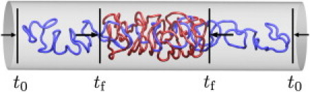
Flagellin compression simulation. To study the effects of confinement and density on translocation, three denatured flagellin segments, A, B, and C, were compressed in cylinders of radii 5, 7, and 9 Å. The piston walls (shown as black vertical lines) were moved toward each other from time t0 (flagellin backbone in blue) to time tf (flagellin backbone in red) at a velocity of 10 Å/ns. (Arrows) Piston force.
Figure 3.
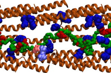
Flagellin translocation simulation. To simulate flagellin translocation through the flagellum, flagellin was pushed 52 Å through a channel lined by the CD0 domain (light brown). The repeating arginine residues of the CD0 domains are shown (dark blue); the acidic and basic residues of the translocated flagellin are also shown (dark red and dark blue, respectively). One of several transient salt bridges is shown with the interacting acidic and basic residues (colored light red and light blue, respectively).
In each simulation, temperature was held at 300 K by a Langevin thermostat, and a pressure of 1 atm was maintained by a Nosé-Hoover Langevin-piston barostat with a period of 200 fs and a decay rate of 300 fs; periodic boundary conditions were assumed. Multiple time stepping was employed using an integration timestep of 1 fs, with short-range forces evaluated every two timesteps and long-range electrostatic forces every four timesteps. The short-range forces were smoothed with a cutoff between 10 and 12 Å, while long-range electrostatic interactions were calculated using the particle-mesh Ewald algorithm. All simulations used the CHARMM22 (40) force field together with the TIP3P water model (41). A salt strength of 200 mM KCl was assumed to neutralize the charge of the system and in keeping with experiment (16). The structure for flagellin monomers of Salmonella typhimurium was obtained from the Protein Data Bank (code 1UCU (17)). The structure of the flagellar filament was solved by Yonekura et al. (13,17) and others (18,19,42).
Flagellin preparation
Flagellin was unfolded by fixing the N-terminal residue and pulling the C-terminal residue by steered molecular dynamics (43) in vacuum to a linear density of 0.25 residues/Å. Once stretched, the monomer was divided into three segments of equal length for the purpose of accelerated independent sampling: segment A with residues 1–164, segment B with residues 165–329, and segment C with residues 330–494. Copies of each stretched segment contracted and then equilibrated for 3 ns in a periodic water box while confined to cylinders of three different radii, namely 5, 7, and 9 Å, making nine segments, labeled 5A–9C, as listed in Table 1. Confinement to cylinders, achieved computationally through a Tcl force (39) (an external, user-specified force), involved a radial force f = −k × max(r − rc,0) to the backbone atoms, where r is the atom's distance from the cylinder axis and rc is the cylinder radius; for k we assumed a value 10 (kcal/mol)/Å2.
Compression
The flagellin segments, still confined to their respective radii, were axially compressed by another Tcl force (39), on the right side by f = −k × max(x − xc,0), and on the left side by f = −k × min(x + xc,0), where x is the atom's x coordinate (along the axis of the cylinder) and ±xc is the position of the right and left compression walls (shown as vertical lines in Fig. 2). The walls move inward as the compression progresses according to xc = x0 – vt, where x0 = 120 Å is the initial position of the compression walls, v = 10 Å/ns is the velocity at which the compression walls move inward, and t is the simulation time; one simulated system is illustrated in Fig. 2. Axial and radial pressure were calculated as the force exerted by the cylinder's two axial walls and radial wall on the protein, respectively, divided by their respective areas. Density was calculated as the number of protein atoms divided by the cylinder's changing volume.
Equilibration
To test the relationship between axial and radial pressure and density at equilibrium, flagellin segment A was equilibrated in cylinders of several lengths (L = 150, 165, 180, 195, 210, 225 Å) and radii (R = 5, 6, 7, 8, 9, 10, 11, 12, 13, 14 Å) for several nanoseconds each. Larger cylinders were equilibrated longer according to radius: 5 Å for 5.5 ns, 6–7 Å for 6 ns, 8–9 Å for 7 ns, 10–11 Å for 8 ns, and 12–14 Å for 9 ns, totaling 447 ns of equilibration time. For accelerated equilibration, the generalized Born implicit solvent, model GBOBC II (44), implemented in NAMD (39), was employed. The following parameters were changed in going from explicit to implicit solvent simulations: the barostat, periodic boundary conditions, and particle-mesh Ewald were not employed; the nonbonded interaction cutoff was increased to 14 Å; the cutoff for calculating Born radii was set to 12 Å; and an implicit ion concentration of 0.5 M was assumed. The surface contact density is measured as the number of surface contacts (defined as any atom outside the cylinder) divided by the cylinder radial surface averaged over the trajectory.
Translocation
Flagellin translocation was simulated by pushing a denatured segment of flagellin through the flagellar channel. The initial flagellar channel was built from 44 repeating flagellin monomers arranged helically according to the flagellum structure reported in Yonekura et al. (13). The flagellin segment resulting from simulation 5A (see Table 1), after equilibration, but before compression, was truncated to 100 residues to fit the flagellum segment. This truncated segment still represents the behavior of the entire flagellin as a denatured protein, and contains the charged residues which are important for forming the transient salt bridges. The flagellin was placed in the filament channel without cylindrical restraints and, after removing overlapping water molecules, the full system was equilibrated for 1 ns.
During translocation, the backbone atoms of the channel were held in place by harmonic restraints (k = 1 (kcal/mol)/Å), while a Tcl force (39) was applied to the flagellin's backbone atoms to induce translocation. The force applied to each backbone atom was f = −k × min(x − xc,0), with k =1 (kcal/mol)/Å, where x is the atom's coordinate along the channel axis, and x0 is the wall position; the wall was moved toward the tip at a velocity of 100 Å/ns for 2.5 ns and then at a velocity of 1 Å/ns for 52 ns. The simulated channel originally required four full repeats (44 monomers) to span the truncated flagellin segment 5A; after 2.5 ns, the 5A segment had compressed to half its original length such that the channel could be shortened to two repeats without affecting system behavior. Because the CD0 helices are the only part of the flagellar channel in contact with the translocating flagellin (17), all other domains were removed from the channel structure, reducing computational cost; the resulting CD0 channel with translocating flagellin is shown in Fig. 3.
Results and Discussion
Molecular dynamics simulations carried out are analyzed to test Conditions 1, 2, and 5 and to illustrate the translocation of flagellin in the actual channel. It is crucial that our simulations probe flagellin properties in ranges relevant to the flagellum. For this reason, plots of p(x), ρ(x), and v(x, L) are provided in Fig. S1, Fig. S2, and Fig. S3. Fig. S2 shows the relevant flagellin density range, [0.011, 0.12] atoms/Å3.
Test of Condition 1
Condition 1 states that the pressure of cylindrically confined, unfolded flagellin is isotropic. The 9 compression and 60 equilibrium simulations allow complementary comparisons of axial and radial pressure. The compression simulations allow measurement of pressure across a continuous range of densities with the caveat that, even though the compression rate is slow, the compression process may still be off equilibrium. The equilibrium simulations, on the other hand, allow pressure measurements under equilibrium conditions, but only at discrete densities as determined by the selected volumes of the 60 cylinders. Fig. 4 presents the data for the compression simulations.
Figure 4.
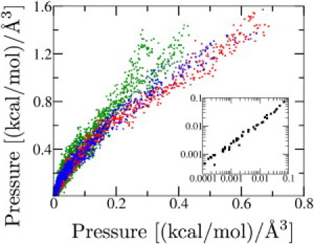
Isotropic pressure of unfolded flagellin. Radial (y axis) versus axial (x axis) pressure for nine compression simulations in cylinders of radius 5 Å (green), 7 Å (red), and 9 Å (blue). Each data point represents a 10-ps snapshot of the pressures as compression progresses (from bottom left to top right). (Inset) Radial versus axial pressure for 60 equilibrium simulations; each point represents the average pressure of a single simulation. Linear least-squares fit demonstrates paxial = 0.97 pradial.
The relationship between axial and radial pressure is paxial = 2.9 pradial, which verifies that axial and radial pressure are proportional under slow compression conditions. The axial pressure is larger than the radial pressure as the compression walls must move the flagellin tens of Ångstroms through the viscous water that is getting expelled from the shrinking cylinder. The inset to Fig. 4 presents the data for the equilibrium simulations; under equilibrium conditions, axial and radial pressure are observed to be related by paxial = 0.97 pradial, which supports isotropicity and verifies Condition 1. Movie S1 in the Supporting Material demonstrates compression simulation 9A.
Test of Condition 2
The equilibrium simulations of confined flagellin allow comparison of the radial pressure of the flagellin and the degree to which it contacts the confining cylinder, representing the channel. Fig. S5, which plots surface contact density against radial pressure for the equilibrium simulations, shows that surface contact density for each independent simulation is directly proportional to radial flagellin pressure. This result verifies that increasing flagellin pressure increases contact density, which in turn increases static friction, as stipulated in Condition 2.
Test of Condition 5
Both compression and equilibrium simulations allow characterization of pressure and density for the confined unfolded flagellin. The pressure-versus-density data are shown in Fig. 5. To test Condition 5, the data presented in Fig. 5 were fitted to Eq. 12. For the compression simulations, the axial and radial pressures (in units (kcal/mol)/Å3) relate to density by and , whereas the aggregate data are described by . The inset to Fig. 5 shows, for the equilibrium simulations, flagellin pressure and density related by . Although both types of simulation agree on β ≈ 3.2, γ from the equilibrium simulations is half that of the compression simulations. The different γ-values in equilibrium and nonequilibrium compression simulations arise from the flagellin in the compression simulation having to dynamically compress through viscous water and squeeze explicit water out of the shrinking cylinder, as it becomes increasingly occupied by compressed flagellin, which adds a compression rate-dependent pressure.
Figure 5.
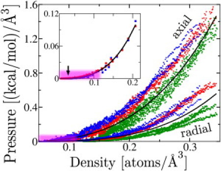
Pressure versus density of unfolded flagellin. Flagellin pressure versus density for nine compression simulations at cylinder radius 5 Å (green), 7 Å (red), and 9 Å (blue). (Upper three curves) Axial pressure. (Lower three curves) Radial pressure. Each data point represents a 10-ps snapshot as the compression progresses (from bottom left to top right). (Two black curves) Average fit of Eq. 12 to the axial (p = 36(ρ/ρ0)3) and radial (p = 26(ρ/ρ0)3.6) pressures (in units (kcal/mol)/[Angstrom symbol]3). (Inset) Radial (red) and axial (blue) pressure versus density for 60 equilibrium simulations (each data point marks the average pressure and density of a single simulation). (Black curve) Average fit of Eq. 12 to the axial and radial pressures (p = 15(ρ/ρ0)3.2). (Arrow) Location of an R = 13 Å, L = 150 Å data point used to match the Gaussian chain model to simulation data, with b (refer to Eq. 11) as the fitting parameter. (Purple highlight) Pressure and density range relevant to the flagellum.
To illustrate how far the Gaussian chain pressure-density relationship in Eq. 11 holds, we compare the prediction of this expression with the equilibrium simulation results (see data point in Fig. 5 denoted through an arrow) for the low density of ρatom = 3.07 × 10⁻² atoms/Å3 and for Natom = 2445 (i.e., = ρatom/Natom = 1.25 × 10⁻⁵ Å–3) as well as for R = 13 Å, L = 150 Å, L0 ≈ 164 × 5 Å, and T = 300 K. For a choice b = 40.5 Å, one obtains from Eq. 11 agreement with the simulated pressure p = 4.33 × 10⁻⁵ (kcal/mol)/A3. The persistence length of the flexible polymer chain would be half of the effective bond length, b (35), i.e., it would be 20 Å, which falls into the persistence length range of 5–25 Å expected for unfolded protein (45–47) ; for example, the observed and theoretical persistence length of poly-L-alanine is ∼20 Å (see (48)). Movie S1, which shows a compression simulation for R = 9 Å, is provided in the Supporting Material.
Flagellin translocation
To view the behavior of translocating flagellin in its channel environment, a 100-residue segment of flagellin was pushed through a flagellar channel as illustrated in Fig. 3. During the translocation simulation, of the many flagellin-channel interactions observed, the most striking ones are a series of salt bridges formed; a salt bridge was considered to be formed if the oxygen atom of the acidic residue and the nitrogen atom of the basic residue came within a distance of 3.2 Å. During the 52-ns simulation, 30 salt bridges were observed, 18 within flagellin and 12 between flagellin and channel. The flagellin-channel salt bridges persisted, on average, for 1–1.5 ns, corresponding to 1–1.5 Å displacement of the flagellin along the channel; at the much slower in vivo translocation rate, these salt bridges may persist much longer. Movie S2, provided in the Supporting Material, depicts the simulated translocation and highlights one such salt bridge.
The prevalence of salt bridges stimulated the investigation of the importance of charged residues across different species of flagellin. Using the VMD (38) plugin MultiSeq (49), multiple sequence alignment of both Salmonella and Escherichia coli flagellin showed a conserved SLLX motif at the C-terminus (the terminus exposed to the channel interior). In Salmonella, X is Arg494, which places a positively charged residue along the inner surface of the channel. In E. coli, X changes to GlnArg, which eliminates this positive charge; however, there is a co-mutation of Gln481 to Lys481; Lys481 is spatially adjacent to X and, thus, restores the positively charged residue to location 494. The conservation of a charged residue X suggests it to be important for translocation. Studies of the flagellum with X mutated to neutral residues could shed light on the impact of salt-bridge formation on translocation.
Agreement with experiment
It is remarkable that our simple model of flagellin translocation agrees so well with available experimental data on how friction in the channel causes the growth rate to decay exponentially with length. The strength of our model is further demonstrated by comparison with experiment.
For quantitative study of the flagellum, we first identify the physical system parameters needed in our description; Table 2 presents the required parameters. Lmax, V0, ϕ0, a, and λ are experimentally known for the flagellum, whereas β and γ are taken from the fit of Eq. 12 to the equilibrium simulations as presented in Fig. 5. The power of the flagellar pump, P (from which ftip and fstall can be directly calculated), is not experimentally known; we therefore list in Table 2 reasonable values for P and the respective values for fstall and ftip that are consistent with Eqs. 23 and 26. For quantitative analysis we will assume P = 100 (kcal/mol)/s, taken from the viral DNA packaging motor (36,37). Naturally, following our description and simulations, the system parameters listed in Table 2 can be determined for flagella of other species.
Table 2.
Flagellin translocation parameters
| Parameter | Value | Source |
|---|---|---|
| (1) Lmax | 20 μm | Iino (16) |
| (2) V0 | 91 Å/s | Iino (16) |
| (3) ϕ0 | 435 atoms/Å2/s | Iino (16) |
| (4) a | 3.7 μm | Iino (16) |
| (5) λ | 5 Å/7197 atoms | Namba et al. (15) |
| (6) R | 10 Å | Yonekura et al. (17) |
| (7) β | 3.2 | Fig. 5 |
| (8) γ | 15 (kcal/mol)/Å3 | Fig. 5 |
| (9) α |
2 × 10⁻⁴ |
Eq. 22 |
|
P |
ftip |
fstall |
| (a) 1 | 3e-6 | 8e-3 |
| (b) 10 | 9e-5 | 0.2 |
| (c) 100 | 3e-3 | 7 |
Parameters 1–6 are taken from the listed references; parameters 7 and 8 are measured from the equilibrium simulations; parameter 9 is calculated from the previously listed values and the listed equation. Regarding parameter 5, each flagellin monomer consists of 7197 atoms and contributes roughly 5 Å to flagellum length. Items a–c list three possible P values (in units (kcal/mol)/s) along with the respective ftip and fstall values (in units (kcal/mol)/Å) that are consistent with Eqs. 23 and 26.
The parameter α is neither known experimentally nor can it be determined directly for our simulations; α can, however, be computed by employing known parameters a, R, and β in Eq. 22. The very small α = 2 × 10⁻⁴, pivotal to the relationship between pressure and friction (refer to Eq. 3), suggests that very little of the radial force is translated into axial static friction, consistent with the low forces of creeping static friction. In contrast, an α-value of ∼1 would decrease the decay length from a = 3.6 μm to a = 3.6 Å, not allowing the flagellum to grow.
From Eq. 25, it can be calculated that the flagellum grows to its maximal length in roughly 24 h; this growth time is consistent with Iino (16), where it is reported that flagella grow to ∼10 μm in only a few hours, but require >10 h to reach 15 μm. We argued above (compare to Eq. 27) that the pump's stall force prevents the flagellum from infinite growth. Employing the parameters of Table 2 in Eq. 27 suggests that a stall force of 7 (kcal/mol)/Å corresponds to a maximal length of 20 μm; this stall force agrees qualitatively with the viral DNA packaging motor's stall force of ∼1 (kcal/mol)/Å (36). Fig. S4 illustrates how the force at the base of the flagellum, required to pump additional flagellin monomers into channel, grows with time; when the force at the flagellum base reaches fstall, growth ceases.
Conclusion
The exploration of flagellin translocation was facilitated by guidance of a theoretical model, which narrows the scope of properties which simulations need to address. For example, though the theoretical model describes several flagellin properties as a function of x, it also allows the properties to be expressed in terms of density independent of x; therefore, the simulations could explore friction and pressure as a function of density instead of having to simulate along an extremely long filament focusing on x dependence. The theoretical model also furnished clear tests for validation as well as a clear framework for interpreting the results in terms of actual flagellin properties.
Our model of flagellin translocation links local and short time properties to overall translocation, allowing the compression simulations, which cover only nanometers in size and nanoseconds in time, to represent the growing flagellum, which grows several micrometers in length over several hours.
The theoretical description concludes that the flagellum growth rate decreases exponentially with length because of protein compression and friction between translocating flagellin and flagellar channel increasing proportionally along the flagellum. The growth rate calculated agrees with Iino (16), who experimentally measured the growth rate decaying exponentially with length and showed it to be caused by decreasing translocation efficiency.
Acknowledgments
The authors thank Anton Arkhipov, Peter Freddolino, and Johan Strumpfer for insightful discussions.
This work was supported by the National Science Foundation (PHY0822613) and the National Institutes of Health (NIH P41-RR05969 to K.S. and Molecular Biophysics Training Grant fellowship to D.E.T.). Computer time was provided through the National Resource Allocation Committee grant (NCSA MCA93S028) from the National Science Foundation.
Supporting Material
References
- 1.Gumbart J., Schulten K. The roles of pore ring and plug in the SecY protein-conducting channel. J. Gen. Physiol. 2008;132:709–719. doi: 10.1085/jgp.200810062. [DOI] [PMC free article] [PubMed] [Google Scholar]
- 2.Neupert W., Herrmann J.M. Translocation of proteins into mitochondria. Annu. Rev. Biochem. 2007;76:723–749. doi: 10.1146/annurev.biochem.76.052705.163409. [DOI] [PubMed] [Google Scholar]
- 3.Sung W., Park P.J. Polymer translocation through a pore in a membrane. Phys. Rev. Lett. 1996;77:783–786. doi: 10.1103/PhysRevLett.77.783. [DOI] [PubMed] [Google Scholar]
- 4.Schatz G., Dobberstein B. Common principles of protein translocation across membranes. Science. 1996;271:1519–1526. doi: 10.1126/science.271.5255.1519. [DOI] [PubMed] [Google Scholar]
- 5.Lubensky D.K., Nelson D.R. Driven polymer translocation through a narrow pore. Biophys. J. 1999;77:1824–1838. doi: 10.1016/S0006-3495(99)77027-X. [DOI] [PMC free article] [PubMed] [Google Scholar]
- 6.Dubbeldam J., Milchev A., Vilgis T. Driven polymer translocation through a nanopore: A manifestation of anomalous diffusion. Europhys. Lett. 2007;79:18002. [Google Scholar]
- 7.Simon S., Peskin C., Oster G. What drives the translocation of proteins? Proc. Natl. Acad. Sci. USA. 1992;89:3770–3774. doi: 10.1073/pnas.89.9.3770. [DOI] [PMC free article] [PubMed] [Google Scholar]
- 8.Wickner W., Schekman R. Protein translocation across biological membranes. Science. 2005;310:1452–1456. doi: 10.1126/science.1113752. [DOI] [PubMed] [Google Scholar]
- 9.Muthukumar M., Kong C.Y. Simulation of polymer translocation through protein channels. Proc. Natl. Acad. Sci. USA. 2006;103:5273–5278. doi: 10.1073/pnas.0510725103. [DOI] [PMC free article] [PubMed] [Google Scholar]
- 10.Loebl H.C., Randel R., Matthai C.C. Simulation studies of polymer translocation through a channel. Phys. Rev. E. 2003;67:041913. doi: 10.1103/PhysRevE.67.041913. [DOI] [PubMed] [Google Scholar]
- 11.DePamphilis M., Alder J. Purification of Intact Flagella from Escherichia coli and Bacillus subtilis. J. Bacteriol. 1971;105:376–383. doi: 10.1128/jb.105.1.376-383.1971. [DOI] [PMC free article] [PubMed] [Google Scholar]
- 12.Blair D.F. Flagellar movement driven by proton translocation. FEBS Lett. 2003;545:86–95. doi: 10.1016/s0014-5793(03)00397-1. [DOI] [PubMed] [Google Scholar]
- 13.Yonekura K., Maki-Yonekura S., Namba K. Building the atomic model for the bacterial flagellar filament by electron cryomicroscopy and image analysis. Structure. 2005;13:407–412. doi: 10.1016/j.str.2005.02.003. [DOI] [PubMed] [Google Scholar]
- 14.Arkhipov A., Freddolino P.L., Schulten K. Coarse-grained molecular dynamics simulations of a rotating bacterial flagellum. Biophys. J. 2006;91:4589–4597. doi: 10.1529/biophysj.106.093443. [DOI] [PMC free article] [PubMed] [Google Scholar]
- 15.Namba K., Yamashita I., Vonderviszt F. Structure of the core and central channel of bacterial flagella. Nature. 1989;342:648–654. doi: 10.1038/342648a0. [DOI] [PubMed] [Google Scholar]
- 16.Iino T. Assembly of Salmonella flagellin in vitro and in vivo. J. Supramol. Struct. 1974;2:372–384. doi: 10.1002/jss.400020226. [DOI] [PubMed] [Google Scholar]
- 17.Yonekura K., Maki-Yonekura S., Namba K. Complete atomic model of the bacterial flagellar filament by electron cryomicroscopy. Nature. 2003;424:643–650. doi: 10.1038/nature01830. [DOI] [PubMed] [Google Scholar]
- 18.Mimori Y., Yamashita I., Namba K. The structure of the R-type straight flagellar filament of Salmonella at 9 Å resolution by electron cryomicroscopy. J. Mol. Biol. 1995;249:69–87. doi: 10.1006/jmbi.1995.0281. [DOI] [PubMed] [Google Scholar]
- 19.Samatey F.A., Imada K., Namba K. Structure of the bacterial flagellar protofilament and implications for a switch for supercoiling. Nature. 2001;410:331–337. doi: 10.1038/35066504. [DOI] [PubMed] [Google Scholar]
- 20.Ghosh P. Process of protein transport by the type III secretion system. Microbiol. Mol. Biol. Rev. 2004;68:771–795. doi: 10.1128/MMBR.68.4.771-795.2004. [DOI] [PMC free article] [PubMed] [Google Scholar]
- 21.Minamino T., Saijo-Hamano Y., Namba K. Domain organization and function of Salmonella FliK, a flagellar hook-length control protein. J. Mol. Biol. 2004;341:491–502. doi: 10.1016/j.jmb.2004.06.012. [DOI] [PubMed] [Google Scholar]
- 22.Hirano T., Minamino T., Macnab R. Substrate specificity classes and the recognition signal for Salmonella type III flagellar export. J. Bacteriol. 2003;185:2485–2492. doi: 10.1128/JB.185.8.2485-2492.2003. [DOI] [PMC free article] [PubMed] [Google Scholar]
- 23.Blocker A., Komoriya K., Aizawa S. Type III secretion systems and bacterial flagella: Insights into function from structural similarities. Proc. Natl. Acad. Sci. USA. 2003;100:3027–3030. doi: 10.1073/pnas.0535335100. [DOI] [PMC free article] [PubMed] [Google Scholar]
- 24.Namba K. Roles of partly unfolded conformations in macromolecular self-assembly. Genes Cells. 2001;6:1–12. doi: 10.1046/j.1365-2443.2001.00384.x. [DOI] [PubMed] [Google Scholar]
- 25.Chng C., Kitao A. Thermal unfolding simulations of bacterial flagellin: insight into its refolding before assembly. Biophys. J. 2008;94:3858–3871. doi: 10.1529/biophysj.107.123927. [DOI] [PMC free article] [PubMed] [Google Scholar]
- 26.Maki-Yonekura S., Yonekura K., Namba K. Domain movements of HAP2 in the cap-filament complex formation and growth process of the bacterial flagellum. Proc. Natl. Acad. Sci. USA. 2003;100:15528–15533. doi: 10.1073/pnas.2534343100. [DOI] [PMC free article] [PubMed] [Google Scholar]
- 27.Levy E.M. Flagellar elongation: an example of controlled growth. J. Theor. Biol. 1973;43:133–149. doi: 10.1016/s0022-5193(74)80049-4. [DOI] [PubMed] [Google Scholar]
- 28.Levy E.M. Flagellar elongation as a moving boundary problem. Bull. Math. Biol. 1974;36:265–273. doi: 10.1007/BF02461328. [DOI] [PubMed] [Google Scholar]
- 29.Mate C.M., McClelland G.M., Chiang S. Atomic-scale friction of a tungsten tip on a graphite surface. Phys. Rev. Lett. 1987;59:1942–1945. doi: 10.1103/PhysRevLett.59.1942. [DOI] [PubMed] [Google Scholar]
- 30.Fusco C., Fasolino A. Velocity dependence of atomic-scale friction: a comparative study of the one- and two-dimensional Tomlinson model. Phys. Rev. B. 2005;71:045413. [Google Scholar]
- 31.Heslot F., Baumberger T., Caroli C. Creep, stick-slip, and dry-friction dynamics: experiments and a heuristic model. Phys. Rev. E. 1994;49:4973–4988. doi: 10.1103/physreve.49.4973. [DOI] [PubMed] [Google Scholar]
- 32.Baumberger T., Gauthier L. Creeplike relaxation at the interface between rough solids under shear. J. Phys. I (Fr.) 1996;6:1021–1030. [Google Scholar]
- 33.Muser M.H. How static is static friction? Proc. Natl. Acad. Sci. USA. 2008;105:13187–13188. doi: 10.1073/pnas.0807273105. [DOI] [PMC free article] [PubMed] [Google Scholar]
- 34.Yamakawa H. Harper and Row; New York: 1971. Modern Theory of Polymer Solutions. [Google Scholar]
- 35.Kawakatsu T. Springer; Berlin, Germany: 2004. Statistical Physics of Polymers: An Introduction. [Google Scholar]
- 36.Chemla Y.R., Aathavan K., Bustamante C. Mechanism of force generation of a viral DNA packaging motor. Cell. 2005;122:683–692. doi: 10.1016/j.cell.2005.06.024. [DOI] [PubMed] [Google Scholar]
- 37.Purohit P.K., Inmdar M.M., Phillips R. Forces during bacteriophage DNA packaging and ejection. Biophys. J. 2005;88:851–866. doi: 10.1529/biophysj.104.047134. [DOI] [PMC free article] [PubMed] [Google Scholar]
- 38.Humphrey W., Dalke A., Schulten K. VMD—visual molecular dynamics. J. Mol. Graph. 1996;14:33–38. doi: 10.1016/0263-7855(96)00018-5. [DOI] [PubMed] [Google Scholar]
- 39.Phillips J.C., Braun R., Schulten K. Scalable molecular dynamics with NAMD. J. Comput. Chem. 2005;26:1781–1802. doi: 10.1002/jcc.20289. [DOI] [PMC free article] [PubMed] [Google Scholar]
- 40.MacKerell A.D., Jr., Bashford D., Karplus M. All-atom empirical potential for molecular modeling and dynamics studies of proteins. J. Phys. Chem. B. 1998;102:3586–3616. doi: 10.1021/jp973084f. [DOI] [PubMed] [Google Scholar]
- 41.Jorgensen W.L., Chandrasekhar J., Klein M.L. Comparison of simple potential functions for simulating liquid water. J. Chem. Phys. 1983;79:926–935. [Google Scholar]
- 42.Morgan D., Owen C., DeRosier D. Structure of bacterial flagellar filaments at 11 Å resolution: packing of the α-helices. J. Mol. Biol. 1995;249:88–110. doi: 10.1006/jmbi.1995.0282. [DOI] [PubMed] [Google Scholar]
- 43.Isralewitz B., Gao M., Schulten K. Steered molecular dynamics and mechanical functions of proteins. Curr. Opin. Struct. Biol. 2001;11:224–230. doi: 10.1016/s0959-440x(00)00194-9. [DOI] [PubMed] [Google Scholar]
- 44.Onufriev A., Bashford D., Case D.A. Exploring protein native states and large-scale conformational changes with a modified generalized Born model. Proteins. 2004;55:383–394. doi: 10.1002/prot.20033. [DOI] [PubMed] [Google Scholar]
- 45.Kellermayer M., Smith S., Bustamante C. Folding-unfolding transition in single titin modules characterized with laser tweezers. Science. 1997;276:1112–1116. doi: 10.1126/science.276.5315.1112. [DOI] [PubMed] [Google Scholar]
- 46.Li H., Linke W., Fernandez J.M. Reverse engineering of the giant muscle protein titin. Nature. 2002;418:998–1002. doi: 10.1038/nature00938. [DOI] [PubMed] [Google Scholar]
- 47.Lee G., Abdi K., Marszalek P.E. Nanospring behavior of ankyrin repeats. Nature. 2006;440:246–249. doi: 10.1038/nature04437. [DOI] [PubMed] [Google Scholar]
- 48.Cantor C.R., Schimmel P.R. Biophysical Chemistry. Vol. III. W. H. Freeman; New York: 1980. [Google Scholar]
- 49.Roberts E., Eargle J., Luthey-Schulten Z. MultiSeq: unifying sequence and structure data for evolutionary analysis. BMC Bioinform. 2006;7:382. doi: 10.1186/1471-2105-7-382. [DOI] [PMC free article] [PubMed] [Google Scholar]
Associated Data
This section collects any data citations, data availability statements, or supplementary materials included in this article.