Efficient spatial segmentation of large imaging mass spectrometry datasets with spatially aware clustering

Abstract

Motivation: Imaging mass spectrometry (IMS) is one of the few measurement technology s of biochemistry which, given a thin sample, is able to reveal its spatial chemical composition in the full molecular range. IMS produces a hyperspectral image, where for each pixel a high-dimensional mass spectrum is measured. Currently, the technology is mature enough and one of the major problems preventing its spreading is the under-development of computational methods for mining huge IMS datasets. This article proposes a novel approach for spatial segmentation of an IMS dataset, which is constructed considering the important issue of pixel-to-pixel variability.

Methods: We segment pixels by clustering their mass spectra. Importantly, we incorporate spatial relations between pixels into clustering, so that pixels are clustered together with their neighbors. We propose two methods. One is non-adaptive, where pixel neighborhoods are selected in the same manner for all pixels. The second one respects the structure observable in the data. For a pixel, its neighborhood is defined taking into account similarity of its spectrum to the spectra of adjacent pixels. Both methods have the linear complexity and require linear memory space (in the number of spectra).

Results: The proposed segmentation methods are evaluated on two IMS datasets: a rat brain section and a section of a neuroendocrine tumor. They discover anatomical structure, discriminate the tumor region and highlight functionally similar regions. Moreover, our methods provide segmentation maps of similar or better quality if compared to the other state-of-the-art methods, but outperform them in runtime and/or required memory.

Contact: theodore@math.uni-bremen.de

1 INTRODUCTION

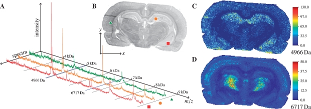
Given a thin sample (usually a tissue slice), imaging mass spectrometry (IMS) measures high-dimensional mass spectra at its spatial points, providing a hyperspectral image with a mass spectrum measured at each pixel (Fig. 1). Each mass spectrum dimension represents the abundance of molecules with this molecular mass. Currently, IMS is one of the few biochemical technologies able to establish the spatial biochemical composition of the sample in the full molecular range (small and large molecules, e.g. metabolites, lipids and proteins). Since 1970s, secondary ion mass spectrometry was the main IMS technique for surface analysis (Benninghoven and Loebach, 1971), although being unable to measure large molecules (e.g. peptides and proteins). With the advent of Matrix-assisted laser desorption ionization (MALDI) imaging mass spectrometry (Stoeckli et al., 2001), the measurement of peptides and proteins became possible what opened IMS a door to the variety of biological and biomedical problems.

Fig. 1.

An IMS dataset is a data cube. Spectra (A) are measured at spatial points of a sample (B) with spatial coordinates (x,y). Given a mass, one obtains an intensity image; examples for 4966 Da and 6717 Da are shown in (C–D).

Currently, IMS is one of the most promising innovative measurement techniques in biochemistry. IMS has proven its potential in discovery of new drugs (Solon et al., 2010; Yang et al., 2009) and cancer biomarkers (Cazares et al., 2009; Rauser et al., 2010) just to mention a few important applications. IMS was used in numerous studies leading to understanding chemical composition and biological processes, see recent reviews on this topic (Amstalden van Hove et al., 2010; Watrous et al., 2011). As for many modern biochemical techniques, in particular in proteomics (Patterson, 2003), the development of computational methods for IMS is lagging behind the technological progress. Two unsupervised problems are currently considered in IMS data processing: (i) data representation using principal component analysis (PCA) and its variants (Klerk et al., 2007), the technique standardly used for processing SIMS data, and (ii) spatial segmentation of an IMS dataset by means of spectra (or pixels) clustering (Alexandrov et al., 2010; Deininger et al., 2008; McCombie et al., 2005).

Concerning the second problem, the spatial segmentation of an IMS dataset, several approaches have been proposed. First, straightforward clustering of mass spectra, e.g. k-means (McCombie et al., 2005). Second, feature extraction with PCA and then hierarchical clustering of features (Deininger et al., 2008). Hierarchical clustering has an advantage of interactive analysis of the clustering dendrogram but needs to keep in memory the full distance matrix; several work-arounds have been proposed (Zhang et al., 1996) but none is accepted as a standard. The main drawback of using straightforward clustering of mass spectra is that it is negatively affected by the pixel-to-pixel variability issue (Alexandrov et al., 2010; Watrous et al., 2011), which is especially serious in the most popular IMS techniques, SIMS and MALDI-IMS. Underestimation of this issue leads to strong noise in the resulted segmentation maps (Alexandrov et al., 2010). As we show later, the method combining PCA with hierarchical clustering is also prone to this problem.

We have recently proposed a spatial segmentation method solving this important issue, where edge-preserving spatially-adaptive denoising (Grasmair, 2009) is applied to gray-scale images of selected masses prior to clustering (Alexandrov et al., 2010). The produced segmentation maps are significantly better than those produced without using denoising, in terms of lack of noise, discrimination of anatomical and histological details, and the number of visible regions. However, these improvements are achieved in full at a cost of using a computationally intensive edge-preserving spatially adaptive denoising method and slow high dimensional discriminant clustering. Use of a simpler methods improves the segmentation maps but not significantly due to strong and multiplicative noise in data.

In this article, we propose another original approach for spatial segmentation of IMS data with strong pixel-to-pixel variability. In general, this approach can be applied to any hyperspectral data, not necessarily IMS, but we consider segmentation of only IMS data. In (Alexandrov et al., 2010), the motivation for using the prior-to-clustering denoising was that neighbor pixels should have similar intensity at a peak mass (a mass, where not just noise is represented). Results shown by Alexandrov et al. (2010) confirm that a procedure taking into account spatial relations between pixels delivers a better quality than a straightforward pixels clustering. In this article, our approach is to take into account the spatial relations between pixels by incorporating this information directly into a clustering method. We propose two new approaches to pixels clustering, when each pixel is considered together with its neighbors. One is non-adaptive, where each pixel is clustered together with pixels from its neighborhood; neighborhoods are selected in the same manner for all pixels. The second structure-adaptive way respects the structure observable in data and, for a pixel, its neighborhood is defined taking into account similarities of spectra measured at pixels around it. In order to build efficient clustering methods based on these two ideas (non-adaptive and structure-adaptive), we use the FastMap method (Faloutsos and Lin, 1995), applying it for an efficient dimensionality reduction and, given a distance matrix, for finding points in euclidean space with similar inter-distances. Importantly, we do not keep the full distance matrix in memory using a special FastMap trick explained later in the paper.

We evaluate the proposed methods on two MALDI-IMS datasets, a rat brain coronal section without pathology (20 185 spectra) where of our interest is to recover the anatomical structure of the brain, and a section of a neuroendocrine tumor (NET) invading the small intestine (27 360 spectra) with the aim to discriminate the functionally similar regions, and, to highlight the tumor area. Both datasets have been introduced, segmented with prior-to-clustering advanced denoising, and discussed by (Alexandrov et al., 2010).

2 METHODS

2.1 Data measurement and preprocessing

Samples preparation and IMS measurements of both the rat brain and NET datasets are described in detail in Alexandrov et al. (2010). Shortly, the cryosections of 10 μm thickness were cut on a cryostat, transferred to a conductive indium-tin-oxide-coated glass slide (Bruker Daltonik GmbH, Bremen, Germany) and measured using a MALDI-TOF instrument (Autoflex III; Bruker Daltonik GmbH) using flexControl 3.0 and flexImaging 2.1 software (Bruker Daltonik GmbH). The lateral resolution was set to 80 μm. For the NET data, the Haematoxylin and Eosin (H&E) stained sections, coregistered with the MALDI-imaging results, were evaluated histologically by an experienced pathologist using a virtual slide scanner (MIRAX desk, Carl Zeiss MicroImaging GmbH, Munich, Germany).

The pre-processing was done in the ClinProTools 2.2 software (Bruker Daltonik). The spectra were baseline-corrected with the TopHat algorithm (minimal baseline width set to 10%, the default value in ClinProTools). No normalization or binning was done. Then spectra were saved into ASCII files and loaded in Matlab R2010b (The Mathworks Inc., Natick, MA, USA), where the processing was performed using our original implementation of all methods, including FastMap. The rat brain dataset comprises 20 185 spectra acquired within the slice area (120×201 pixels), each of 3045 data points covering the mass range 2.5–10 kDa; the NET dataset comprises 27 360 spectra (171×239 pixels) each of 5027 data points covering 3.2–18 kDa. For examples of intensity images for masses 4966 Da and 6717 Da for the rat brain dataset, see Figure 1; more examples are in (Alexandrov et al., 2010).

2.2 Peak picking

Selection of dataset frequent peaks: for the peak picking, we improved the approach proposed by Alexandrov et al. (2010). First, as by Alexandrov et al. (2010), for each 10th spectrum we picked its peaks with orthogonal matching pursuit (OMP) algorithm (Denis et al., 2009). This greedy algorithm searches for the specified number p_p of peaks which simultaneously are (i) high and (ii) fit at best the given peak shape (the Gaussian shape is used). OMP is not just selection of the p_p peaks most correlated with the Gaussian function. In comparison with this naive greedy approach, OMP has better theoretical properties of reconstruction peaks hidden in the noise; for more details, see (Denis et al., 2009). The peak picking for each 10th spectrum assigns to each mz-value a number of spectra in which this mz-value was selected as a peak. Finally, we take the most frequent peaks which were selected in more than τ_p% of considered spectra. The parameters of this peak picking approach are: (i) σ_p, the standard deviation of the Gaussian shape of a peak, (ii) n_p, the number of peaks selected per spectrum, and (iii) τ_p, the percentage of spectra a peak should be found in.

Alignment of masses corresponding to a peak: however, we realized, that because the Gaussian shape is just an approximation of a real peak shape and probably because of small mass shifts (the mass recalibration for each spectrum is not standardly performed in IMS), often several mz-values close to the center of a peak are selected. This redundancy in some not fully understood manner reduces the frequency of each mz-value. Thus, some, in fact frequent, peaks can be omitted as its mz-value has low frequency. Moreover, for a peak, this approach selects several masses with similar spatial intensity distribution what can influence the subsequent clustering. This effect seems to be stronger for large peaks, what leads to their increased impact on the clustering.

In order to prevent this redundant selection of several masses per peak, we grouped mz-values located close to each other (closer than σ_p, one fourth of the given peak shape) and, after calculating their mean value, move it uphill the dataset mean spectrum so that it gets in the local maximum of the mean spectrum. This simple improvement allows us to select peaks which, from an expert opinion, should be selected but were omitted before, thus increasing the sensitivity of the peak picking without drop of specificity. This topic, however, goes beyond the scope of this article which presents methods of segmentation applied to a reduced dataset after a peak picking. After peak picking, the images corresponding to picked masses are scaled so that their maximal value is one.

2.3 FastMap: distance-preserving projection

The FastMap algorithm (Faloutsos and Lin, 1995), given a distance matrix of size n×n and a euclidean space of dimension q, finds n points in this space with inter-distances close to those given in the matrix. It resembles multidimensional scaling (Hastie et al., 2009) but is more efficient having the linear in n complexity of O(nq). Moreover, although it is not well-known, for finding projections of n points, FastMap needs to calculate only n(2q+1) pairwise distances. Computing them on-the-fly, one significantly reduces the required memory. This trick is not described in the original paper (Faloutsos and Lin, 1995) but implemented by Faloutsos and Lin in their C package. We also use the FastMap algorithm as an efficient dimensionality reduction.

2.4 Spatially aware clustering

Probably, the most apparent way to embed the spatial relations between pixels into a clustering algorithm is to use a distance-based clustering where the distance d(s₁,s₂) between two spectra s₁ and s₂ measured at pixels with coordinates (x₁,y₁) and (x₂,y₂) depends on pixels from the neighborhoods of (x₁,y₁) and (x₂,y₂), for example,

(1)

where r defines the radius of the pixel neighborhood and {α_ij} are weights of spectra corresponding to pixels from the neighborhoods. It is natural to choose the weights {α_ij} which decrease with increasing i²+j² (small weights for pixels distant from the neighborhood center). For a neighborhood of radius r, we define the Gaussian weights as follows

(2)

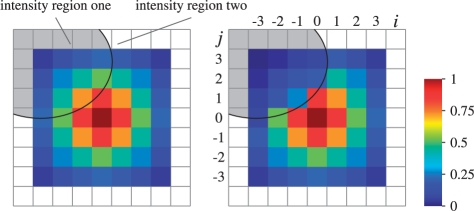
where σ is selected according to the two-sigma rule (Fig. 3A).

Fig. 3.

Left panel: Gaussian weights α_ij for a pixel neighborhood of radius r=3. Right panel: structure-adaptive weights taking into account the similarity of its spectrum to the spectra of adjacent pixels—the weights drop down when facing an intensity edge.

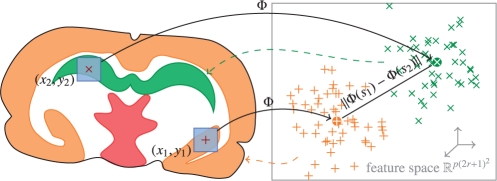
Unfortunately, this approach is memory-consuming, since it requires calculating and keeping in memory a distance matrix of size (n²−n)/2. For the NET dataset (n=27 360) this needs 1.4 GB of memory, for n=50 000 (authors processed such a dataset) 4.7 GB, for n=10⁵ (there are no restrictions to measure such a dataset with existing instruments) 18 GB. The key idea of our spatially aware clustering is inspired by the kernel methods framework. We propose to map our spectra (of length p) into a euclidean feature space ℱ using a mapping Φ, where the standard euclidean distance is

(3)

For a spectrum s∈ℝ^p, this is achieved with using

(4)

which describes the concatenation of spectra of pixels neighbor to the pixel of s, each multiplied with a square root of the corresponding weight. Naturally, the feature space ℱ is ℝ^p(2r+1)2 for such Φ; see Figure 2 for an illustration. If, as usual in IMS, n≫p (number of pixels is much more than the number of selected peaks), and r is small, then storing the mapped data of size n×p(2r+1)² is significantly cheaper than n(n−1)/2 pairwise distances.

Fig. 2.

Transformation of spectra s₁ and s₂ into feature space by taking neighborhoods around (x₁,y₁) and (x₂,y₂) into account; the mapped positions (x₁,y₁) and (x₂,y₂) are clustered in feature space.

As a last step, supposing redundancy in the mapped data, we apply the FastMap algorithm for dimensionality reduction, projecting the mapped spectra into a euclidean space of lower dimension q. Finally, clustering with an efficient vectorial clustering algorithm is performed. We propose using the k-means clustering algorithm.

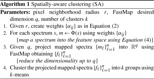
2.5 Spatially aware structure-adaptive clustering

Applying the spatially-aware clustering proposed in the previous section to IMS data, we realized that it improves the segmentation maps as compared to the straightforward clustering. However, it can smooth the edges between the anatomical or histological regions or eliminates small details; more on this in Section 3. Use of a smaller pixel neighborhood radius r solves this problem only partially, since for a smaller r the noise in the resulted segmentation map is stronger.

So, we propose another method, where for a pixel, the weights of pixels in its neighborhood are not simply Gaussian but calculated adaptively, taking into account similarities of the pixels. The key idea is as follows. For each pixel in the neighborhood, we consider the distance between its spectrum and the spectrum in the center of the neighborhood. The larger is the distance (the less similar the spectra are), the smaller is the weight. This idea is adapted from the bilateral filtering (Tomasi and Manduchi, 1998), an edge-preserving color image denoising method, where the adaptively calculated weights are used afterwards for averaging.

First, for a pixel with coordinates (x,y), we introduce

(5)

in line with Tomasi and Manduchi (1998), where λ is a parameter and δ_ij(x,y)=‖s(x+i,y+j)−s(x,y)‖₂. Then the distance between two spectra at coordinates (x₁,y₁) and (x₂,y₂) is as follows

(6)

(7)

which differs from (1) by using the adaptive weights instead of the Gaussian weights α_ij. Note that , where are reduced by multiplying with β_ij(x,y)∈(0,1]. The more similar is the spectrum s(x+i,y+j) to the spectrum s(x,y) from the neighborhood center, the larger is β_ij(x,y).

Figure 3B shows an example of the adaptive weights for a neighborhood containing spectra from two different histological regions; spectra in these regions differ significantly.

In order to eliminate the parameter λ in Equation (5) which adjusts the adaptivity of to the spectra in the neighborhood of the pixel (x,y), we propose the following approach. The value of λ(x,y) is selected for each neighborhood separately, in such a way that the largest β_ij(x,y) in this neighborhood is 1 and the smallest is exp(−2)≈0.15, what leads to

(8)

where .

Since the weights in the distance Equation (6) are determined for each pixel separately, we cannot use the concatenation like in Equation (4) to derive the transformation Φ(s(x,y)) so that . Thus, we propose to use FastMap to find projections of spectra into ℝ^q for a given q so that the pairwise distances are similar to those calculated using Equation (6). Note that we do not calculate all (n²−n)/2 pairwise distances but only n(2q+1) thanks to the FastMap trick. Finally, the points found by FastMap are clustered with k-means.

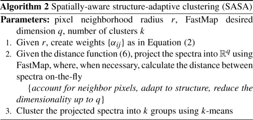
Figure 4 summarizes and illustrates the proposed segmentation methods, SA and SASA. Note that each of them has only three parameters, the pixel neighborhood radius r, the dimension q of the space where FastMap projects the mapped data to, and the number of clusters k. Later on, we will show that q is important, thus each method has only two easily interpretable parameters: r adjusts the smoothness of the segmentation map and k is simply the number of colors of the map. Both methods together with FastMap were implemented in Matlab 2010b.

Fig. 4.

Summary of the proposed spatial segmentation methods with comments.

3 RESULTS

In this section, we analyze in detail the results for the rat brain dataset. Then, we show segmentation maps for the neuroendocrine tumor dataset.

3.1 Rat brain dataset

A rat brain section is a standard example tissue in IMS. According to Watrous et al. (2011), 43% of publications on IMS of tissues consider a brain tissue. This is due to the well-known anatomical structure and clear and well-separated anatomical regions. In this section, we compare the segmentation maps produced for the rat brain slice with a schematic of the rat brain corresponding to the coronal section ~4.16 mm from Bregma drawn based on the rat brain atlas (Paxinos and Watson, 2007). The peak picking procedure with alignment of masses to peaks finds p=71 peaks.

3.1.1 Overview

Each of our proposed segmentation methods, SA (spatially adaptive, with Gaussian weights used) and SASA (spatially adaptive, with structure-adaptive weights), has only three parameters: the pixel neighborhood radius r, the dimension q of the space where FastMap projects the mapped data into, and the number of clusters k.

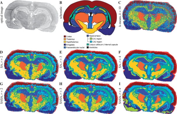
We consider segmentation maps produced for r=2, 3, 4. The FastMap dimension is q=20. The number of clusters (i.e. map colors) is k=10, what by Alexandrov et al. (2010) was found to be representative for this dataset. Figure 5 shows an optical image (A), the schematic of the anatomical structure (B), a segmentation map produced with straightforward clustering of spectra when no spatial relations between spectra are taken into account (C), and maps for SA (D–F) and SASA methods (G–I).

Fig. 5.

Rat brain dataset. (A) Optical image. (B) Schematic representation based on the rat brain atlas, reproduced from (Alexandrov et al., 2010) with permission from the American Chemical Society. (C–I) Segmentation maps, q=20, k=10. C. Straightforward k-means clustering of spectra. (D–F) SA method. (G–I) SASA method.

First, one can see that for the segmentation maps produced with both SA and SASA methods reflect the anatomical structure. Some anatomical regions (cortex, hippocampus, corpus callossum and internal capsule, amygdala) are very well represented. Note that the hippocampus has different parts (one in the middle and another close to amygdala) which still have the same color in the map (mid blue). Some regions are not well represented, e.g. a thin part of thalamus which goes around hypothalamus is not visible. However, as discussed by Alexandrov et al. (2010), this might be not a computational problem but an underrepresentation of these regions in the processed IMS dataset.

Second, our methods significantly outperform the straightforward clustering (Fig. 5C) where strong noise hides details and the whole anatomical regions. For example, in Figure 5C amygdala are not separated from hippocampus; hippocampus from the inner part of cortex and from paraventrical nuclei. Importantly, the noise in the segmentation map is a technological and computational artifact but not a property of the brain tissue; for more details on noise in MALDI-imaging, see (Alexandrov et al., 2010).

Thus, we conclude that the overall quality of the produced segmentation maps for the rat brain dataset is good. Note the blue small region interrupting the left part of cortex (Fig. 6, region A). This represents a tissue slice preparation defect (visible in the optical image as well) when the thin 10 μm tissue slice was folded during transferring it onto a glass slide.

Fig. 6.

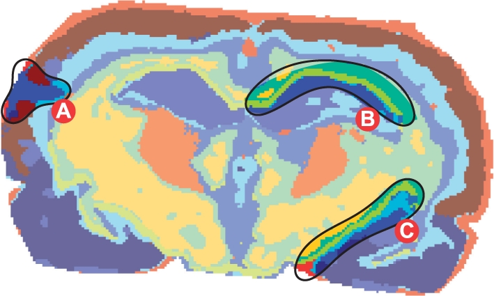
Segmentation map (SA method) for the rat brain dataset, r=3, q=20, k=10. Region A shows a tissue slice preparation defect (see in text, Section 3.1.1). Regions B and C highlight an SA-specific artifact, a layer of chartreuse yellow pixels along hippocampus (see in text, Section 3.1.4).

3.1.2 Efficiency

The efficiency of the segmentation method was the ultimate goal for us because existing advanced segmentation methods run several tens of minutes for a dataset. Tens of minutes seems acceptable because it is still less than the dataset acquisition time (several hours). However, this does not allow one to use segmentation interactively, what is of very importance in imaging applications. Moreover, at the present moment datasets with higher lateral resolution of 20 μm are becoming to be measured (Lagarrigue et al., 2010). If the rat brain slice would be measured with 20 μm resolution (instead of 80 μm used in this article), this would result into 320 000 spectra. Naturally, such a dataset would demand efficient algorithms.

Table 1 shows the runtimes for producing a segmentation map for the considered datasets not including the data loading, preprocessing and peak picking. Table 2 shows the detailed runtimes for the proposed methods. Incredibly, our methods are almost as efficient as straightforward clustering. The reasons for such efficiency are as follows: (i) the proposed approaches for incorporating spatial relations between spectra are computationally simple, (ii) the FastMap algorithm has linear complexity O(nq) in the number of spectra and requires just n(2q+1) distances calculated on-the-fly. The latter is especially important if such memory inefficient programming languages as Matlab are used for implementation.

Table 1.

Runtimes for producing a segmentation map

Dataset	(n×p)	Method	Neighborhood radius
			r=2	r=3	r=4
Rat brain	(20185×71)	SA	17 s	35 s	49 s
		SASA	19 s	32 s	49 s
		k-means*		10 s
		Denoising+HDDC*		17 min
		Denoising+kmeans*		2 min
		PCA+hierarchical*		25 s
Tumor	(27 960×62)	SA	23 s	41 s	62 s
		SASA	25 s	39 s	62 s

Runtimes on ThinkPad laptop with Intel i5 Core 2.4 GHz; data pre-processing and peak picking are not included; q=20, k=10.

*No neighborhood is exploited.

Table 2.

Detailed runtimes for SA and SASA methods

Substep	Rat brain (s)		Tumor (s)
	SA	SASA	SA	SASA
Scaling	0.01	0.01	0.01	0.01
Weights	4	4	6	6
Fastmap	25	25	32	31
k-means	5	2	3	3

ThinkPad laptop with Intel i5 Core 2.4 GHz; one iteration of k-means is used; r=3, q=20, k=10.

As for the memory space, the methods are very memory-optimized. Both methods need only n(2r+1)² memory elements for the neighbor indices, 3n distance elements in each FastMap iteration and nq memory elements for storing the FastMap projections. The SASA method stores additionally n(2r+1)² adaptive weights.

3.1.3 The role of the pixel neighborhood radius r

Figure 5D–I shows that for both SA and SASA methods, the increase of the neighborhood radius r makes the maps smoother. This is natural, because for a pixel, more pixels around it are taken into account when calculating Equations (2) or (5) what helps to reduce the pixel-to-pixel variability. On the other side, small details can be smoothed out, especially by using SA method with non-adaptive weights. For example, the central part of hippocampus in the right half loses its details visible in Figure 5D–E but not in Figure 5F, as well as the red dot in central part of the cortex (data not attributed).

3.1.4 SA method versus SASA method

Recall that the SASA method was constructed so that in a pixel neighborhood, the weights assigned to the pixels are adaptive; the more different is a spectrum from the spectrum of the central pixel, the less is the weight (Fig. 3). Thus, the ‘averaging’ in Equation (5) is done mostly among pixels similar to the central one. Comparing the maps for the SA and SASA method in Figure 5, one can see that making weights structure-adaptive prevents smoothing out the details and deteriorating of edges between different spatial regions. On the other hand, the SASA maps look noisier.

3.1.5 SA-artifacts

Comparison of the SA- and SASA-segmentation maps reveals an artifact produced by the SA method. It is a layer of chartreuse yellow pixels along hippocampus which are not visible in the SASA maps and cannot be attributed to any anatomical region. Figure 6, regions B and C, highlights the areas of the artifact. We hypothesize that this is an ‘averaging’ artifact due to weights α_ij in Equation (2) are not adaptive to the data. This is confirmed by the absence of this layer in the SA map with the smallest pixel neighborhood radius r=2 and in the SASA maps.

3.1.6 The role of the FastMap dimension q

The parameter q, the dimension of the space FastMap projects the spectra into, is the most tricky among three parameters of the SA and SASA methods. Naturally, increase of q makes the problem high-dimensional and, thus, prone to the curse of dimensionality issue. On the other hand, for any distance-preserving algorithm the quality of projection reduces with decrease of the dimension q. We propose to select q not greater than p as FastMap would project from ℝ^p into ℝ^q. For the SA method, this is motivated by the assumption that the mapping (4) into p(2r+1)²-dimensional space introduces much redundancy.

Figure 7 shows the segmentation maps for the SASA method with r=3 and k=10, for different values of the FastMap dimension q=10, 20, 50. The values of q were selected to be smaller than p=71. One can see that the maps for q=20 and 50 are very similar. The map for q=10 looks noisier with a possibly artifact region (chartreuse yellow) around the corpus callosum. Possibly, the dimension q=10 is not enough to achieve sufficient quality of the projection in contrast to q=20.

Fig. 7.

Impact of the FastMap dimension q on the segmentation map; SASA method, r=3, k=10. (A) q=10. (B) q20. (C) q=50.

3.1.7 Comparison with other methods PCA with hierarchical clustering

We have already shown that our segmentation maps excel the maps produced with straightforward clustering of spectra (Fig. 5C), mostly due to reduction of the pixel-to-pixel variability. Let us consider the method proposed by Deininger et al. (2008), where hierarchical clustering was applied to low-dimensional features extracted with PCA of spectra. Figure 8A shows the segmentation map produced with this method. As recommended in (Deininger et al., 2008), seven PCA components explaining 70% variance and the euclidean distance between extracted features were used. For the Ward linkage need much memory (for this dataset 8 GB was not enough), the complete linkage was exploited. One can see that the segmentation map is very noisy, possibly because the pixel-to-pixel variation in spectra. We have tried the average linkage as well; it produces a similarly noisy map.

Fig. 8.

Segmentation maps of other methods. (A) Hierarchical clustering (euclidean distance, complete linkage) after PCA-reduction of spectra to 70% explained variance. (B–C) With prior-to-clustering edge-preserving image denoising; k=10, moderate denoising. (B) High-dimensional discriminant clustering, reproduced from (Alexandrov et al., 2010) with permission from the American Chemical Society. (C) k-means.

3.1.8 Segmentation with prior-to-clustering edge-preserving denoising

Next, we compare our methods with advanced segmentation proposed in (Alexandrov et al., 2010), where prior-to-clustering edge-preserving denoising of mass images was used to reduce the pixel-to-pixel variability. The edge-preserving denoising due to (Grasmair, 2009) requires about 2 min for 71 images of the rat brain dataset. The segmentation map from (Alexandrov et al., 2010) for k=10 is shown in Figure 8. For clustering, High Dimensional Discriminant Clustering (HDDC) was used, the clustering method designed specially for high-dimensional data. However, its main disadvantage is the long runtimes due to using the expectation-maximization algorithm. Moreover, during an M-step it can be unstable when a cluster has a few elements or no elements, what requires starting it several times with random initializations. Although a new version of HDDC fixing these issues is planned to be included soon in the MIXMOD software (Biernacki et al., 2006), at the present time HDDC is slow. For the rat brain, one iteration takes about 50 s For k=10, at least 20 iterations are necessary because of the mentioned instability, which sums up to approximately 15 min.

For this reason, we replaced HDDC with k-means in the method proposed in (Alexandrov et al., 2010). The resulted segmentation map is shown in Figure 8. One can see that the map produced with HDDC is comparable to the maps presented in Figure 5. Moreover, as also discussed in (Alexandrov et al., 2010), k-means seems to be worse than HDDC (artifacts, less regions, detailness). The SA- and SASA-maps look better than those after k-means with prior-to-clustering denoising. The runtimes for methods considered in this section are given in Table 1, which are much longer than those for the SA and SASA methods.

3.2 The neuroendocrine tumor dataset

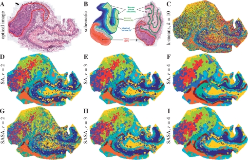
In this section, we briefly consider the segmentation maps for the second dataset, the neuroendocrine tumor invading the small intestine (ileum). This dataset differs from the rat brain dataset in the following respects: (i) it represents pathology (tumor), (ii) the tissue is more complicated, the difference between anatomical regions is not that clear, (iii) the tumor area is a heterogeneous composition of tumor cells, tumor stroma, and connective tissue. All this poses a complex challenge for a segmentation algorithm.

Figure 9 shows the optical image after H&E-staining together with 3D structure of the tissue and optical image with main functional structures as well as the segmentation maps. First, the tumor region is separated from the rest and is represented in three colors: blue, red and chartreuse yellow. This corresponds to results shown in (Alexandrov et al., 2010), although there the blue and red regions have not been separated. Moreover, the anatomical structure is represented, although the tissue flattened when put on the slide. Note the layer of brown pixels which is visible in the map after straightforward clustering (in light blue), which was not found in (Alexandrov et al., 2010).

Fig. 9.

Neuroendocrine tumor dataset. (A) Optical image after H&E staining, the tumor region is selected. (B) 3D structure of the tissue and optical image with main functional structures, reproduced from (Alexandrov et al., 2010) with permission from the American Chemical Society). (C–I) Segmentation maps, k=10. (C) Straightforward clustering of spectra. (D–E) SA method. (G–I) SASA method.

Thus, we conclude that the segmentation maps for this complex and heterogeneous tissue discriminate the tumor area, highlight the anatomical structure even after the transformation of the tissue, and excel the maps produced with the advanced prior-to-clustering denoising method by Alexandrov et al. (2010).

4 DISCUSSION

Clustering algorithm: k-means was selected as a clustering algorithm after the FastMap projection because it is a fast and reliable algorithm. Moreover, k-means optimizes the euclidean distances between the points, see e.g. Chapter 14.3.6 of (Hastie et al., 2009) (publicly available online). Thus, performing k-means in the space after FastMap projection (for both SA and SASA) is equivalent to minimize the within-point scatter between spectra where the distance between two spectra is calculated using Equations (1) or (6).

No mass-wise processing: in Alexandrov et al. (2010), denoising of each gray-scale image corresponding to a mass (channel) selected after peak picking is performed. Naturally, a channel-wise processing may be criticized as being prone to lose information presented in a combination of channels. In our methods SA and SASA, we never do channel-wise processing but consider the full spectra.

FastMap dimension q: as discussed in Section 3.1.6, the FastMap dimension q is the most tricky parameter. We have done a computational study investigating the properties of the FastMap projection and observed that increase of q changes the distances between projections, but only until some value. After this value, the distances between projections stay almost unchanged. Investigating this question can lead to a way of choosing q, and, more generally, to the way of finding the intrinsic dimension of a set of points.

Evaluation: the evaluation of produced results is an important problem, especially in an unsupervised framework, where no simple criterion (like total recognition rate) can be computed. We have tested the silhouette criterion (Rousseeuw, 1987) of separation between found clusters but have not found correspondence between the value of criterion and the visual quality of the maps. Probably, this might be explained by no clear separation between clusters.

In general, the evaluation of a spatial segmentation remains an important and unsolved problem in imaging mass spectrometry data processing, where no reference or simulated data are provided yet. Other publications on IMS segmentation, e.g. ( Alexandrov et al., 2010; Deininger et al., 2008), do not consider this question and present their methods as a data mining tool with extensive support from histologists or biologists estimating the quality of the produced segmentation maps. This is explained by the novelty of this problem and the lack of existing problems and research groups solving this problem. Certainly, in the nearest future the formal evaluation will be necessary, in particular for comparing results of different segmentation. However, any formal evaluation is a complicated task since it requires the ground truth maps for a complex enough dataset. We are working in this direction and hope to present some results soon.

In this article, which is based mostly on work by Alexandrov et al. (2010), our aim was to construct an efficient algorithm delivering segmentation maps of at least comparable quality for the datasets from Alexandrov et al. (2010) where comparison is done visually taking into account the anatomical or histological structure of the tissue sample.

Application to other hyper-spectral or multi-channel data: the proposed methods can be applied to other IMS modalities, especially those with with strong pixel-to-pixel variability (e.g. MALDI ion source, SIMS). Moreover, the SASA method can be of use for processing MALDI-IMS data obtained with the recent FT-ICR mass analyzer (Cornett et al., 2008) which produces spectra much longer than MALDI-TOF-IMS (considered in this article), of order 10⁵. Recall that the memory space and computational complexity of the SASA method does not depend on the dimensionality p of spectra but only on number of spectra n and the FastMap dimension q.

Our spatial segmentation methods can be applied for segmenting other hyper-spectral or multi-channel data, for example for terahertz imaging (Brun et al., 2010), or hyper-spectral imaging (Tarabalka et al., 2010) like that one used in German Hyperspectral Satellite Mission (Stuffler et al., 2007). The SASA method is recommended, since for this type of data usually no peak picking is performed and the dimensionality p of data is high. Moreover, in the SASA method, more appropriate distance between spectra can be selected instead of the euclidean distance in Equation (6).

3D imaging mass spectrometry: our methods can be used in spatially 3D IMS, where a spectrum is measured for a voxel with spatial coordinates (x,y,z). In this case, the number of spectra increases another order of magnitude reaching n=10⁶. For such n, pure distance-based methods which need to keep the full distance matrix in memory become inappropriate in contrast to our methods which are linear in n in memory space.

REFERENCES

- Alexandrov T., et al. Spatial segmentation of imaging mass spectrometry data with edge-preserving image denoising and clustering. J. Proteome Res. 2010;9:6535–6546. doi: 10.1021/pr100734z. [DOI] [PubMed] [Google Scholar]
- Amstalden van Hove E.R., et al. A concise review of mass spectrometry imaging. J. Chromatogr. A. 2010;1217:3946–3954. doi: 10.1016/j.chroma.2010.01.033. [DOI] [PubMed] [Google Scholar]
- Benninghoven A., Loebach E. Tandem mass spectrometer for secondary ion studies. Rev. Sci. Instr. 1971;42:49–52. [Google Scholar]
- Biernacki C., et al. Model-based cluster and discriminant analysis with the MIXMOD software. Computat. Stat. Data Anal. 2006;51:587–600. [Google Scholar]
- Brun M.-A., et al. Terahertz imaging applied to cancer diagnosis. Phys. Med. Biol. 2010;55:4615. doi: 10.1088/0031-9155/55/16/001. [DOI] [PubMed] [Google Scholar]
- Cazares L.H., et al. Imaging mass spectrometry of a specific fragment of mitogen-activated protein kinase/extracellular signal-regulated kinase kinase kinase 2 discriminates cancer from uninvolved prostate tissue. Clin. Cancer Res. 2009;15:5541–5551. doi: 10.1158/1078-0432.CCR-08-2892. [DOI] [PubMed] [Google Scholar]
- Cornett D.S., et al. MALDI-FTICR imaging mass spectrometry of drugs and metabolites in tissue. Anal. Chem. 2008;80:5648–5653. doi: 10.1021/ac800617s. [DOI] [PMC free article] [PubMed] [Google Scholar]
- Deininger S.-O., et al. MALDI imaging combined with hierarchical clustering as a new tool for the interpretation of complex human cancers. J. Proteome Res. 2008;7:5230–5236. doi: 10.1021/pr8005777. [DOI] [PubMed] [Google Scholar]
- Denis L., et al. Greedy solution of ill-posed problems: error bounds and exact inversion. Inverse Problems. 2009;25:115017. [Google Scholar]
- Faloutsos C., Lin K.-I. Proceedings of the 1995 ACM SIGMOD international conference on Management of data. San Jose, California, United States: ACM; 1995. Fastmap: a fast algorithm for indexing, data-mining and visualization of traditional and multimedia datasets; pp. 163–174. [Google Scholar]
- Grasmair M. Locally adaptive total variation regularization. In: Tai X.-C., et al., editors. Scale Space and Variational Methods in Computer Vision. Vol. 5567. Berlin/Heidelberg: Springer; 2009. pp. 331–342. Lecture Notes in Computer Science. [Google Scholar]
- Hastie T., et al. Springer Series in Statistics. New York: Springer; 2009. The Elements of Statistical Learning: Data Mining, Inference, and Prediction. [Google Scholar]
- Klerk L.A., et al. Extended data analysis strategies for high resolution imaging MS: new methods to deal with extremely large image hyperspectral datasets. Int. J. Mass Spectr. 2007;260:222–236. [Google Scholar]
- Lagarrigue M., et al. Revisiting rat spermatogenesis with MALDI imaging at 20 μm resolution. Mol. Cell. Proteomics. 2010 doi: 10.1074/mcp.M110.005991. page Epub ahead of print. [DOI] [PMC free article] [PubMed] [Google Scholar]
- McCombie G., et al. Spatial and spectral correlations in MALDI mass spectrometry images by clustering and multivariate analysis. Anal. Chem. 2005;77:6118–6124. doi: 10.1021/ac051081q. [DOI] [PubMed] [Google Scholar]
- Patterson S.D. Data analysis—the Achilles heel of proteomics. Nat. Biotech. 2003;21:221–222. doi: 10.1038/nbt0303-221. [DOI] [PubMed] [Google Scholar]
- Paxinos G., Watson C. The Rat Brain in Stereotaxic Coordinates. 6th. Amsterdam: Academic Press; 2007. [Google Scholar]
- Rauser S., et al. Classification of HER2 receptor status in breast cancer tissues by MALDI imaging mass spectrometry. J. Proteome Res. 2010;9:1854–1863. doi: 10.1021/pr901008d. [DOI] [PubMed] [Google Scholar]
- Rousseeuw P. Silhouettes: a graphical aid to the interpretation and validation of cluster analysis. J. Comput. Appl. Math. 1987;20:53–65. [Google Scholar]
- Solon E.G., et al. Autoradiography, MALDI-MS, and SIMS-MS imaging in pharmaceutical discovery and development. Am. Assoc. Pharm. Sci. J. 2010;12:11–26. doi: 10.1208/s12248-009-9158-4. [DOI] [PMC free article] [PubMed] [Google Scholar]
- Stoeckli M., et al. Imaging mass spectrometry: a new technology for the analysis of protein expression in mammalian tissues. Nat. Med. 2001;7:493–496. doi: 10.1038/86573. [DOI] [PubMed] [Google Scholar]
- Stuffler T., et al. The EnMAP hyperspectral imager—an advanced optical payload for future applications in earth observation programmes. Acta Astronaut. 2007;61:115–120. [Google Scholar]
- Tarabalka Y., et al. SVM- and MRF-based method for accurate classification of hyperspectral images. Geosci. Remote Sens. Lett., IEEE. 2010;7:736–740. [Google Scholar]
- Tomasi C., Manduchi R. ICCV '98: Proceedings of the Sixth International Conference on Computer Vision. Bombay, India: IEEE Computer Society; 1998. Bilateral filtering for gray and color images; pp. 839–846. [Google Scholar]
- Watrous J.D., et al. The evolving field of imaging mass spectrometry and its impact on future biological research. J. Mass Spectr. 2011;46:209–222. doi: 10.1002/jms.1876. [DOI] [PMC free article] [PubMed] [Google Scholar]
- Yang Y.-L., et al. Translating metabolic exchange with imaging mass spectrometry. Nat. Chem. Biol. 2009;5:885–887. doi: 10.1038/nchembio.252. [DOI] [PMC free article] [PubMed] [Google Scholar]
- Zhang T., et al. BIRCH: an efficient data clustering method for very large databases. SIGMOD Rec. 1996;25:103–114. [Google Scholar]