Abstract
Motivation: With rapidly expanding protein structure databases, efficiently retrieving structures similar to a given protein is an important problem. It involves two major issues: (i) effective protein structure representation that captures inherent relationship between fragments and facilitates efficient comparison between the structures and (ii) effective framework to address different retrieval requirements. Recently, researchers proposed vector space model of proteins using bag of fragments representation (FragBag), which corresponds to the basic information retrieval model.
Results: In this article, we propose an improved representation of protein structures using latent dirichlet allocation topic model. Another important requirement is to retrieve proteins, whether they are either close or remote homologs. In order to meet diverse objectives, we propose multi-viewpoint based framework that combines multiple representations and retrieval techniques. We compare the proposed representation and retrieval framework on the benchmark dataset developed by Kolodny and co-workers. The results indicate that the proposed techniques outperform state-of-the-art methods.
Availability: http://www.cse.iitm.ac.in/~ashishvt/research/protein-lda/.
Contact: ashishvt@cse.iitm.ac.in
1 INTRODUCTION
Following huge efforts from the structural genomics research community, protein structure databases are ever expanding. Whenever a new protein structure is determined, an important step is to identify its structural neighbors, which can provide important clues about its function and evolutionary linkages. Since the protein structure is relatively more robust than sequence during evolution, structure comparison methods can discover remote homologous proteins for a given protein. They also play a key role in understanding the diversity of structure space by analyzing the existing structure databases. In order to derive interesting scientific insights from the vast structure databases available now, highly efficient methods for comparing protein structures are required.
The success of structure comparison methods can be measured based on their effectiveness in detecting closely and remotely homologous proteins (Taylor et al., 2001). The closely homologous proteins have similar structures with relatively lesser number of insertions and deletions. On the other hand, remote homologs possess significantly different structures. The similarity in these cases can be inferred based on the similarity of structural fragments. Fragment level protein structure comparison works well in practice as demonstrated by several methods (Budowski-Tal et al., 2010; Karpen et al., 1989; Matthews et al., 1981; Zuker and Somorjai, 1989). The first fragment-based comparison method was proposed by Remington and Mathews, which performs rigid body superposition of fixed length backbone fragments from individual proteins (Matthews et al., 1981). The rigid body superposition was later used by Zuker and Somorjai to define the distance between backbone fragments while comparing them using dynamic programming (Zuker and Somorjai, 1989). The fragment-based structure comparison was also used in identification and ranking of local features (Karpen et al., 1989). For further details, the readers are referred to an excellent review paper by Taylor et al. (2001). Recently, researchers proposed an interesting vector space representation of protein structures using fragments as the bases (Budowski-Tal et al., 2010). The method, FragBag, appears to perform the task of retrieving similar structures efficiently and is the state-of-the-art method in fragment-based structure comparison.
FragBag represents each structure as a bag of fragments, which is the most basic model of retrieval proposed in text literature. The success of FragBag opens up many interesting avenues, where advanced language modeling techniques proposed in Information Retrieval (IR)/Statistical Natural Language Processing (NLP) can be adopted for representing protein structures. Such approaches are expected to achieve better performance in terms of efficiency and accuracy of identifying structural homologs. The article focuses on two important problems in this context: (i) effective protein structure representation that captures inherent relationship between fragments and facilitates efficient comparison between the structures and (ii) effective framework to address different retrieval requirements. We propose a new representation for protein structures based on latent dirichlet allocation (LDA) (Blei et al., 2003). LDA models a collection of discrete objects as a mixture of latent topics, and has been shown to work remarkably well in text and image retrieval domain. The success of LDA in text domain is attributed to effective capturing of relationship between words. Drawing a parallel, here we demonstrate that LDA indeed models relationships between fragments in protein structures effectively and achieves a competitive performance with state-of-the-art structural methods at a fraction of the computation costs. Another important contribution of this work is that we propose multi-viewpoint homology detection framework to effectively find close, as well as, remote homologous proteins for a query protein structure. This is the first attempt to adopt advanced models from IR and statistical NLP for addressing protein structure comparison problem.
2 RELATED WORK
Several methods have been proposed in literature for protein structure comparison. These methods compare a pair of protein structures, compute a quantitative measure of similarity and most often generate a structural alignment. Taylor et al. (2001) have compiled a comprehensive review describing challenges in protein structure comparison and its importance along with various proposed methods. These methods differ on the following two broad points: (i) choice of appropriate representation and (ii) algorithm for retrieval of homologous structures from the database.
The popular representation choices include (i) complete 3D coordinate information or partial coordinate information of backbone atoms, (ii) representation of various elements using their properties such as ϕ-ψ angle, solvent accessibility, etc. The first type of representation preserves sequential and topological relationships between individual elements of the structure. The methods developed to compare the first type of representation are partitioned into two: the ones using dynamic programming (DP) (Sali and Blundell, 1990; Taylor and Orengo, 1989) and others not using DP (Holm and Sander, 1996; Shindyalov and Bourne, 1998). These methods are computationally expensive and do not scale well for large number of structures. Moreover, a large number of these comparisons do not yield results since many structures are not related. To overcome these problems, researchers proposed a two stage approach widely known as the filter and match paradigm. The filtering step employs efficient and fast algorithms to obtain a small set of most likely similar proteins. These proteins are subjected to rigorous and computationally expensive structure alignment methods in the second step, which is known as a match step. The desired efficiency in filtering step is achieved by representing each protein as a vector in the space spanned by appropriate features and comparing them in the vector space. For instance, method proposed by Choi et al. (2004) and PRIDE represented protein structures using corresponding distance matrix. Rogen and Fein represented protein with topological features of backbone using knot invariants (Rogen and Fain, 2003). Zotenko and co-workers represented each protein structure as a vector of frequencies of structural models, each of which is a spatial arrangement of triplets of secondary structure elements (Zotenko et al., 2006). Several other feature-based structure representation and comparison methods have also been proposed in literature such as Friedberg et al. (2007), Tung et al. (2007), etc. For complete survey on these methods, the readers are referred to a survey by Aung and Tan (2007).
3 PROPOSED APPROACH
As mentioned in the introduction, the framework for protein structure comparison has two subproblems to be handled. In this section, we will elaborate the proposed framework to address these subproblems. These proposed techniques draw a huge motivation from statistical NLP.
3.1 Representation of proteins in topic space
The key point of the proposed approach is to represent proteins as probability distributions over latent topics. Note that the topic is an abstract concept and is represented as a multinomial distribution over fragments. Given this representation, a collection of protein structures can be modeled using three-level hierarchical Bayesian generative model known as LDA (Blei et al., 2003). Intuitively, this formalism clusters similar fragments into topics, which provides significant advantage over models that perform fragment to fragment comparison (except identity) while comparing protein structures. We explain this concept with a simple example. Suppose we are interested in comparing two documents, one containing words dog and cat and the other containing bark and mews. Naive word level comparison of the two documents reveal that they are unrelated, when they actually talk about semantically related topics (dog barking and cat mews in this case). This example can be extended to protein structures, where fragments are entities equivalent to words in the document. The fragments are grouped into a topic in a probabilistic manner and the search for homologous proteins can be performed more accurately in the topic space. Before introducing formal aspects of the problem formulation, we describe the key ingredients:
A fragment fi is the basic unit of protein structure. It is part of the fragment library of choice F. F={f1,f2,…,fL}, where L is the size of fragment library F.
A protein is a sequence of n fragments, denoted by S={fi|fiεF}. The protein structure is converted into a sequence of fragments using the method described in Budowski-Tal et al. (2010).
A universe is a collection of N proteins, denoted by U={s1,s2,…,sN}.
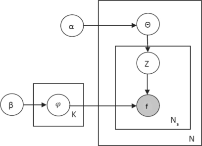
The graphical model representation of LDA is provided in Figure 1. It models the protein structure collection according to the following generative process:
Pick a multinomial distribution φz for each topic z from a dirichlet distribution with parameter β.
For each protein s, pick a multinomial distribution θs from a dirichlet distribution with parameter α.
For each fragment fi in protein structure s, pick a topic zε{1,…,K} with parameter θs.
Pick fragment fi from the multinomial distribution φz.
Fig. 1.
Graphical representation of LDA; K is the number of topics; N is the number of protein structures; Ns is the number of fragments in protein structure s.
According to the model, each protein is a mixture of latent variables z (referred to as clusters/topics), and each latent variable zi is a probability distribution over fragments. Given N proteins, K topics, L unique fragments in the collection, we can represent p(f|z) for the fragment f, with a set of K multinomial distributions φ over the L fragments, P(f|z=j)=φf(j). P(z) is modeled with a set of N multinomial distributions θ over K topics. One way to achieve is to use expectation–maximization to find the estimates of φ and θ. It suffers from local maxima issues, and its hard to model an unseen protein since it does not assume anything about θ. LDA overcomes these issues by assuming a prior distribution on θ and φ to provide a complete generative model. It uses dirichlet distribution1 for choosing priors α for θ and β for φ.
The likelihood of generating a universe of protein structure collections is
 |
Exact inference is LDA model is intractable and hence a number of approximate inference techniques such as variational methods (Blei et al., 2003), expectation propagation (Griffiths and Steyvers, 2004) and Gibbs sampling (Geman and Geman, 1984; Griffiths and Steyvers, 2004) have been proposed in the literature. We use Gibbs sampling-based inferencing to estimate φ and θ. From a sample,  and
and  are approximated using following equations after a fixed number of iterations, which is commonly known as burn in period.
| (1) |
| (2) |
Here, ni,j is the number of instances of fragment fi, assigned to topic z=j. α and β are hyperparameters that determine the smoothness of the distribution. ni,j(si) is the number of fragments in protein si that belong to topic z=j. Thus, the total number of fragments assigned to topic z=j is given by ∑v=1Vni,j(v). The total number of fragments in protein si is given by ∑t=1Tni,j(si). The terms, ∑v=1Vni,j(v) and ∑t=1Tni,j(si) are normalizing factors.
The work flow for building topic model is as follows:
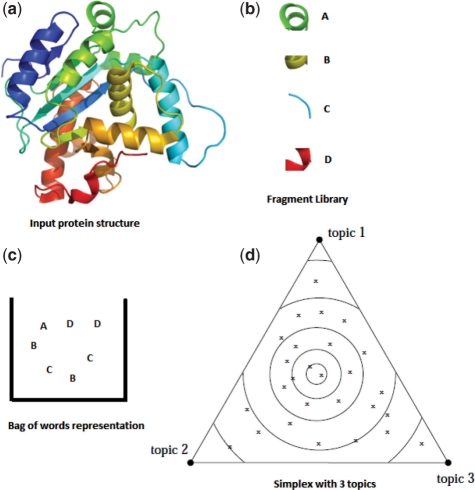
We take collection of protein structures as an input. We process each structure and obtain the corresponding fragment by matching its substructures with the library. At the end of this process, we obtain a bag of fragments for each protein. This process is depicted in Figure 2.
We learn the topic model on the collection using the machinery described earlier in this section.
Each protein is then represented as a probability distribution over the latent topics discovered by LDA.
Fig. 2.
Example protein structure with bag of fragments and topic space representations; built for a given fragment library. (a) shows an example protein structure and (b) shows a given fragment library. Each substructure in protein is compared against the fragment library and the closest matching fragment is used to represent the substructure. Thus, we obtain bag of fragments representation for protein structure as shown in (c). We model the structure as a probability distribution over latent topics. In (d) we have shown a toy representation using three topics, which forms a simplex.
3.2 Multi-viewpoint-based retrieval
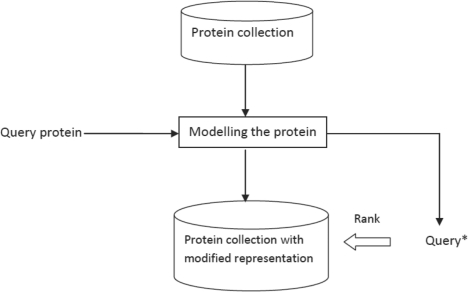
A simple framework for protein retrieval is given in Figure 3, where the universe of proteins are modeled using the representation R chosen. In order to rank the proteins based on the structural similarity for a query protein, the query protein is modeled and transformed to the same representation space R. Once the transformation is done, the protein structures in the collection are ranked based on their structural similarity with the query protein using a retrieval technique. Most simplest technique would involve a boolean vector representation for each protein. Here, the fragments from the fragment library are matched against the protein structure, and a vector of size of the fragment library is built. The vector has 1 in the position of fragments that are present and 0 in the place of fragments that are absent. And retrieval can be based on Jaccard Coefficient (Manning et al., 2008). It can be replaced by other IR techniques such as term frequency (TF), term frequency-inverse document frequency (TF-IDF), etc. The similarity metrics must be chosen according to the choice of representation (Manning et al., 2008). We refer to this family of techniques as naive vector space models.
Fig. 3.
Typical IR model.
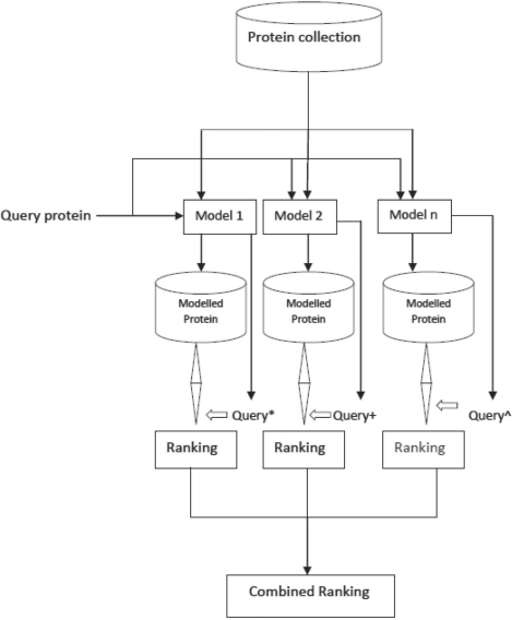
As mentioned earlier, the retrieval might have different objectives for different applications. For example, retrieving proteins that are similar, whether they are close homologs or remote homologs. Text-based IR researchers have shown that retrieval based on combination of multiple query representations, multiple representations of text documents or multiple IR techniques provide significantly improved results compared with single representation-based technique, especially when there are multiple retrieval requirements across users. These techniques are referred to as multi-viewpoint-based IR in literature (Powell and French, 1998). Schema of multi-viewpoint IR is given in Figure 4. The intuition behind doing this is: retrieval information about an author, publication or book would require exact keyword match, but querying based on topics, for example ‘sports news’, must allow more than just keyword match. Motivated by the success of multi-viewpoint-based text IR works, we propose a multi-viewpoint-based retrieval system for protein structure collection. Protein structure similarity can be captured by not only matching fragments in the protein structure, but also similar fragments (not just identity) must also be considered to help protein structure comparison. This is achieved by modeling the protein structure using LDA, which maps the fragments to a topic space using their cooccurrence information. Protein structure comparison at topic space performs a soft matching by considering similar fragments too.
Fig. 4.
Multi-viewpoint-based IR.
The proposed model combines the plain vector (boolean or frequency-based) representation of fragments in protein structure and topic space representation using LDA. Query protein and proteins in the collection are transformed into a naive vector space model and LDA representation. The retrieval techniques for both the modeling methods are different. Let us assume a simple boolean representation and a cosine similarity metric for the naive vector space model. Cosine similarity between two protein structures represented using boolean vectors A, B is given below
We refer to the similarity based on naive vector representation as FragSimilarity. LDA-based representation uses the asymmetric Kullback Leibler (KL) divergence measure to rank proteins. Asymmeric KL divergence between two proteins represented by the topic distribution vector P and Q is given below
The ranking based on these two techniques are combined using a weighted combination of similarity values. KL divergence captures the distance and not similarity value as in the case of cosine similarity. The range of values for cosine similarity (0,1) and KL divergence (−∞,0) are different. KL divergence values are normalized using min–max normalization to get normalized KL divergence measure DKLnorm, and converted into similarity value by performing 1−DKLnorm. Finally, the values are combined as follows
λ1 and λ2 denote the relative weight for the retrieval schemes based on vector representation and LDA, respectively. The model can also be extended to more representation schemes, where 0≤λi≤1 and ∑iλi=1 Comparison of various vector representations and similarity metrics are given in the Section 4.
4 EXPERIMENTAL RESULTS
The experiments are performed on FragBag dataset (Budowski-Tal et al., 2010) containing 2930 sequence non-redundant structures selected from CATH version 2.4. The dataset was constructed by using a best-of-six structural aligner using SSAP (Taylor and Orengo, 1989), STRUCTAL, DALI (Holm and Sander, 1996), LSQMAN (Kleywegt, 1996), CE (Shindyalov and Bourne, 1998) and SSM (Kolodny et al., 2005; Budowski-Tal et al., 2010). The structural neighbors of each protein are determined using threshold on structural alignment score (SAS) obtained from the alignments. The following three SAS thresholds, 2, 3.5 and 5 Å, are used to obtain close to remote homologs of the query protein. Each protein in the dataset is represented as a probability distribution over the latent topics discovered by LDA and is used as a query for evaluating performance of our method in ranking its structural neighbors. For constructing topic models, we use 7 out of 24 fragment libraries proposed by Kolodny et al. (2005) based on their performance as reported in earlier work (Budowski-Tal et al., 2010). These seven libraries are as follows: 100 (5), 300 (6), 250 (7), 600 (9), 600 (10), 400 (11) and 400 (12). Here, each library is represented with the number of constituent fragments and their size. For example, 400 (11) represents a library containing 400 fragments of size 11. The ranking performance is measured using area under the curve (AUC) of receiver operating characteristics (ROC) curve. The overall AUC value is obtained by averaging individual AUC values across 2930 query proteins. The AUC takes values between 0 and 1 and its value closer to 1 indicates higher ranking performance.
A number of similarity measures exist for comparing protein structures in topic space. We compare the performance of the following distance measures: cosine similarity (CO), Euclidean distance (EU) and KL divergence (KL) and select the one with the highest performance. The topics were discovered from proteins represented using fragments from 400 (11) library, which is chosen due to its top performance in FragBag experiments (Budowski-Tal et al., 2010). Table 1 contains the results for three different SAS thresholds: 2, 3 and 5 Å. It can be seen that KL and CO are more appropriate for SAS threshold of 2 and 5 Å, while KL performs slightly better than CO for SAS threshold of 3.5 Å. We use KL as a preferred distance measure for further analysis, since it outperforms the other two measures in most of the choices of the number of topics (Table 1).
Table 1.
Comparison of three different distance measures
| Distance | Topics |
SAS | |||||||
|---|---|---|---|---|---|---|---|---|---|
| 10 | 100 | 150 | 200 | 250 | 300 | 400 | 500 | ||
| KL | 0.85 | 0.89 | 0.9 | 0.9 | 0.9 | 0.9 | 0.9 | 0.9 | |
| EU | 0.84 | 0.87 | 0.88 | 0.88 | 0.87 | 0.87 | 0.87 | 0.87 | 2 |
| CO | 0.85 | 0.89 | 0.89 | 0.89 | 0.9 | 0.9 | 0.9 | 0.9 | |
| KL | 0.71 | 0.77 | 0.77 | 0.78 | 0.77 | 0.78 | 0.78 | 0.77 | |
| EU | 0.69 | 0.71 | 0.73 | 0.73 | 0.73 | 0.73 | 0.72 | 0.72 | 3.5 |
| CO | 0.70 | 0.73 | 0.76 | 0.76 | 0.76 | 0.77 | 0.77 | 0.77 | |
| KL | 0.68 | 0.69 | 0.69 | 0.69 | 0.68 | 0.68 | 0.68 | 0.67 | |
| EU | 0.67 | 0.67 | 0.67 | 0.66 | 0.66 | 0.65 | 0.65 | 0.65 | 5 |
| CO | 0.68 | 0.69 | 0.69 | 0.69 | 0.69 | 0.69 | 0.69 | 0.68 | |
Cosine similarity (CO), Euclidean distance (EU) and KL divergence (KL) based on average area under the curve (AUC) obtained by ranking structurally similar proteins, which are represented in topic space using 400 (11) library.
In order to select the ideal number of topics, we represented proteins with various number of topics obtained for each of the seven fragment libraries and ranking performance of our method is obtained in terms of average AUC value for each of the SAS thresholds (Table 2). The analysis reveals that the representation using 200–250 topics has the best ranking performance. We use the best performing number of topics for each library in the further analyses.
Table 2.
Selection of the best number of topics for representing proteins, using each of the seven libraries, based on their ranking performance indicated by the average AUC
| Library | Topics |
SAS | |||||||
|---|---|---|---|---|---|---|---|---|---|
| 10 | 100 | 150 | 200 | 250 | 300 | 400 | 500 | ||
| 100 (5) | 0.83 | 0.85 | 0.86 | 0.88 | 0.88 | 0.87 | 0.86 | 0.84 | |
| 300 (6) | 0.84 | 0.85 | 0.86 | 0.88 | 0.88 | 0.88 | 0.87 | 0.85 | |
| 250 (7) | 0.85 | 0.87 | 0.88 | 0.89 | 0.9 | 0.89 | 0.89 | 0.89 | |
| 600 (9) | 0.85 | 0.89 | 0.9 | 0.9 | 0.9 | 0.9 | 0.89 | 0.88 | 2 |
| 600 (10) | 0.85 | 0.88 | 0.9 | 0.9 | 0.9 | 0.9 | 0.9 | 0.88 | |
| 400 (11) | 0.85 | 0.89 | 0.9 | 0.9 | 0.9 | 0.9 | 0.9 | 0.9 | |
| 400 (12) | 0.84 | 0.89 | 0.9 | 0.9 | 0.9 | 0.89 | 0.89 | 0.87 | |
| 100 (5) | 0.70 | 0.73 | 0.73 | 0.74 | 0.73 | 0.72 | 0.72 | 0.74 | |
| 300 (6) | 0.71 | 0.74 | 0.75 | 0.76 | 0.76 | 0.76 | 0.75 | 0.75 | |
| 250 (7) | 0.71 | 0.75 | 0.75 | 0.76 | 0.76 | 0.76 | 0.76 | 0.75 | |
| 600 (9) | 0.72 | 0.77 | 0.77 | 0.78 | 0.78 | 0.78 | 0.77 | 0.77 | |
| 600 (10) | 0.72 | 0.77 | 0.77 | 0.78 | 0.78 | 0.77 | 0.77 | 0.77 | 3.5 |
| 400 (11) | 0.71 | 0.77 | 0.77 | 0.78 | 0.77 | 0.78 | 0.77 | 0.77 | |
| 400 (12) | 0.71 | 0.77 | 0.77 | 0.77 | 0.76 | 0.76 | 0.76 | 0.76 | |
| 100 (5) | 0.67 | 0.68 | 0.68 | 0.68 | 0.67 | 0.67 | 0.67 | 0.67 | |
| 300 (6) | 0.66 | 0.67 | 0.68 | 0.68 | 0.68 | 0.68 | 0.68 | 0.67 | |
| 250 (7) | 0.66 | 0.69 | 0.69 | 0.68 | 0.68 | 0.68 | 0.67 | 0.67 | |
| 600 (9) | 0.68 | 0.69 | 0.7 | 0.69 | 0.68 | 0.68 | 0.68 | 0.67 | |
| 600 (10) | 0.67 | 0.69 | 0.69 | 0.69 | 0.68 | 0.68 | 0.68 | 0.66 | 5 |
| 400 (11) | 0.68 | 0.69 | 0.69 | 0.69 | 0.68 | 0.68 | 0.68 | 0.67 | |
| 400 (12) | 0.69 | 0.7 | 0.7 | 0.7 | 0.69 | 0.69 | 0.69 | 0.67 | |
As mentioned in Section 3.2, multi-viewpoint IR combines LDA and simple vector space model with weights λ1 and λ2. In this section, we identify the best simple vector space model from the following choices: (i) term frequency (TF), (ii) term frequency and inverse document frequency (TF-IDF) and (ii) boolean (Bool). We choose cosine similarity to compare vectors, since it has been shown to work well for such representations in literature. The AUC score for different λ values are given in Table 5. The values are computed on 400(11) library, which gives the best results across different number of LDA topics (from Table 2). The analysis of Table 3 reveals that the multi-viewpoint IR with either TF or TF-IDF as a simple vector space model performs better than FragBag (Budowski-Tal et al., 2010). Overall, combining TF and LDA gives the best results (Table 3). The experiments are repeated for other libraries using the best multi-viewpoint IR model (TF and LDA) and the results for SAS thresholds 2, 3.5 and 5 are given in Tables 4, 5, 6, respectively.
Table 5.
Comparison of models built on different libraries for SAS threshold of 3.5 Å
| λ1 | 400 (12) | 600 (10) | 600 (9) | 250 (7) | 200 (6) | 100 (5) |
|---|---|---|---|---|---|---|
| 0 | 0.76 | 0.76 | 0.76 | 0.74 | 0.69 | 0.72 |
| 0.1 | 0.77 | 0.77 | 0.77 | 0.75 | 0.7 | 0.72 |
| 0.2 | 0.78 | 0.77 | 0.77 | 0.75 | 0.71 | 0.72 |
| 0.3 | 0.78 | 0.78 | 0.78 | 0.76 | 0.72 | 0.73 |
| 0.4 | 0.79 | 0.78 | 0.79 | 0.76 | 0.73 | 0.73 |
| 0.5 | 0.79 | 0.79 | 0.79 | 0.76 | 0.74 | 0.73 |
| 0.6 | 0.79 | 0.8 | 0.8 | 0.77 | 0.75 | 0.74 |
| 0.7 | 0.8 | 0.8 | 0.8 | 0.77 | 0.75 | 0.74 |
| 0.8 | 0.8 | 0.8 | 0.8 | 0.78 | 0.76 | 0.74 |
| 0.9 | 0.79 | 0.79 | 0.8 | 0.77 | 0.76 | 0.75 |
| 1 | 0.77 | 0.77 | 0.78 | 0.76 | 0.76 | 0.74 |
Here each library is denoted as X(Y), where X is the number of fragments in the library, each of length Y. The ranking performance of a given multi-viewpoint IR model for a given library is given in terms of AUC. The multi-viewpoint model contains LDA model with weight λ1 and TF vector space model with weight 1 − λ1.
Table 3.
Comparing the average AUC for various Multi-viewpoint IR methods
| λ1 | SAS=2 |
SAS=3.5 |
SAS=5 |
||||||
|---|---|---|---|---|---|---|---|---|---|
| I | II | III | I | II | III | I | II | III | |
| 0 | 0.89 | 0.87 | 0.8 | 0.77 | 0.72 | 0.64 | 0.75 | 0.73 | 0.68 |
| 0.1 | 0.89 | 0.87 | 0.81 | 0.78 | 0.73 | 0.65 | 0.75 | 0.73 | 0.69 |
| 0.2 | 0.9 | 0.88 | 0.81 | 0.78 | 0.74 | 0.66 | 0.75 | 0.73 | 0.69 |
| 0.3 | 0.9 | 0.88 | 0.82 | 0.79 | 0.75 | 0.67 | 0.75 | 0.74 | 0.7 |
| 0.4 | 0.91 | 0.89 | 0.83 | 0.79 | 0.76 | 0.69 | 0.77 | 0.74 | 0.7 |
| 0.5 | 0.91 | 0.9 | 0.85 | 0.8 | 0.77 | 0.7 | 0.75 | 0.74 | 0.71 |
| 0.6 | 0.91 | 0.9 | 0.86 | 0.8 | 0.78 | 0.72 | 0.75 | 0.73 | 0.71 |
| 0.7 | 0.91 | 0.9 | 0.88 | 0.8 | 0.78 | 0.75 | 0.75 | 0.73 | 0.71 |
| 0.8 | 0.91 | 0.91 | 0.89 | 0.8 | 0.79 | 0.77 | 0.74 | 0.72 | 0.71 |
| 0.9 | 0.91 | 0.9 | 0.9 | 0.8 | 0.78 | 0.77 | 0.72 | 0.7 | 0.7 |
| 1 | 0.9 | 0.9 | 0.9 | 0.78 | 0.78 | 0.78 | 0.68 | 0.68 | 0.68 |
The multi-viewpoint models are obtained by combining latent dirichilet allocation topic model (LDA) with weight λ1 and one of the following vector space models (i) term frequency (TF) (I), (ii) term frequency inverse document frequency (TF-IDF) (II) and (iii) boolean (BOOL) (III) with weight λ2. Since λ2=1− λ1, we have not mentioned their values explicitly in the table.
Table 4.
Comparison of models built on different libraries for SAS threshold of 2 Å
| λ1 | 400 (12) | 600 (10) | 600 (9) | 250 (7) | 200 (6) | 100 (5) |
|---|---|---|---|---|---|---|
| 0 | 0.88 | 0.88 | 0.88 | 0.87 | 0.85 | 0.86 |
| 0.1 | 0.89 | 0.89 | 0.89 | 0.88 | 0.86 | 0.86 |
| 0.2 | 0.89 | 0.89 | 0.89 | 0.88 | 0.86 | 0.86 |
| 0.3 | 0.9 | 0.9 | 0.9 | 0.88 | 0.86 | 0.86 |
| 0.4 | 0.9 | 0.9 | 0.9 | 0.89 | 0.87 | 0.86 |
| 0.5 | 0.9 | 0.91 | 0.91 | 0.89 | 0.88 | 0.87 |
| 0.6 | 0.91 | 0.91 | 0.91 | 0.89 | 0.88 | 0.87 |
| 0.7 | 0.91 | 0.91 | 0.91 | 0.9 | 0.89 | 0.87 |
| 0.8 | 0.91 | 0.91 | 0.91 | 0.9 | 0.89 | 0.87 |
| 0.9 | 0.9 | 0.91 | 0.91 | 0.9 | 0.89 | 0.87 |
| 1 | 0.89 | 0.9 | 0.9 | 0.89 | 0.88 | 0.87 |
Here each library is denoted as X(Y), where X is the number of fragments in the library, each of length Y. The ranking performance of a given multi-viewpoint IR model for a given library is given in terms of AUC. The multi-viewpoint model contains LDA model with weight λ1 and TF vector space model with weight 1−λ1.
Table 6.
Comparison of models built on different libraries for SAS threshold of 5 Å
| λ1 | 400 (12) | 600 (10) | 600 (9) | 250 (7) | 200 (6) | 100 (5) |
|---|---|---|---|---|---|---|
| 0 | 0.76 | 0.75 | 0.75 | 0.75 | 0.71 | 0.73 |
| 0.1 | 0.76 | 0.75 | 0.75 | 0.75 | 0.72 | 0.73 |
| 0.2 | 0.76 | 0.75 | 0.75 | 0.75 | 0.72 | 0.73 |
| 0.3 | 0.76 | 0.76 | 0.76 | 0.76 | 0.72 | 0.73 |
| 0.4 | 0.76 | 0.76 | 0.76 | 0.76 | 0.73 | 0.73 |
| 0.5 | 0.76 | 0.76 | 0.76 | 0.76 | 0.73 | 0.73 |
| 0.6 | 0.76 | 0.76 | 0.76 | 0.76 | 0.72 | 0.73 |
| 0.7 | 0.76 | 0.75 | 0.75 | 0.75 | 0.72 | 0.72 |
| 0.8 | 0.75 | 0.74 | 0.74 | 0.74 | 0.71 | 0.72 |
| 0.9 | 0.73 | 0.73 | 0.73 | 0.73 | 0.7 | 0.71 |
| 1 | 0.69 | 0.69 | 0.69 | 0.69 | 0.68 | 0.68 |
Here each library is denoted as X(Y), where X is the number of fragments in the library, each of length Y. The ranking performance of a given multi-viewpoint IR model for a given library is given in terms of AUC. The multi-viewpoint model contains LDA model with weight λ1 and TF vector space model with weight 1 − λ1.
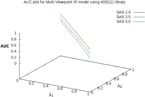
Influence of the weights λ1 and λ2 on the retrieval performance is shown in Figure 5. It can be seen that for SAS thresholds of 2 and 3.5, best performance is achieved with a higher weight for LDA representation (λ1). On the other hand, for SAS threshold of 5, best performance is achieved with a higher weight for simple vector space model (or at least equal to LDA representation). As mentioned earlier, SAS threshold 2 tends to retrieve , are for close homologs, and 5 denotes remote homologs. LDA-based representation performs better in identifying close homologs (SAS threshold of 2 Å) than the remote ones (SAS threshold of 5 Å) for a given query protein. Since the fragment functionality overlap is less as we move up the parent tree for a protein structure, exact match using naive vector space model performs better than LDA representation to identify remote homologs. Motivated by the fact that the best results are spanning different libraries, an ensemble on ranking is attempted. For a given query protein structure, similarity produced by a model, say using library 400 (11), and weights λ1=0.6, λ2=0.4 is treated as an independent hypothesis. Output of each model (combination of libraries and λ1, λ2 values) is treated as a hypothesis. The best k hypotheses (empirically chosen) are chosen and are combined using bucket of models strategy. For example, let simX(q,sd) and simY(q,sd) be the similarity scores between a query protein q and a protein sd in the database as provided by the models X and Y, respectively. Using the bucket of model strategy, the similarity between q and sd is given by sim(q,sd)=max(simX(q,sd), simY(q,sd)) This is referred to as a Combined Model. We tested it by combining three best models across SAS thresholds. The best models are 600 (9) with weights (0.8, 0.2) for SAS=2; 400 (11) with weights (0.7, 0.3) for SAS=3.5; 400 (11) with weights (0.4, 0.6) for SAS=5. Results for the Combined Model is given in Table 9.
Fig. 5.
Impact of weights, λ1 and λ2, in multi-viewpoint-based IR model. The models are constructed by combining LDA-based topic model with weight λ1 and term frequency (TF) vector space model with weight λ2.
Table 9.
AUCs of ROC curves using best-of-six gold standard
| Methods | SAS=2 | SAS=3.5 | SAS=5 | Average | Rank | Speed |
|---|---|---|---|---|---|---|
| SSM using SAS score | 0.94 | 0.9 | 0.89 | 0.91 | 1 | 13 |
| Structural using SAS score | 0.9 | 0.81 | 0.84 | 0.85 | 2 | 39 |
| Combined model | 0.92 | 0.82 | 0.75 | 0.83 | 3 | Fast |
| Structural using native score | 0.87 | 0.77 | 0.83 | 0.823 | 4 | 39 |
| Multiview model I (400,11) | 0.91 | 0.8 | 0.76 | 0.823 | 4 | Fast |
| CE using native score | 0.9 | 0.79 | 0.74 | 0.81 | 6 | 54 |
| Multiview model II (400,11) | 0.9 | 0.78 | 0.73 | 0.803 | 7 | Fast |
| FragBag Cos distance (400,11) | 0.89 | 0.77 | 0.75 | 0.803 | 7 | Fast |
| Multiview model III (400,11) | 0.89 | 0.77 | 0.7 | 0.787 | 9 | Fast |
| CE using SAS score | 0.84 | 0.72 | 0.75 | 0.77 | 10 | 54 |
| FragBag histogram intersection (600,11) | 0.87 | 0.73 | 0.7 | 0.767 | 11 | Fast |
| SGM | 0.86 | 0.71 | 0.68 | 0.75 | 12 | Fast |
| FragBag Euclidean distance (40,6) | 0.86 | 0.71 | 0.64 | 0.737 | 13 | Fast |
| Zotenko et al. (18) | 0.78 | 0.64 | 0.66 | 0.693 | 14 | Fast |
| Sequence matching by BLAST e-value | 0.76 | 0.57 | 0.5 | 0.61 | 15 | Fast |
| PRIDE | 0.72 | 0.54 | 0.51 | 0.59 | 16 | Fast |
The proposed approaches are shown in bold. Multiview model I is a combination of TF and LDA, multiview model II is a combination of TF-IDF and LDA and multiview model III is a combination of Boolean vector and LDA. The speed is given as average CPU minutes per query. If the processing time (after preprocessing of protein structure) for a query is < 0.1 s, then it is mentioned as fast.
In order to show the effectiveness of LDA-based representation over BoW representation (Budowski-Tal et al., 2010), we compare their performance on classification and clustering tasks. It can be seen that LDA representation performs better than the BoW for both the tasks, in terms of time taken and standard measures for the tasks. Table 7 has the comparison results for classification at C level classes in CATH hierarchy (4 classes). Since the dataset chosen is sparse at other levels of CATH hierarchy (has <10 members for most classes at A, T, H levels), we perform classification only at C level. Radial Basis Function network (RBF) and Naive Bayesian (NB) classifiers are used for the comparison. Results are compared in terms of root mean squared error (RMSE), ROC and accuracy. The values are obtained by averaging results across 10-fold cross validation. Table 8 contains comparative results in terms of SSE (sum of squared error) for K Means algorithm using both BoW and LDA representations.
Table 7.
Performance of BoW and LDA representations while classifying proteins at class (C) level of CATH classification
| BoW | LDA | BoW | LDA | BoW | LDA | BoW | LDA | |
|---|---|---|---|---|---|---|---|---|
| RMSE |
ROC |
Accuracy |
Time (sec) |
|||||
| RBF | 0.25 | 0.23 | 0.93 | 0.95 | 83.9 | 85.7 | 6.84 | 2.5 |
| NB | 0.33 | 0.31 | 0.9 | 0.922 | 78.6 | 80.6 | 0.58 | 0.19 |
Table 8.
Performance of BoW and LDA for protein structure clustering task
| BoW | LDA | |
|---|---|---|
| K | SSE |
|
| 4 | 8556.336 | 3371.61 |
| 10 | 8531.03 | 3417.21 |
| 20 | 8154.35 | 3348.29 |
| 50 | 7872.79 | 3093.44 |
| 100 | 7455.93 | 2880.1 |
The performance of LDA representation and retrieval based on asymmetric KL and multi-viewpoint retrieval using TF and LDA (multiview model I) are compared against naive vector space model with cosine similarity on the chosen seven libraries. For multi-viewpoint-based retrieval, the best weight combination of (λ1 and λ2) for each library is chosen for the plot. The results are shown in Figures 6, 7, 8 for SAS threshold of 2, 3.5 and 5 Å respectively. Table 9 gives overall ranking of structural and filter methods, which includes the relative positioning of proposed techniques (Kosloff and Kolodny, 2008). It is clear that our method outperforms all the filter-and-match methods. We perform a paired t-test and paired sign test with AUC values of each query obtained using proposed models and baseline state-of-the-art filter-and-match method (FragBag). Based on the statistical test, our results are significantly better than the state-of-the-art at 1% significance level. Our results are very competitive even with state-of-the-art structure comparison methods operating at the level of complete 3D representation. It must be noted that our method is much faster than these methods.
Fig. 6.
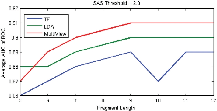
Comparison of the average AUC at SAS threshold of 2.0 Å, across libraries, obtained using TF, LDA and multiview model using the best weights from Table 3.
Fig. 7.
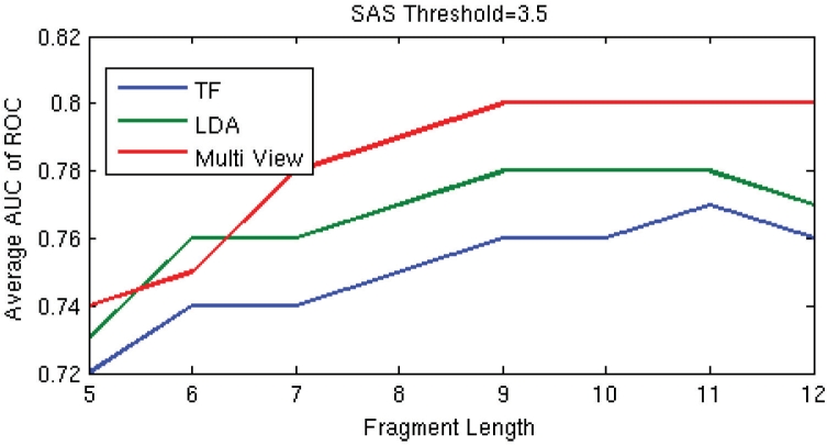
Comparison of the average AUC at SAS threshold of 3.5 Å, across libraries, obtained using TF, LDA and multiview model using the best weights from Table 4.
Fig. 8.
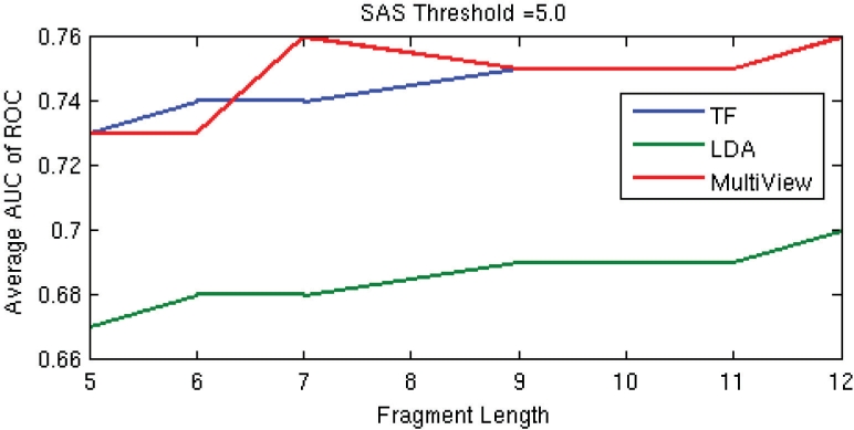
Comparison of the average AUC at SAS threshold of 5.0 Å, across libraries, obtained using TF, LDA and multiview model using the best weights from Table 5.
5 CONCLUSION
We proposed a novel framework for representation and comparison of protein structures. We demonstrated that our method outperforms most of the existing filter-and-match methods. Our results are very competitive even with the state-of-the-art structure comparison methods operating at the level of complete 3D representation. Moreover, our method is much faster than these methods. Kolodny and co-workers first proposed the use of IR techniques in protein structure comparison (Budowski-Tal et al., 2010). In this work, we have shown significant improvements by adapting more advanced models from statistical NLP literature to this task. We also take advantage of simpler models through the proposed multiview framework and built a system that can be tuned to the retrieval objectives at hand. This work has firmly established that such fragment-based models can be competitive with the structural methods. It has also opened the doors for deeper analysis, using techniques from statistical NLP, of the role that fragments play in determining the overall structure.
ACKNOWLEDGEMENTS
Dataset and tools: we thank Rachel for providing us the protein structure dataset and fragment libraries and Arun Konagurthu for fit3D code which matches a fragment with protein structure in 3D space.
Funding: Innovative Young Biotechnologist Award grant 2008 from Department of Biotechnology, Government of India (to A.V.T.).
Conflict of Interest: none declared.
Footnotes
1Dirichlet prior is a conjugate prior of multinomial distribution.
REFERENCES
- Aung Z., Tan K.-L. Rapid retrieval of protein structures from databases. Drug Discov. Today. 2007;12:732–739. doi: 10.1016/j.drudis.2007.07.014. [DOI] [PubMed] [Google Scholar]
- Blei D.M., et al. Latent dirichlet allocation. J. Mach. Learn. Res. 2003;3:993–1022. [Google Scholar]
- Budowski-Tal I., et al. FragBag, an accurate representation of protein structure, retrieves structural neighbors from the entire PDB quickly and accurately. Proc. Natl Acad. Sci. USA. 2010;107:3481–3486. doi: 10.1073/pnas.0914097107. [DOI] [PMC free article] [PubMed] [Google Scholar]
- Choi I.-G., et al. Local feature frequency profile: a method to measure structural similarity in proteins. Proc. Natl Acad. Sci. USA. 2004;101:3797–3802. doi: 10.1073/pnas.0308656100. [DOI] [PMC free article] [PubMed] [Google Scholar]
- Friedberg I., et al. Using an alignment of fragment strings for comparing protein structures. Bioinformatics. 2007;23:e219–e224. doi: 10.1093/bioinformatics/btl310. [DOI] [PubMed] [Google Scholar]
- Geman S., Geman D. Stochastic relaxation, Gibbs distributions and the Bayesian restoration of images. IEEE Trans. Pattern Anal. Mach. Intell. 1984;6:721–741. doi: 10.1109/tpami.1984.4767596. [DOI] [PubMed] [Google Scholar]
- Griffiths T.L., Steyvers M. Finding scientific topics. Vol. 101. Proc. Natl Acad. Sci. USA; 2004. pp. 5228–5235. Suppl. 1. [DOI] [PMC free article] [PubMed] [Google Scholar]
- Holm L., Sander C. Mapping the protein universe. Science. 1996;273:595–603. doi: 10.1126/science.273.5275.595. [DOI] [PubMed] [Google Scholar]
- Karpen M.E., et al. Comparing short protein substructures by a method based on backbone torsion angles. Proteins. 1989;6:155–167. doi: 10.1002/prot.340060206. [DOI] [PubMed] [Google Scholar]
- Kleywegt G.J. Use of non-crystallographic symmetry in protein structure refinement. Acta Crystallogr., Sect. D: Biol. Crystallogr. 1996;52:842–857. doi: 10.1107/S0907444995016477. [DOI] [PubMed] [Google Scholar]
- Kolodny R., et al. Comprehensive evaluation of protein structure alignment methods: scoring by geometric measures. J. Mol. Biol. 2005;346:1173–1188. doi: 10.1016/j.jmb.2004.12.032. [DOI] [PMC free article] [PubMed] [Google Scholar]
- Kosloff M., Kolodny R. Sequence-similar, structure-dissimilar protein pairs in the PDB. Proteins. 2008;71:891–902. doi: 10.1002/prot.21770. [DOI] [PMC free article] [PubMed] [Google Scholar]
- Manning C.D., et al. Introduction to Information Retrieval. New York, NY, USA: Cambridge University Press; 2008. [Google Scholar]
- Matthews B.W., et al. Relation between hen egg white lysozyme and bacteriophage T4 lysozyme: evolutionary implications. J. Mol. Biol. 1981;147:545–558. doi: 10.1016/0022-2836(81)90399-5. [DOI] [PubMed] [Google Scholar]
- Powell A.L., French J.C. Technical report CS-98-15. Charlottesville, VA, USA: 1998. The potential to improve retrieval effectiveness with multiple viewpoints. [Google Scholar]
- Rogen P., Fain B. Automatic classification of protein structure by using Gauss integrals. Proc. Natl Acad. Sci. USA. 2003;100:119–124. doi: 10.1073/pnas.2636460100. [DOI] [PMC free article] [PubMed] [Google Scholar]
- Sali A., Blundell T.L. Definition of general topological equivalence in protein structures. A procedure involving comparison of properties and relationships through simulated annealing and dynamic programming. J. Mol. Biol. 1990;212:403–428. doi: 10.1016/0022-2836(90)90134-8. [DOI] [PubMed] [Google Scholar]
- Shindyalov I.N., Bourne P.E. Protein structure alignment by incremental combinatorial extension (CE) of the optimal path. Protein Eng. 1998;11:739–747. doi: 10.1093/protein/11.9.739. [DOI] [PubMed] [Google Scholar]
- Taylor W.R., Orengo C.A. Protein structure alignment. J. Mol. Biol. 1989;208:1–22. doi: 10.1016/0022-2836(89)90084-3. [DOI] [PubMed] [Google Scholar]
- Taylor W.R., et al. Protein structure: geometry, topology and classification. Rep. Prog. Phys. 2001;64:517–590. [Google Scholar]
- Tung C.-H., et al. Kappa-alpha plot derived structural alphabet and BLOSUM-like substitution matrix for rapid search of protein structure database. Genome Biol. 2007;8:R31–R31. doi: 10.1186/gb-2007-8-3-r31. [DOI] [PMC free article] [PubMed] [Google Scholar]
- Zotenko E., et al. Secondary structure spatial conformation footprint: a novel method for fast protein structure comparison and classification. BMC Struct. Biol. 2006;6:12–12. doi: 10.1186/1472-6807-6-12. [DOI] [PMC free article] [PubMed] [Google Scholar]
- Zuker M., Somorjai R.L. The alignment of protein structures in three-dimensions. Bull. Math. Biol. 1989;51:55–78. doi: 10.1007/BF02458836. [DOI] [PubMed] [Google Scholar]


