Detecting epistatic effects in association studies at a genomic level based on an ensemble approach

Abstract

Motivation: Most complex diseases involve multiple genes and their interactions. Although genome-wide association studies (GWAS) have shown some success for identifying genetic variants underlying complex diseases, most existing studies are based on limited single-locus approaches, which detect single nucleotide polymorphisms (SNPs) essentially based on their marginal associations with phenotypes.

Results: In this article, we propose an ensemble approach based on boosting to study gene–gene interactions. We extend the basic AdaBoost algorithm by incorporating an intuitive importance score based on Gini impurity to select candidate SNPs. Permutation tests are used to control the statistical significance. We have performed extensive simulation studies using three interaction models to evaluate the efficacy of our approach at realistic GWAS sizes, and have compared it with existing epistatic detection algorithms. Our results indicate that our approach is valid, efficient for GWAS and on disease models with epistasis has more power than existing programs.

Contact: jingli@case.edu

1 INTRODUCTION

Most common diseases such as neurodegenerative diseases [e.g. Alzheimer's disease (AD) and Parkinson's disease], cardiovascular diseases, various cancers, diabetes and osteoporoses are complex diseases that involve multiple genes, their interactions, environmental factors and gene-by-environment interactions. The complex genetic architecture of complex diseases makes the task of correlating variations in DNA sequences with phenotypic differences being one of the grand challenges in biomedical research. With recent advances in genotyping technologies for assaying single nucleotide polymorphisms (SNPs), large-scale genome-wide association studies (GWAS) for complex diseases are increasingly common (e.g. Wellcome Trust Case Control Consortium, 2007). Most existing methods for GWAS are single-locus-based approaches, which examine one SNP at a time (McCarthy et al., 2008). Single-locus-based methods usually are unable to recover all involved loci, especially when individual loci have little or no marginal effects.

Detecting epistasis from GWAS is fundamentally difficult because of the large number of SNPs and relatively small number of samples. Existing SNP chips may contain up to one million SNPs and chips with a few millions of SNPs are on the pipeline. On the other hand, most studies only consist of less than a few thousands of samples per each disease. Computationally, researchers have to face the problem of the Curse of Dimensionality, whereas the search space of the problem grows exponentially with the number of involved SNPs. Statistically, one has to deal with the ‘small n big p’ problem, where the number of samples (n) is much smaller than the number of variables/SNPs (p). In general, one can view the problem as a model selection or feature selection problem with interrelated variables. However, traditional model selection approaches, most of which have to model interactions explicitly, usually are not able to incorporate so many variables in their analyses. Feature selection/reduction techniques usually are not effective in this case because of the overfitting problem as well as the problem of lack of interpretation while transforming features. Nevertheless, many approaches have been proposed over the years, though many of which are not necessarily in the context of GWAS (see Hoh and Ott, 2003 for a review).

Generally speaking, existing approaches for searching gene–gene or SNP–SNP interactions can be grouped into four broad categories. Methods in the first category rely on exhaustive search. Classical statistics such as the Pearson's χ² test or the logistic regression that are commonly used as single-locus tests for GWAS can potentially be used in searching for pairwise interactions. For example, Marchini et al. (2005) have shown that explicitly modeling of interactions between loci for GWAS with hundreds of thousands of markers is computationally feasible. They also showed that these simple methods explicitly considering interactions can actually achieve reasonably high power with realistic sample sizes under different interaction models with some marginal effects, even after adjustments of multiple testing using the Bonferroni correction. However, directly modeling of interactions is still computationally demanding and it can hardly be extended to include more than two loci. Another popular approach based on exhaustive search called multifactor dimensionality reduction (MDR) (Moore et al., 2006), which is based on partitioning all possible genotype combinations into meaningful subspaces, has the same problem of scalability. The second category consists of methods relying on stochastic search, with BEAM (Zhang and Liu, 2007) as one representative of such algorithms. Later algorithms in this category [e.g. epiMODE (Tang et al., 2009)] largely adopted and extended BEAM. BEAM uses Markov chain Monte Carlo (MCMC) sampling to infer whether each locus is a disease locus, a jointly affecting disease locus, or a background (uncorrelated) locus. The algorithm begins by assigning each locus to each group according to a prior distribution. Using the Metropolis–Hastings algorithm, it attempts to reassign the group labels to each locus. At the end, it uses a special statistic, called the B-Statistic, to infer statistical significance from the hits sampled in MCMC. This approach avoids computing all interactions, but can still theoretically find high-order interactions. The number of MCMC rounds is the primary parameter that mediates runtime, as well as power. The suggested number of MCMC rounds is in the quadratic of the number of SNPs, which limits applicability of BEAM on large datasets.

Methods in the third category are machine learning approaches such as tree-based methods or support vector machines (SVM). For example, a popular ensemble approach, Random Forests (RFs) (Breiman, 2001), has been proposed for use in association studies (Bureau et al., 2005; Lunetta et al., 2004). RFs works by first taking M bootstrap samples to grow an ensemble of decision trees each using a different subset of features. The algorithm defines an importance score for each feature/SNP and uses the score metric to rank and select SNPs. Interactions can naturally be captured by the decision tree structure. Our proposed approach also belongs to this category. But it differs from RFs from many implementation details. For example, RF uses a subset of selected SNPs in constructing bootstrap samples. However, because the number of SNPs that affect an outcome is expected to be very small compared with the total number of SNPs, a very large number of trees in RFs will not even include the target SNPs at all. This is our primary motivation to adopt the AdaBoost algorithm (Freund and Schapire, 1997; Schapire et al., 1998). Another machine learning algorithm that has been extremely popular recently is SVMs. Thus, SVMs have also been proposed as a potential GWAS algorithm (Wei et al., 2009). However, SVMs have some inherited difficulties, for example, lacking interpretability and unable to deal with large number of SNPs directly (Wei et al., 2009). Methods in the forth category rely on conditional search. In such a case, analyses are performed in stages (Evans et al., 2006; Li, 2008). A small subset of promising loci is identified in the first stage, normally using single locus methods, and multi-locus methods are used in the later stage(s) to model interactions based on the selection in the first stage. Stepwise regression has been widely used in this case and several different strategies have been studied in the literature. Methods based on conditional search can greatly reduce the computational burden by a couple of orders of magnitude, but with the risk of missing markers with small marginal effect. One should also notice that the conditional search category is more like a strategy rather than an approach. In addition to single-locus-based methods, any approaches discussed previously, especially the machine learning ones, can be used to search for candidates in the first stage.

In this article, we propose an ensemble approach based on boosting to study gene–gene interactions. We extend the basic AdaBoost algorithm by incorporating an intuitive importance score based on Gini impurity to select candidate SNPs. Permutation tests are used to control the statistical significance. We have performed extensive simulation studies using three interaction models to evaluate the efficacy of our approach at realistic GWAS sizes, and have compared it with existing epistatic detection algorithms. Our results indicate that our approach is valid, efficient for GWAS and on disease models with epistasis has more power than existing programs.

2 METHODS

2.1 Problem statement

In this article, we primarily focus on case–control designs. In the simplest form, the problem statement can be summarized as follows. Given N individuals with binary phenotypes, Y₁,…,Y_N, and each individual i with L markers. The genotypes of individual i are denoted as X_i,1,…,X_i,L, which are categorical data (usually three-valued, with an additional option for unknown). Additional information might include marker physical positions. The algorithm seeks to determine which markers, if any, are associated with the phenotype.

2.2 Algorithm details

2.2.1 Outline of the approach

Ensemble systems operate on the principle of the wisdom of crowds (Polikar, 2006). Instead of trying to create a monolithic learner or model, ensemble systems attempt to create many heterogeneous versions of simpler learners, called weak learners. The opinions of these heterogeneous experts are then combined to formulate a complete picture of the data. We extend the basic AdaBoost algorithm by incorporating an intuitive importance score based on Gini impurity to select candidate SNPs. Based on the characteristics of SNP genotype data, we select decision trees as weaker learners. In addition, the decision tree algorithm is simple to implement and can naturally capture interactions because each subsequent split is conditional on previous splits. The variable importance score is defined based on the number of trees in the ensemble that have used this variable, weighted by their performance. Permutation tests are used to control the statistical significance. Efficient designs using C++ and Python with special attention to the memory usage of SNP genotype data have been implemented. For completeness, we will describe our algorithm in four parts. First, we will describe the decision tree algorithm and how we use them as our weak learner. Second, we will describe the AdaBoost algorithm and how we use it to create an ensemble system. Third, we will describe how to calculate the statistic for variable importance estimation. Finally, we will briefly describe permutation tests for controlling type-I error.

2.2.2 Decision tree algorithm

A very simple supervised learning algorithm, the decision tree algorithm, is chosen as the weaker learner for our ensemble system, because it is easy to implement, can naturally capture interactions and satisfies the unstable learner requirement of an ensemble system. We describe the implementation details of the basic algorithm using SNP data. Decision trees are grown (trained) in a top down manner (Fig. 1). At each node, a SNP is selected and individuals at this node are partitioned into subgroups according to their genotypes. Usually, a SNP is selected to ensure largest homogeneity in the child nodes. In our implementation, we use the gain on Gini Impurity. Intuitively, when child nodes have lower impurity from a split based on an attribute (i.e. a SNP here), each child node will have purer classification. Therefore, the genotype frequencies from the two classes (case and control) are expected to be more different. More specifically, for each node, Gini Impurity is defined in Equation (1), where p_i is the probability of class i, n_i is the number of individuals in class i and N_node is the total number of individuals. A node that minimizes the Gini impurity only contains individuals of one class.

(1)

The gain of GI in a split is calculated based on Equation (2), where, d.n represents the number of individuals at a child node d, N is the number of individuals at the parent node p, the sum ranges over all child nodes, p.GI and d.GI are the Gini impurity of nodes p and d, respectively.

(2)

Usually decision trees are built with binary splits, where individuals with one value of the feature are placed into one group, and the remainder into the other. Since genotype data is three valued, we extend this to do a ternary split. This means that one split encapsulates all of the information about a SNP, instead of only a fraction like a binary split would. Each subgroup/genotype is then handled recursively until class homogeneity is reached or some stopping criterion is met. In our implementations, we impose a 5-depth limit on our trees. Though arbitrary, our preliminary tests have shown no significant changes in performance when increasing this limit.

Fig. 1.

Decision Tree example with SNPs, individual counts of two classes and the Gini impurities. The Gini gain of the split at this SNP can be calculated as (0.5−0.1*0.32−0.3*0.5−0.6*0.44)=0.004.

The Gini impurity statistic itself does not account for missing data. In our implementation, an individual with missing genotypes at one SNP is randomly assigned to one of the child nodes. This lowers the impurity of features containing missing values and naturally biases the statistic against such attributes. Despite only using marginal effects to select SNPs, decision trees can still detect some interaction. Because of the recursive partitioning, lower nodes are effectively conditioned on the value of their parents.

2.2.3 AdaBoost algorithm

AdaBoost (Freund and Schapire, 1997; Schapire et al., 1998) is a popular algorithm among a class of supervised learners called ensemble systems, which also includes RFs and Bagging. Boosting is a general technique developed by Schapire et al. (1998) that attempts to decrease the error of a weak learning algorithm using clever resampling of the training data. AdaBoost is the most popular Boosting algorithm and we use the classical algorithm without modification. The core idea of AdaBoost is to draw bootstrap samples to increase the power of a weak learner. This is done by weighting the individuals when drawing the bootstrap sample. When a weak learner instance misclassifies an individual, the weight of that individual is increased (and increased more if the weak learner instance was otherwise accurate). Thus, hard to classify individuals are more likely to be included in future bootstrap samples. In the end, the ensemble votes for class labels weighting the weak learner instances by training set accuracy. While AdaBoost was designed to decrease training set error, some have argued that instead it primarily reduces weak learner variance. This is disputed; the modern consensus is that Boosting and many other approaches can be reformulated in terms of margin theory. The goal of this approach is to maximize the distance from the class decision boundary and the training set. This improves generalization power over other algorithms that have similar test set error. The algorithm is described in Figure 2.

Fig. 2.

The modified AdaBoost algorithm with variable importance score calculation.

2.2.4 Variable importance

AdaBoost does not naturally have a feature importance score, which probably explains why it has not been used in this context before. Intuitively, within a decision tree, a variable/SNP is important if it has been chosen as an attribute earlier in building the tree, which means that it has large number of individuals and high Gini gain (more homogenous partition in child nodes). To evaluate the importance of a variable/SNP in the whole ensemble, we also consider the number of trees that the SNP has been selected and the overall performance of those trees. Therefore, we define the score for m-th SNP as

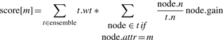(3)

where t.wt is the weight of tree t and is defined as log((1−ε_t)/ε_t), and ε_t is the training error of t. The hope is that variables that are chosen often and make good splits in effective weak learners are important. The resulting scores are arbitrarily scaled and depend on algorithm parameters such as tree pruning depth and number of AdaBoost iterations; higher is better. We use permutation tests to assess their significance.

2.2.5 Permutation tests

A permutation test is a general technique for controlling type-I error that is broadly applicable. In brief, one first creates M permutations of the class labels without replacement. For each permutation m, let T_m be the maximum test statistic in that permutation. The distribution of T_m will be used as the null distribution of the statistic. So, to determine a statistic threshold for a controlled false positive rate, say α=0.05, take the α*M-th largest value from the list of T_m. The statistical advantage of permutation tests is the tighter control for type-I error, especially for multiple testing of correlated variables. The major downside to permutation tests is that the technique greatly increases the amount of computation, which will increase linearly in the number of permutations. For simple statistics such as single-locus Pearson's χ² test, this is not terribly limiting; but for many two-locus or higher tests, it is prohibitively computationally expensive.

2.3 Implementation

We created a custom implementation of our approach using Python, scipy and C++. The primary drivers behind this decision were the performance of existing machine learning algorithm implementations such as decision trees and the need to adapt them to include the importance score calculation. If a software program is not carefully optimized, it can easily be rendered useless for GWAS. For example, representing a marker in a datatype larger than a byte can be disastrous, as memory usage could become unfeasible for standard desktop PCs. Additionally, without accessing to the internals of the decision tree and AdaBoost implementation, it would be impossible to implement our importance estimation calculation. Since there are no off-the-shelf implementations of this calculation, this point is a deal breaker. We chose the Python language due to its wide availability and ease of rapid prototyping. Thus, the first implementation of the decision trees and AdaBoost was completed very quickly and runs on multiple machines and on both the Case Western Reserve University and Ohio Supercomputer Center cluster architectures. Additionally, Python has many useful libraries, such as numpy. Numpy gives Python access to quick multidimensional arrays that we use to efficiently store the SNP data, giving Python Matlab-like functionality. Calculations on numpy arrays also run at C++ speeds, meaning the calculations are much faster than the Python equivalent. Scipy is a collection of scientific algorithms that allowed us to use off-the-shelf implementations for parts of our algorithm. Furthermore, scipy allows just-in-time compilation of C++ code to be linked with the Python interpreter.

The main performance bottlenecks are the size of the data set and the calculation for the Gini importance statistic. Numpy byte arrays solve the former problem, although a small improvement could be made with a half-byte per SNP implementation, and the later problem is solved by just-in-time compilation of C++ code. We use a heavily optimized C++ implementation of the Gini importance calculation that can operate directly upon the underlying structure of numpy arrays. We also created a GPGPU (General-purpose computing on graphics processing units) implementation using nVidia's CUDA architecture, but the performance increase was less than four-way multithreading the C++ implementation. The rest of our code is straight Python 2.4+. Despite this, the significantly more efficient C++ function for Gini importance calculation still takes >65% of our CPU time in a short profiling test. Thus, it is still the main bottleneck. This makes sense as it is a memory bound computation accessing megabytes of data; options to further optimize it are limited.

2.4 Other algorithms

2.4.1 RFs (parameters mtry, ntree)

RF were first proposed by Breiman in 2001 as an extension to Bagging (Breiman, 2001). RF, along with Bagging and Boosting, is an ensemble approach. This means that it can use many Decision Trees simultaneously to produce a superior understanding of the data. An overview of several ensemble approaches, including RFs and Boosting is available in Polikar (2006). Additionally, all of these approaches use a separate bootstrap sample for each tree. Ensemble methods are most powerful when many heterogeneous classifiers can be created, so the bootstrap samples ensure that slightly different training data are used on each tree. RFs is an improvement upon Bagging that intends to generate more varied trees. This is done by selecting mtry SNPs from the full. Each node uses a different mtry SNPs to make its decision. The parameter mtry is usually set to around the square root of the attribute set size, but different values should be tried. The number of trees in a forest is defined by the parameter ntree, which is important for performance and efficiency. Breiman's Fortran implementation of RFs has an in-built variable importance measure. First, RFs calculates the out-of-bag importance of a tree. This is calculated by using all the individuals a tree was not trained on and counting how many it correctly identifies. Then, the variable whose importance is desired is permuted, and these permuted individuals are classified by the tree. The permuted number is then subtracted from the real number, and then averaged over all the trees. This gives a raw importance score for the variable. Then, if you assume this score is independent from tree to tree, a z-score can be computed by dividing the raw score by its standard error. However, our experiments have shown that one can hardly use the significance of the derived z-score.

2.4.2 BEAM

BEAM (Zhang and Liu, 2007) is probably the seminal algorithm for epistasis analysis using stochastic search, and later algorithms in this category largely adapt it. BEAM uses MCMC sampling to attempt to infer whether each locus is a disease locus, a jointly affecting disease locus, or a background locus. This begins by assigning each locus to each group according to a prior distribution (perhaps uniform, but could include prior knowledge). Then many rounds of MCMC are run using the Metropolis–Hastings algorithm. This roughly amounts to randomly moving loci between groups. Thus, the number of MCMC rounds is the primary parameter that mediates runtime. After the MCMC, they use a special statistic, called the B-Statistic, to infer statistical significance from the hits sampled in MCMC. This approach avoids computing all interactions, but can still theoretically find high-order interactions significant.

3 RESULTS

3.1 Disease models and simulations

Assessing performance of algorithms for GWAS effectively is extremely difficult. Most algorithms deny a theoretic basis for determination of power due to the complexity of the problem. Because the true disease vectors for most complex diseases are unknown, real world data are not especially useful for assessing performance. Thus, broad, robust, blind simulation studies are an integral part of objectively assessing algorithm performance. In the current study, we will only focus on three two-locus models that have been used in previous studies (Li, 2008; Marchini et al., 2005). They were chosen primarily based on two criteria, the level of epistasis and evidences from empirical studies. Further discussion about these models and others, as well as references to some diseases that confer these theoretical models, can be found in Li and Reich (2000). The models are defined using the penetrance for each genotype combination and they are provided in Table 1 for the sake of completeness.

Table 1.

Penetrance table for two-locus additive, threshold and epistasis model

	Xj=0	Xj=1	Xj=2
Additive
Xi=0	η	η (1+θ)	η (1+2θ)
Xi=1	η (1+θ)	η (1+2θ)	η (1+3θ)
Xi=2	η (1+2θ)	η (1+3θ)	η (1+4θ)
Threshold	Xj=0	Xj=1	Xj=2
Xi=0	η	η	η
Xi=1	η	η (1+θ)	η (1+θ)
Xi=2	η	η (1+θ)	η (1+θ)
Epistasis	Xj=0	Xj=1	Xj=2
Xi=0	η	η	η (1+4θ)
Xi=1	η	η (1+2θ)	η
Xi=2	η (1+4θ)	η	η

The genotypes at the two loci (i and j) are encoded as the number of risk alleles. The penetrance of each entry is represented by a baseline η and an effect size θ.

Disease models alone are insufficient for testing GWAS algorithms. We must embed the signal into background noise somehow. There are two common approaches to this, the first being to simulate the noise simultaneously with the disease model, and the second being to embed the simulated signal into separately generated noise. While the first can more easily include complexities such as simulated linkage disequilibrium (LD) between signal SNPs and noise SNPs, the second is simpler and can have a more realistic background. We adopt the second approach in this study and use the program gs (Li and Chen, 2008) to simulate data. The program gs was developed to generate simulated data to test the performance of new algorithms on large-scale association studies. It has recently been upgraded and can provide a flexible framework to generate various interaction models. For the background noise, we use the sporadic amyotrophic lateral sclerosis (ALS) data from Schymick et al. (2007) (for historical reason) and the GWAS data from (Wellcome Trust Case Control Consortium, 2007) (denoted as WTCCC data). For each replicate, we use the gs program to create the desired two-locus interaction risk SNPs (rSNPs) and class labels. We select two random indices from the real data and replace them by the rSNPs. We then randomly selected individuals and assigned the class label and rSNPs. This ensures there is no positional or ordinal bias.

3.2 Experimental designs

Our first goal is to compare AdaBoost with RFs, both of which are machine learning algorithms and have very similar flavor. As a baseline algorithm, we also include the single- and the two-locus χ² tests in the comparison. As a note, when we performed the experience, the WTCCC data were not available to us yet. We therefore used the ALS data from Schymick et al. (2007) as the background noise. We limited our use to one chromosome with 28 818 SNPs for expediency of statistical testing and 546 individuals (we call data generated at this scale the small dataset).

Based on the performance of AdaBoost and RF, we chose AdaBoost to further compare with the program BEAM, a popular statistical approach. This time, we take a subset of the WTCCC data for background noise. For statistical expediency, we limit our noise to only the first chromosome, or 40 220 SNPs, but use a much larger sample size of 4000 individuals total (we call data generated at this scale the big dataset). While ideally, GWAS simulations should run at sizes equivalent to real studies, algorithm performance and computational resource restrictions prevent this from being possible for hundreds of replicates with thousand of permutation tests. The number of SNPs in our experiment is already two orders of magnitude above the size of simulations done in other papers (Zhang and Liu, 2007). Our results should be able to better represent algorithm performance on large datasets. We are confident that without replications, our approach can handle the real data with all SNPs without difficulty. Analysis on all the WTCCC data are still underway.

3.2.1 Model parameters and program parameters

While developing models is one step of creating an exhaustive simulation, controlling model parameters is even more important to ensure the results test the desired properties. The basic parameters in any of the three models include risk allele frequency, baseline effect (η), model effect size (θ), number of SNPs, significance level and sample size. Some derived measures include marginal effect and population prevalence. Computational resources limit the number of possible combinations. On the other hand, it is not wise to blindly choose parameter values (e.g. η). We followed the procedure below when choosing parameters for each model. First, we considered the disease to be a common one with a population prevalence of 0.1. Then, for fixed allele frequencies at both loci and a fixed effect size θ, the baseline effect η, as well as the penetrance, were obtained analytically. Coupled with the sample size, the number of markers and the overall significance level, the power of the single-locus χ² test using Bonferroni correction were numerically calculated. Details of the procedure and derivations are described elsewhere (Y.Chen and J.Li, manuscript under review). Based on the change of power, we selected different model parameters such as θ. For all the three models on the small dataset, we fixed the minor allele frequency (MAF) at 0.3 and a relative large effect size θ=2.5, which roughly corresponded to the power of 0.80 for the single-locus χ² test using Bonferroni correction on the additive model using the given number of SNPs and sample size. Given these parameters, the penetrance table for the three models was calculated and the gs program was used to generate the two disease rSNPs. For the big dataset, we additionally varied the allele frequencies and the effect sizes (θ) for each model while fixing the baseline effect η that was originally calculated based on population prevalence, to gain a whole picture on the performance of different algorithms. Therefore, different effect sizes (θ) were used for different allele frequencies and different models.

In addition to model parameters, algorithms also have their parameters. RF mainly has two parameters, the number of SNPs selected in each bootstrap sample (mtry) and the number of total decision trees in the ensemble (ntree). It is expected that the performance will be better with larger values for both parameters, with the cost of more computational burden. We first tried several different values of mtry ranging from 270 to 2700 (roughly 0.1–1% of all attributes/SNPs) and ntree ranging from 500 to 20 000 using the additive model. The power for different ratios of mtry and ntree did not seem to vary much. For example, with mtry=2700 and ntree=2000, the additive model gave a power of 45%for detecting both rSNP and 90% for detecting either; this is very similar to the results reported for mtry=270 and ntree=20 000 (49 and 90%), both of which are much better than the case using mtry=170 and ntree=2000 (16 and 62%). Based on the performance and running time, we chose mtry=270 and ntree=20 000 for RFs.

AdaBoost's main parameter is ntree, which is analogous to the ntree parameter of RFs. Since AdaBoost's trees use all of the attributes at every node, they take more time to grow but could potentially be more powerful. As such, we used ntree from 10 to 1000. Performance below 100 is pretty abysmal, and there is still a small performance gain going from 200 to 1000 (power increased from 58 to 67% to detect both SNPs for an additive model). We chose to use 200 trees for the comparison with RF on the small dataset and 1000 trees for the comparison with BEAM on the big dataset. BEAM was run with all other parameters set to their defaults, except the number of MCMC rounds was set to 16 176 484, or 1% of the number of markers squared, due to time constraints.

To obtain power, 100 replicates were generated for each parameter combination. The experimental significance level was 0.05. Permutation tests (1000 times) were used for AdaBoost and RF to control the significance level. Bonferroni correction for multiple tests was used for the single- and two-locus χ² tests on the small dataset. In such a case, they were only applied on the rSNPs. Bonferroni correction was also used for BEAM on the big dataset. On the big dataset, the single-locus χ² test was performed on the data with background noise and power using both Bonferroni correction and permutation tests was recorded.

3.3 AdaBoost versus RF

3.3.1 Power

Figure 3 shows the power to select rSNPs across the three interaction models by the four algorithms. We compare the ability to detect either locus or both loci across the algorithms. The single-locus χ² test is outperformed by every other algorithm in every test, especially in the epistatic case. Coupled with the fact that AdaBoost and RFs can still effectively be run on the large datasets produced by high-throughput SNP chips, this strongly supports their everyday use. At the same time, the reason that the power of the χ² test is low might be due to the Bonferroni correction, which was known to be conservative. We therefore also used the permutation tests for the χ² test on the large dataset. Additionally, the two-locus χ² test outperforms both of the machine learning algorithms, and is very powerful for the epistatic model. This is not surprising because all three models are two-locus models. The multiple testing penalization for the two-locus χ² test prevents it from significantly outperforming the machine learning algorithms, except when considering the epistatic model with low marginal effects. AdaBoost is slightly better than RFs for the additive model and significantly better for the epistatic model. We suspect this is due to the difference in these two algorithms. For the additive model, any splits which do not contain at least one of the rSNPs in the mtry SNPs for RFs is useless. With such large datasets and only two rSNPs, this happens reasonably often. With the epistatic model, this effect is even stronger since having the second rSNP in contention after a split on the first is the same as a conditional probability. By using all SNPs to build the trees, AdaBoost seems to have more power. However, RF performs slightly better than AdaBoost on the threshold model. This makes sense because it does not help to have the second locus around with the threshold model. Furthermore, AdaBoost could potentially have similar power if run for a similar amount of time. Indeed, when we increased the number of trees from 200 to 1000, the AdaBoost performance improves to 0.58 to detect both and 0.90 to detect either, providing better results while still running in less time than RFs. Permutation was also used for RFs, because the z-score it generated cannot be used directly. For a significance level of 0.05, usually several hundreds of variables were reported significant. We hypothesize that this is because the z-score argument for the RFs importance statistic only holds for ensembles where the raw score is independent from tree to tree. Growing large amounts of data when the attribute set is almost entirely noise could violate this property, rendering the statistic invalid.

Fig. 3.

Comparison of power to detect rSNPs across models. All models here use θ=2.5 and allele frequency of 0.3. Number of SNPs is 28 818 and number of samples is 546. χ²_B: single-locus χ² test with Bonferroni correction; AB: AdaBoost; 2-χ²_B: two-locus χ² test with Bonferroni correction; 1+: detecting at least one locus; 2: detecting both loci. Similar notations are used in Figures 4 and 5 and Tables 2 and 3.

3.3.2 Performance as two-stage selection algorithms

In addition to the normal use of AdaBoost in detecting significant SNPs, it can also be used in the first stage of a multi-stage analysis to select important candidate SNPs. Instead of determining a significant threshold using permutation tests, one can simply pick the top-k important SNPs. Depending on the algorithm to be used in Stage 2, k can be selected based on the amount of computational time available. By doing so, we can avoid the permutation test which is usually a tremendous computational burden. We therefore examined the probability to place the rSNPs into the top-k (k=50, 500) reported SNPs for both RFs and AdaBoost, regardless of their significance. The AdaBoost approach vastly outperforms RFs (Fig. 4). It never fails to report at least one, even in the k=50 case. Furthermore, the probability to detect both never drops <93%. However, the probability of RF to detecting both rSNPs is around 50%. We further examined the absolute ranks and scores of rSNPs. RFs tends to show very strong signal when it detects an rSNP, but sometimes missing them entirely. AdaBoost is much more consistent, and the rSNPs almost always fall near the top of the importance list. This again might be due to the subspace sampling of RF when constructing bootstrap samples.

Fig. 4.

The probability that either or both rSNPs were found in the top 500/50 SNPs by AdaBoost (AB) and RF for additive (A), threshold (T) and epistasis (E) model, respectively.

3.3.3 Computational resources

We ran our calculations on Ohio Supercomputing Center's Glenn Cluster, which has 2.6 GHz Dual-Core Opteron CPUs. Despite offering performance similar to or worse than the AdaBoost approach, RFs was run for much longer (90 min versus 4 min by AdaBoost for one replicate on one CPU node) and used more memory (24 MB versus 10 MB of physical memory, and 74 MB versus 42 MB virtual memory). This somewhat contradicts the fact that RFs should run faster because it only looks at mtry attributes at once. RFs V5.1 is the original implementation written in Fortran. Our version of AdaBoost was custom written using a mixture of Python and C++. While RFs is completely written in a high-performance language, our implementation could have an advantage from being targeted specifically at SNP data.

3.4 AdaBoost versus BEAM

3.4.1 Power

This section will detail results from our simulation study using the WTCCC data as background noise and signals from the same three models with different parameters. We compared four algorithms: single-locus χ² test with Bonferroni correction for multiple testing, the χ² test using permutation tests derived significance thresholds, AdaBoost with 1000 trees and finally the BEAM algorithm. These algorithms were chosen to allow us to use fundamentally different algorithms while respecting our limited computational resources.

Figure 5 shows the results on the two-locus additive model for θ=0.2, 0.35, 0.5, and risk allele frequency =0.1, 0.3 and 0.5. When the signal is low (θ = 0.2), AdaBoost has the best performance, followed by the χ² with the permutation tests. BEAM and χ² with the Bonferroni correction have the similar power. We suspect that the gain of AdaBoost was due to the recursive partitioning. An additive model does not have direct interaction between the loci's effects, but even so, the presence of multiple effect loci means that the data looks noisier to a single locus test. Recursive partitioning partially shields lower splits from this noise by condition on the split feature's values. Thus, for the additive model, the test at the second locus will get done three times (each on roughly one-third of the data), but the distribution of class labels in these nodes has been perturbed such that the cases tend to avoid the controls. This effectively removes much of the noise for the second test. When the signal is high (θ=0.35, 0.5), all methods performed similarly and have roughly the same characteristics. However, AdaBoost seems to have lower power when allele frequency is 0.1. This can be potentially explained by the use of Gini index in the importance score and in the decision tree algorithm. We discuss this phenomenon and possible improvement in the final section.

Fig. 5.

Power comparisons of the four approaches (χ²_P: χ² using permutation, χ²_B: χ² using Bonferroni correction, AB: AdaBoost and BEAM) detecting at least one (1+) or both (2) on the two-locus additive models for different effect sizes (θ) and different allele frequencies.

On the threshold model, AdaBoost outperforms all others for the MAF in the range of 0.2–0.5 (Table 2), and is the only algorithm to detect both loci in a nontrivial fraction of the replicates when the signal is low. Additionally, we can see that BEAMs power is lower than the χ² test using permutation, while roughly tracks that of Bonferroni corrected χ² test until the MAF=0.5 case. Since the threshold model has inherently lower signal at MAF=0.1, we show the result with larger θs for this case. Most of the approaches perform very similarly in this case, with AdaBoost having slightly reduced power compared with others, which is similar to the additive model.

Table 2.

Power comparisons on the two-locus threshold model, for different MAFs and effect sizes (θ)

MAF	θ	χ2_P 1+	χ2_B 1+	AB 1+	BEAM 1+	χ2_P 2	χ2_B 2	AB 2	BEAM 2
0.2	0.4	0	0	0.01	0	0	0	0	0
0.3	0.4	0.08	0.08	0.13	0.08	0	0	0	0
0.4	0.4	0.26	0.25	0.39	0.25	0.01	0.01	0.07	0.01
0.5	0.4	0.23	0.17	0.29	0.18	0	0	0.05	0
0.2	0.5	0.02	0.02	0.03	0.02	0	0	0	0
0.3	0.5	0.29	0.26	0.39	0.26	0.04	0.03	0.1	0.03
0.4	0.5	0.52	0.45	0.69	0.45	0.11	0.07	0.18	0.07
0.5	0.5	0.52	0.46	0.65	0.47	0.13	0.1	0.21	0.1
0.2	0.6	0.12	0.09	0.16	0.1	0.01	0.01	0.03	0
0.3	0.6	0.62	0.54	0.73	0.54	0.21	0.17	0.23	0.17
0.4	0.6	0.86	0.81	0.93	0.82	0.47	0.41	0.56	0.41
0.5	0.6	0.86	0.85	0.92	0.85	0.38	0.29	0.48	0.29
0.1	1.8	0.35	0.34	0.31	0.34	0.05	0.04	0.03	0.07
0.1	2.1	0.6	0.59	0.51	0.59	0.15	0.12	0.05	0.13
0.1	2.4	0.87	0.85	0.84	0.85	0.41	0.35	0.36	0.35

The four approaches are χ²_P: single-locus χ² test with Permutation correction; χ²_B: single-locus χ² test with Bonferroni correction; AB: AdaBoost; BEAM: the BEAM algorithm; 1+: detecting at least one locus; 2: detecting both loci.

The epistasis model is intended as an extreme epistasis case. Nevertheless, unless the MAF is close to 0.5, there are still non-trivial marginal effects in the model. Table 3 shows the results of the four approaches. Generally speaking, all approaches perform similarly when allele frequency is <0.3. The relative performance of AdaBoost over other approaches increased dramatically with the increase of allele frequency, in which case the marginal effect getting smaller and the interaction effect getting large. Initially, for allele frequency of 0.1 and 0.2, our approach is not as good as the other three. It outperformed the other three when the frequency is 0.3 and significantly outperformed other three when the frequency is 0.4. BEAM has slightly increased power compared with the Bonferroni corrected χ² test for detecting two loci, showing it is sometimes detecting some epistasis effect. But in most cases, the power of the two was very similar, and was slightly lower than the permutation χ² test. The allele frequency of 0.5 is a special case because it is the only disease model we examined with absolutely zero marginal effect. Therefore, interaction effects are extremely important as they are the only effective way to detect association. The difficulty of this problem is evident, as the only approach to post any results was ours with a measly 0.05 power, even with θ=1.2.

Table 3.

Power comparisons on the two-locus epistasis model, for different MAFs and effect sizes (θ)

MAF	θ	χ2_P 1+	χ2_B 1+	AB 1+	BEAM 1+	χ2_P 2	χ2_B 2	AB 2	BEAM 2
0.1	0.3	0.01	0.01	0	0	0	0	0	0
0.2	0.3	0.47	0.36	0.3	0.38	0.07	0.03	0.04	0.03
0.3	0.3	0.26	0.21	0.29	0.22	0	0	0.03	0
0.1	0.35	0.08	0.04	0	0.08	0	0	0	0
0.2	0.35	0.65	0.64	0.56	0.65	0.2	0.18	0.14	0.19
0.3	0.35	0.47	0.4	0.54	0.4	0.07	0.06	0.18	0.09
0.1	0.4	0.15	0.12	0.01	0	0.01	0	0	0
0.2	0.4	0.89	0.86	0.76	0.86	0.47	0.41	0.3	0.44
0.3	0.4	0.71	0.65	0.79	0.65	0.16	0.12	0.29	0.15
0.4	0.8	0.44	0.4	0.88	0.43	0.05	0.02	0.77	0.03
0.4	1	0.72	0.68	0.99	0.68	0.17	0.13	0.96	0.15
0.4	1.2	0.85	0.82	1	0.83	0.42	0.32	1	0.37
0.5	1.2	0	0	0.05	0	0	0	0	0

The notations of methods are the same as those in Table 2.

3.4.2 Computational resources

On the Ohio Supercomputing Center Glenn Cluster nodes, BEAM requires about 5 h 40 min to complete one replicate on average on the large dataset. While AdaBoost takes only about 30 min. Also, BEAM has extreme variance in running time, and can occasionally take up to 10 h to complete because the MCMC sampler does not converge quickly. Both implementations use efficient data storage and take little extra overhead.

4 DISCUSSION

We presented a machine learning approach for detecting genetic interactions in large-scale GWAS. Extensive experiments have demonstrated that it outperformed the RFs approach, a similar ensemble approach. It also outperformed several other statistical approaches in most cases, with inferior performance only when the risk allele frequency is low. In most such cases, interaction effects in our models are actually lower. We have also demonstrated that permutation-based tests are generally feasible, provided efficient implementation. As expected, they are more powerful than tests with Bonferroni corrections, and should be applied routinely in GWAS studies for single-locus tests.

In our implementation of the decision tree algorithm and the SNP importance score, we used the Gini impurity score. Though it works well in general, the reduced power at low MAFs might be attributable to it. At a low MAF, the high effect entries, especially the one with all four minor alleles, are rarely present. Unlike Pearson's χ² test, which takes the summation of the deviations of observed counts and expected counts of different genotypes under the null hypothesis, the Gini impurity takes the weighted average of child nodes' impurity. This may cause some disadvantage for Gini index when allele frequencies are low because high-effect nodes have smaller number of individuals. On the other hand, modifications of the importance score definition, or using different measures other than Gini impurity in building trees might improve performance. It is important to note that this difference between Gini impurity and χ² test is fundamentally a single-locus effect. Therefore, modifications should not affect our approach's ability to detect epistasis, which is rooted in the whole framework.

One important factor that we chose not to consider is LD. On one hand, LD is the basis for association studies. On the other hand, LD may interfere with the interaction effects because SNPs around each disease locus usually have high LD and may enhance the signal when they are considered together. We can ignore this mainly because the way how we generated the data. It is unlikely that any SNPs will be in high LD with the inserted rSNPs. Also, LD could be a factor in a different way, namely that the underlying rSNPs might not be typed, but a marker in LD could be. This basically has the effect of increasing the noise in the model and reducing the power. We will test this in our future work.

REFERENCES

- Breiman L. Random Forests. Mach. Learn. 2001;45:5–32. [Google Scholar]
- Bureau A., et al. Identifying SNPs predictive of phenotype using random forests. Genet. Epidemiol. 2005;28:171–182. doi: 10.1002/gepi.20041. [DOI] [PubMed] [Google Scholar]
- Evans D.M., et al. Two-stage two-locus models in genome-wide association. PLoS Genet. 2006;2:e157. doi: 10.1371/journal.pgen.0020157. [DOI] [PMC free article] [PubMed] [Google Scholar]
- Freund Y., Schapire R.E. A decision-theoretic generalization of on-line learning and an application to boosting. J. Comput. Syst. Sci. 1997;55:119–139. [Google Scholar]
- Hoh J., Ott J. Mathematical multi-locus approaches to localizing complex human trait genes. Nat. Rev. Genet. 2003;4:701–709. doi: 10.1038/nrg1155. [DOI] [PubMed] [Google Scholar]
- Li J. A novel strategy for detecting multiple loci in genome-wide association studies of complex diseases. Int. J. Bioinform. Res. Appl. 2008;4:150–163. doi: 10.1504/IJBRA.2008.018342. [DOI] [PMC free article] [PubMed] [Google Scholar]
- Li J., Chen Y. Generating samples for association studies based on HapMap data. BMC Bioinformatics. 2008;9:44. doi: 10.1186/1471-2105-9-44. [DOI] [PMC free article] [PubMed] [Google Scholar]
- Li W., Reich J. A complete enumeration and classification of two-locus disease models. Hum. Hered. 2000;50:334–349. doi: 10.1159/000022939. [DOI] [PubMed] [Google Scholar]
- Lunetta K.L., et al. Screening large-scale association study data: exploiting interactions using random forests. BMC Genet. 2004;5:32. doi: 10.1186/1471-2156-5-32. [DOI] [PMC free article] [PubMed] [Google Scholar]
- Marchini J., et al. Genome-wide strategies for detecting multiple loci that influence complex diseases. Nat. Genet. 2005;37:413–417. doi: 10.1038/ng1537. [DOI] [PubMed] [Google Scholar]
- McCarthy M.I., et al. Genome-wide association studies for complex traits: consensus, uncertainty and challenges. Nat. Rev. Genet. 2008;9:356–369. doi: 10.1038/nrg2344. [DOI] [PubMed] [Google Scholar]
- Moore J.H., et al. A flexible computational framework for detecting, characterizing, and interpreting statistical patterns of epistasis in genetic studies of human disease susceptibility. J. Theor. Biol. 2006;241:252–261. doi: 10.1016/j.jtbi.2005.11.036. [DOI] [PubMed] [Google Scholar]
- Polikar R. Ensemble Based Systems in Decision Making. IEEE Circuits Syst. Mag. 2006;6:21–45. [Google Scholar]
- Schapire R.E., et al. Boosting the margin: a new explanation for the effectiveness of voting methods. Ann. Stat. 1998;26:1651–1686. [Google Scholar]
- Schymick J.C., et al. Genome-wide genotyping in amyotrophic lateral sclerosis and neurologically normal controls: first stage analysis and public release of data. Lancet Neurol. 2007;6:322–328. doi: 10.1016/S1474-4422(07)70037-6. [DOI] [PubMed] [Google Scholar]
- Tang W., et al. Epistatic module detection for case-control studies: a Bayesian model with a Gibbs sampling strategy. PLoS Genet. 2009;5:e1000464. doi: 10.1371/journal.pgen.1000464. [DOI] [PMC free article] [PubMed] [Google Scholar]
- Wei Z., et al. From disease association to risk assessment: an optimistic view from genome-wide association studies on type 1 diabetes. PLoS Genet. 2009;5:e1000678. doi: 10.1371/journal.pgen.1000678. [DOI] [PMC free article] [PubMed] [Google Scholar]
- Wellcome Trust Case Control Consortium. Genome-wide association study of 14 000 cases of seven common diseases and 3,000 shared controls. Nature. 2007;447:661–678. doi: 10.1038/nature05911. [DOI] [PMC free article] [PubMed] [Google Scholar]
- Zhang Y., Liu J.S. Bayesian inference of epistatic interactions in case-control studies. Nat. Genet. 2007;39:1167–1173. doi: 10.1038/ng2110. [DOI] [PubMed] [Google Scholar]