vipR: variant identification in pooled DNA using R

Abstract

Motivation: High-throughput-sequencing (HTS) technologies are the method of choice for screening the human genome for rare sequence variants causing susceptibility to complex diseases. Unfortunately, preparation of samples for a large number of individuals is still very cost- and labor intensive. Thus, recently, screens for rare sequence variants were carried out in samples of pooled DNA, in which equimolar amounts of DNA from multiple individuals are mixed prior to sequencing with HTS. The resulting sequence data, however, poses a bioinformatics challenge: the discrimination of sequencing errors from real sequence variants present at a low frequency in the DNA pool.

Results: Our method vipR uses data from multiple DNA pools in order to compensate for differences in sequencing error rates along the sequenced region. More precisely, instead of aiming at discriminating sequence variants from sequencing errors, vipR identifies sequence positions that exhibit significantly different minor allele frequencies in at least two DNA pools using the Skellam distribution. The performance of vipR was compared with three other models on data from a targeted resequencing study of the TMEM132D locus in 600 individuals distributed over four DNA pools. Performance of the methods was computed on SNPs that were also genotyped individually using a MALDI-TOF technique. On a set of 82 sequence variants, vipR achieved an average sensitivity of 0.80 at an average specificity of 0.92, thus outperforming the reference methods by at least 0.17 in specificity at comparable sensitivity.

Availability: The code of vipR is freely available via: http://sourceforge.net/projects/htsvipr/

Contact: altmann@mpipsykl.mpg.de

1 INTRODUCTION

Genome-wide association studies (GWASs) have been extremely successful in identifying relevant loci under the ‘Common Disease-Common Variant (CDCV)’ hypothesis. Studies conducted in recent years identified hundreds of loci associated with complex traits. For many of those traits, however, the associated variants explain only a small fraction of the heritability of common traits (Manolio et al., 2009). Human height, for instance, can be explained very well by the average height of the individual's parents and thus its genetic heritability is estimated with around 80% (Visscher et al., 2008). GWASs for human height indeed identified a large number of associated loci that, however, explain only about 5% of this heritability (Visscher et al., 2008). A reason for this discrepancy—or the ‘case of the missing heritability’ (Maher, 2008)—is the inherent drawback of GWAS: the genome-wide chips focus on common variations, i.e. rare alleles are not tested for at all. Thus, in recent years, the efforts for finding clinically relevant genetic markers for many common diseases began also to include the ‘Common Disease-Rare Variant (CDRV)’ hypothesis. Here, multiple rare mutations (ideally in the same genetic region) underly susceptibility to the disease.

Clearly, in this quest for the missing heritability high-throughput-sequencing (HTS) technologies play a pivotal role. These technologies led to a dramatic drop in costs per sequenced base pair compared to capillary-based sequencing (Shendure and Ji, 2008), and thereby provide the necessary sequencing power required for finding rare variants. The major obstacle with HTS is that sequencing the genomes of thousands of people as it was carried out in GWASs is currently beyond the scope—financially and bioinformatically—of single research institutes. However, although initially designed to be a tool for sequencing whole genomes, HTS also provides the sequencing power required for investigating all exonic regions (Yi et al., 2010) or more clearly defined genetic regions in a large number of individuals. These targeted resequencing studies are well within the scope of single laboratories (Stratton, 2008).

HTS platforms support multiplexing for facilitating the sequenc-ing of multiple isolates in one physical compartment. All multiplexing strategies are based on small DNA fragments termed ‘barcodes’ that are attached to the fragments to be sequenced, and thereby enables the allocation of every single read to each sample. For instance, the ABI SOLiD 4 supports 96× multiplexing. Furthermore, the platform allows to partition its ‘slide’ into eight equally sized compartments. Hence, theoretically allowing to sequence (a short defined genetic region of) 768 individuals at a time. A downside of this strategy is that sample preparation, i.e. amplification of the target region and attaching of the barcodes, has to be carried out separately for every sample. Thus, generating non-negligible costs and work load.

A more labor- and cost-effective strategy is the sequencing of DNA pools. Here, equimolar amounts of DNA are mixed into one sample prior to the amplification and sequencing steps. The major disadvantage of sequencing DNA pooling is the loss of the information about which read originates from which individual. However, once rare variants are detected using the pooling approach, individual genotyping can be used to assign these variants to the respective individuals.

The major obstacle when sequencing DNA pools is the sequencing error rate of the HTS platform. The sequencing error rate is the major factor that limits the size of DNA pools (i.e. the number of individuals in one pool) in which a single heterozygous allele remains detectable. For instance, in a pool of 50 individuals, and a sequencing error rate of 1%, one cannot decide whether an observed minor allele frequency (MAF) of 1% is due to a true variant in the pool or simply due to sequencing errors at that position.

In the following section, we review related work in the domain of variant detection in HTS data from DNA pools. In Section 2, we introduce our method vipR that makes use of data from multiple DNA pools for achieving a higher sensitivity in detecting variants in large DNA pools. Furthermore, we introduce the data used for validating vipR. In Section 3, we present the results of a power study and the performance of vipR and three reference methods on a validation dataset. Section 4 and 5 discuss the results and conclude the article, respectively.

1.1 Related work

The most widely used algorithms for variant calling using data from HTS focus on the special case where the DNA of a single individual was sequenced. Consequently, the expected allele frequencies are either 1.0 or 0.5 representing a homozygous or heterozygous allele, respectively [see Dalca and Brudno (2010) for a review].

In order to screen for sequence variants in DNA pools (comprising multiple individuals), initial works have focused on modeling sequencing errors using a Poisson distribution (Out et al., 2009; Wang et al., 2007). More precisely, a position at which the count of an alternative allele is unlikely to be the result of sequencing errors is reported to be a sequence variant. While this approach is technically sound, it tends to be error prone with a large number of individuals in one DNA pool. This effect is due to the circumstance that in large pools the allele frequency of a single heterozygous allele in the pool approaches the sequencing error rate of the HTS platform and the approach misses many true sequence variants.

Druley et al. (2009) presented a method for detecting rare SNPs in large DNA pools. Their approach, named SNPSeeker, is based on large deviation theory. For every run of the HTS platform, the algorithm first generates an error model that takes into account the position of the base in the sequencing read and the identity of the two upstream bases. This model is derived from an internal control, which does not carry any SNPs. Moreover, from the 31 base pair-long reads only bases 3–12, which exhibit a low sequencing error rate, were used for SNP calling. SNPSeeker was able to reliably detect rare variants with a minor allele frequency of 0.5–1.2% in a pool of 1111 individuals. The program, however, can only be applied to sequencing data produced with an Illumina Genome Analyzer.

A more recent approach, termed CRISP, does not screen for variants in each pool individually, but uses the distribution of the variant SNP in all available pools (Bansal, 2010). More precisely, in addition to computing the probability of observing multiple non-reference base calls due to sequencing errors, CRISP compares the distribution of allele counts across multiple pools using contingency tables. The computation of P-values from these contingency tables, however, is computationally demanding and may lead to unfavorable runtime when analyzing many DNA pools and/or long genetic regions. CRISP was shown to outperform SNPSeeker and two other methods [VarScan (Koboldt et al., 2009) and MAQ (Li et al., 2008)] both in sensitivity and specificity in relatively small pools of size 8 and 25, sequencing a total of 48 and 50 individuals, respectively.

2 METHODS

In the following section, we first present the approach of variant calling based on a Poisson distribution, since the novel approach presented in this work builds upon this earlier technique.

2.1 Variant calling using the Poisson distribution

A straight-forward approach for calling variants in DNA pools is the modeling of sequencing errors using a Poisson distribution with parameters λ and k representing the expected sequencing errors and the observed count of the alternative allele, respectively, at one sequence position. The probability mass function of the Poisson distribution is defined as follows:

Using the probability mass function, one can compute the likelihood of an observed alternative allele count having been produced by sequencing errors. To this end we set the expected number of reads for an alternative allele at sequence position i to λ_i=q·N_i, where q and N_i are the error rate of the sequencing platform and the coverage at position i, respectively. Now, given the observed count of the alternative allele at that position r_i, one can compute the probability of r_i being produced by sequencing errors as:

Only if P_i^pois stays below a certain threshold, e.g. Bonferroni corrected threshold of 5%, then the observed count of the alternative allele at position i is due to a true sequence variant. If one has M DNA pools, then M independent scans using the Poisson model have to be performed.

2.2 Variant calling using the Skellam distribution

A major drawback of modeling the sequencing error rate using a Poisson distribution is the assumption that the error rate remains conserved across the different sequence regions. In fact, the sequence data are biased and the error rate varies with the sequence content (Dohm et al., 2008). Thus, a more realistic model should aim at estimating the local error rate and use that local estimate instead of a global one for variant detection. Obtaining a local estimate, however, is challenging, as only some factors influencing the error rate are directly observable.

Our method, vipR, is based on the idea of using sequence data from multiple DNA pools and thereby implicitly exploiting a local error estimate for more accurate variant detection. More precisely, vipR, like CRISP, builds on the assumption that the sequence-dependent error rate is conserved across pools. Unlike CRISP, though, vipR does not make use of P-values derived from contingency tables, but relies on the Skellam distribution for calculating the P-values.

Briefly, the Skellam distribution is a discrete probability distribution that models the difference of two independent variables following a Poisson distribution with different expected values (μ₁ and μ₂). The probability mass function of the Skellam distribution is defined as follows (Skellam, 1946):

with k and I_k(x) being the observed difference of the alternative allele in the DNA pools and the modified Bessel function of the first kind (Watson, 1995), respectively.

The probability mass function can now be used to compute the probability that an observed difference of alternative allele counts is produced by sequencing errors. Again, let q be the error rate of the sequencing platform, furthermore, let N_i^a and N_i^b be the coverage at sequence position i in pool a and b, respectively. Hence, the expected values of the two Poisson distributions are μ_i^a=q·N_i^a and μ_i^b=q·N_i^b. Now, given the observed alternative allele counts r_i^a and r_i^b at position i in pools a and b, respectively, we define the difference as d_i=r_i^a−r_i^b. Analogous to the Poisson distribution, the probability of d_i being solely produced by sequencing errors in both pools is computed by:

(1)

In the R-package (http://cran.r-project.org/web/packages/skellam/), however, Equation (1) is computed using the χ² distribution. Only if P_i;a,b^skel is sufficiently small, then the observed difference is due to a different allele count at position i in the pools a and b.

In contrast to the previous Poisson-based setting, one cannot analyze the DNA pools individually, but is forced to make pairwise comparisons. Thus, if one has M pools to analyze, M(M−1) scans have to be performed as we concentrate on one-sided tests. Intuitively, instead of looking for an allele frequency that exceeds the error rate, vipR is looking for a pair of DNA pools, where in one pool the allele frequency is significantly higher than in the other pool, and where this difference is unlikely to be produced by sequencing errors.

2.3 Algorithm

The underlying distribution is clearly the core of a variant calling algorithm. However, starting from the output of HTS alignments, filters for base quality, alignment quality and coverage must be applied prior to variant calling. Thus, vipR is split into two parts: a filter that is applied to each pileup file individually implemented in Java, and the variant calling part implemented in R (R Development Core Team, 2008) using the skellam R-package (http://cran.r-project.org/web/packages/skellam/).

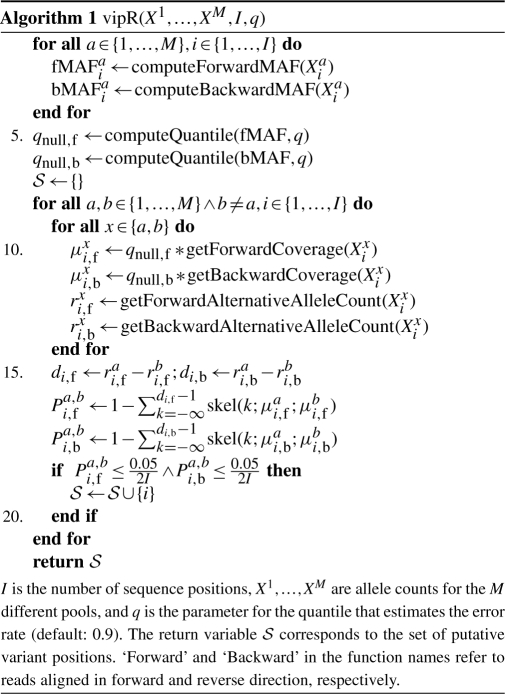
The pseudocode of the algorithm is given in Algorithm 1. Briefly, the first step is the computation of the alternative allele frequency. Next, the sequencing error rate is estimated as the q-th percent quantile of the alternative allele frequencies. This estimation is done separately for the reads aligned in forward and reverse direction. In the following, for simplicity, vipR utilizes only the frequency of the most frequent allele of all minor alleles. Using the error rate estimates, a one-sided P-value is computed based on the Skellam distribution for all possible pairs of pools. A position is considered a putative variant if the P-value for both directions of one pool-pair reaches below the Bonferroni corrected threshold of α=0.05/(2×I), where I is the number of sequence positions. In case the coverage of one strand is below a pre-defined threshold, a P-value below the threshold obtained on the other strand is sufficient (not displayed in the pseudo code). Finally, the set of putative variant positions is returned.

In a post-processing step, all putative variants are filtered with respect to the maximal observed frequency of the minor allele. More precisely, the filter removes positions at which the maximal MAF does not reach a specific threshold (default: 1/(1.5×h), with h being the number of haplotypes in the DNA pool). This criterion has to be met by the allele frequencies from both directions.

Error rates between base exchanges and small insertions and deletions may vary substantially within the same HTS platform. Thus, the screening for small deletions is carried out in a separate execution of the algorithm where a deletion is treated as a ‘fifth base’. The screening for small insertions, however, is currently not supported by vipR.

2.4 Sequence data

The sequencing data originates from a resequencing study of a total of 600 individuals. In all individuals, regions within TMEM132D on chromosome 12, which was found to be associated with panic disorder in a GWAS (Erhardt et al., 2010), were sequenced. The four DNA pools comprising 150 individuals each were generated using equimolar amounts of DNA from each individual. Two pools are control pools of healthy individuals, while the remaining two pools comprise only affected individuals (i.e. patients with panic disorder).

Eight target amplicons comprising the exonic regions of TMEM132D and covering a total 35.8 kb were amplified using specific primers and long-range PCR. The amplified DNA was prepared using the standard protocol for an ABI SOLiD fragment library with read length 50. One slide of the ABI SOLiD 3+ was partitioned into four equally sized compartments, and each pool was sequenced on such a single quad-slide resulting in ~82 million short reads per DNA pool.

As part of the quality control step, the reads were trimmed right before the fifth color of insufficient quality (quality value≤10). If the read comprised less than 30 colors after trimming, then it was discarded from further analysis. The remaining color reads were aligned in color space using BWA version 0.5.7 (Li and Durbin, 2009) to chromosome 12 of the human genome (NCBI Build 36.1) allowing a maximum of four color mismatches.

The numbers of short reads along the processing pipeline are summarized in Table 1. An average of 46.6 million reads per DNA pool could be used for variant detection. This amount corresponds to an approximate 50 000-fold coverage per base of the amplified region per DNA pool; hence a 160-fold coverage for each haplotype in the pool.

Table 1.

Number of HTS reads along the analysis pipeline

Pool name	Raw	After QC	For analysis
Cases 1	82.2	48.9	45.1
Cases 2	77.5	48.6	45.4
Controls 1	86.5	53.3	50.1
Controls 2	81.7	49.2	45.8

Numbers are given in millions. QC, quality control.

2.5 Statistical power calculation

As a first step, we compare the statistical power of the variant calling method based on the Skellam distribution with one based on the Poisson model. The power is studied in dependence of the coverage and other factors like sequencing error rate and allele frequency to be detected. The power calculation is based on the analysis presented by Out et al. (2009), which makes use of two different error rate estimates: the conservative estimate for the null hypothesis (i.e. no variant, just sequencing errors) is based on the 97.5th quantile of all MAFs (q_null=3.1×10⁻³). The second error rate estimate is based on the median (b=3×10⁻⁴), and is used together with the allele frequency to be detected f for modeling the fact that some erroneous reads of the major allele can contribute to a true sequence variant. Thus, the ratio for the alternative hypothesis is q_alt=f+b. The two ratios q_null and q_alt are multiplied with the coverage to yield λ_null and λ_alt, respectively. The use of two different error rate estimates prevents according to Out et al. (2009) false-positive detection of sequence variants in positions with high local error rate (by using a high q_null) and inflated power estimates (by using a moderate estimate of b).

Hence, in our analysis we first estimate the sequencing error rate from the data as the 90th percentile of all MAFs: q_null=2.7×10⁻³. Second, in concordance with Out et al. (2009), the error rate for the alternative hypothesis (i.e. presence of a sequence variant) is estimated from the data as the median of the observed MAFs, hence: b=1.6×10⁻⁴. Again, the rate q_alt under the alternative hypothesis is the sum of the frequency of the minor allele to be detected f and the error rate b: q_alt=f+b.

In the power calculation, we keep b fixed, but study the behavior under different values of f and q_null. More precisely, we focus on values of f that represent rare variants in a pool of 150 diploid individuals.

2.6 Validation

For the validation of vipR, we focused on sequence positions that had been confirmed to carry variants with two different techniques. The first set (set1) comprised 22 putative variant positions, which had been identified using high resolution melting curve analysis (Wittwer et al., 2003) and then veryfied by genotyping in every individual using a MALDI (Matrix-Assisted-Laser-Desorption/Ionization) TOF (time of flight) mass spectrometer (MassArray® system, Sequenom Inc., San Diego, USA) for SNP detection. However, of these 22 positions, one position exhibited an extremely low coverage by HTS (below 500) and was therefore excluded from the analysis. Of the remaining 21 positions, 18 displayed an SNP in at least one of the four DNA pools.

The second set (set2) of SNPs was selected based on the variant calling results by earlier versions of vipR and the Poisson model on the HTS data. Those SNPs were validated using the MALDI-TOF mass spectrography technology. This second set comprised a total of 82 positions, with 47 carrying a SNP in at least one DNA pool.

The performance of vipR in identifying SNPs was compared with a Poisson-based variant as presented in Out et al. (2009), and two other algorithms: CRISP and VarScan (Koboldt et al., 2009). Of note, the Poisson model used the same thresholds and filters as vipR: the error rate was estimated using the 90th percent quantile, and for the required maximal MAF the default setting was used (resulting in ). Hence, the only difference between these two approaches was the underlying probability distribution. During this step of the validation, we focused on available algorithms that were compatible with the SAM-format (Li et al., 2009), a standard HTS output format. This ensured the compatibility of the algorithms to different HTS platforms.

For vipR, Poisson and CRISP only reads with a mapping quality of at least 20 were eligible for inclusion into the analysis. Furthermore, only nucleotides with a minimum quality of 10 were used for SNP calling. VarScan did not allow to set these quality thresholds on read and nucleotide basis, but facilitated filtering of sequence positions regarding their average mapping and base quality, respectively. Thus, we set those parameters to the default values, 20 for average mapping quality and 15 for average base quality. The minimum coverage required for variant calling was set to 5000 for all algorithms. Furthermore, the minimum variant allele frequency threshold for VarScan was set to , likewise for CRISP the number of haplotypes in each pool was set to 300. The remaining settings for VarScan and CRISP were left on default. The pileup files that were used as input to vipR, Poisson and VarScan were generated with SAMtools (Li et al., 2009), while the pileup file for CRISP was produced using CRISP's own tool. VarScan and Poisson were applied to each pool separately, while CRISP and vipR were applied to all four pools in parallel.

3 RESULTS

3.1 Statistical power calculation

Figure 1a depicts the statistical power of the Skellam and Poisson distributions given the fixed q_null of 2.7×10⁻³ but varying coverage and three different allele frequencies to be detected. The sawtooth pattern of the power functions for both distributions is a direct consequence of their discrete nature: for many coverage values, the significance level simply happens to be strictly smaller than α and therefore leading to a small loss of power. The three frequencies correspond to one, two and four heterozygous alleles in a pool of 150 individuals, respectively. For all examined allele frequencies, the Skellam model showed a higher power than the Poisson model. This effect was most pronounced when detecting a single heterozygous allele: the Skellam model reached of a power 1.0 around a coverage of 7000; at this point, the Poisson model exhibited only a power of around 0.25. The difference in power between the two models decreased with the allele frequency to be detected.

Fig. 1.

Statistical power of the Skellam and the Poisson distribution. (a) Statistical power of both models depending on the coverage with varying allele frequency and fixed error rate of 2.7×10⁻³. (b) Statistical power of both models depending on the coverage with varying error rate (noise) and fixed allele frequency of . (c) Statistical power on real data for the Skellam model (black solid line) using one controls and one cases pool and for the Poisson model separately on one cases (blue solid line) and one controls (orange dashed line) pool.

Figure 1b illustrates the power of the two models with a fixed allele frequency corresponding to one heterozygous allele and three different sequencing error rates (noise) ranging from one to five sequencing errors in 1000 bases. Again, the Skellam model outperformed the Poisson model. The difference was most prominent in the setting modeling the highest noise, where the Skellam model reached a power of 1.0 at a coverage of 10 000 and the Poisson model still showed a power very close to 0.0. At a noise level of 0.3%, the Poisson model showed a slow increase in power with increasing coverage, while the Skellam model reached full power at a coverage of 6000. For the lowest noise level, both models perform similarly well.

The power of the two models on real sequence data is shown in Figure 1c. The noise rates q_null and b were estimated from the data and set to the values described above. The frequency of the alternative allele to be detected was set to a single heterozygous allele, i.e. . The figure depicts only the first three of all eight amplified regions of TMEM132D. The power computation for the Skellam model was based on one cases pool and one controls pool, while the computations for the Poisson model were done separately for the two pools. For most sequence positions, the power of the Skellam model exceeded the value of the Poisson model, thereby suggesting a greater sensitivity for detecting a single heterozygous allele in a pool of 150 individuals.

3.2 Real data

In order to assess the quality of the HTS data, we compared the minor allele frequency (MAF) measured by MALDI-TOF and by HTS. Figure 2 depicts the scatter plots between the MAF determined by HTS and the validation technique only at the sites where actual variations were detected using the reference method (18 from set1 and 47 from set2). Correlations are shown for each DNA pool individually. In general, correlations on set1 were higher (r=0.97 to r=0.99) than correlations on set2(r=0.81 to r=0.94). Moreover, in set2 the correlation between HTS and MALDI-TOF is comparable in both rare (MAF<5%;r=0.45) and common variants (MAF≥5%;r=0.42). In set1, the correlation observed in common variants (r=0.92) is higher than in rare variants (r=0.43). Here, however, the correlation value for the common variants is only based on three different position. Noteworthy, the figure suggests that HTS may deviate from the MAF estimated by the validation method. For instance, in DNA pool Cases 1, MALDI-TOF observed a MAF of 3% while HTS reported a MAF close to 0%.

Fig. 2.

Scatter plot between MAFs obtained by HTS and MALDI-TOF. (a) SNPs from different validation sets are represented by different symbols, and allele frequencies in the different DNA pools are color coded. (b) Like (a) but zoomed in on allele frequencies below 0.05.

Table 2 lists the numbers of variants found in all four pools. Since the VarScan algorithm and the Poisson model were applied to each pool individually, precise figures for each pool are provided. Both VarScan and CRISP identified in the 35 800 base pair region well above 9400 SNPs, i.e. almost one SNP every four base pairs among 600 individuals. The Poisson model and vipR detected much fewer variants in the same region with 1223 and 371 SNPs, respectively. Furthermore, the pool-wise listing reveals that the Poisson model detected one order of magnitude with fewer SNPs per pool than VarScan.

Table 2.

Number of variant positions found in each pool

	Cases 1	Cases 2	Controls 1	Controls 2	Total
vipR			–		371
CRISP			–		9425
Poisson	656	644	701	606	1223
VarScan	6711	6993	7582	6715	9856
vipR			–		56
CRISP			–		29
Poisson	31	31	33	28	42
VarScan	63	54	75	64	100

The upper part of the table lists the number of SNPs found in the resequenced region. The lower part lists the number of small deletions identified in the same region.

All algorithms detected by far fewer deletions than SNPs. The detected deletions had at most a length of four nucleotides (which was the maximum given the used alignment settings). CRISP detected the fewest number of deletions while VarScan detected the highest number. The relation of amount of deletions detected per pool and the amount of overall detected deletion for the Poisson model and VarScan, suggest a large overlap of deletions found in all four pools.

Figure 3 depicts the runtime behavior of all four tested algorithms on a single Intel core at 2.67 GHz (and 6 GB memory). The reported times comprise the computational time required for producing the output file starting from a pileup file, i.e. the generation of the pileup file was not part of the performance assessment. As expected, for the two programs that analyze DNA pools independently the runtime grows linearly with the increasing number of pools. The more interesting case concerns the tools that analyze the DNA pools in parallel. Here, vipR clearly outperforms CRISP: where CRISP ranges from 1.5 days for two pools to 9.5 days for all four pools, vipR requires only ≈20 min for all four pools. Remarkably, vipR was even quicker than Poisson. This fact, however, was mainly caused by longer output files generated by the Poisson model (comprising on average 650 SNPs versus 371 SNPs with vipR; Table 2). Moreover, the majority of time for vipR and Poisson was required during the pre-processing step (indicated by the difference between dashed and solid lines in Fig. 3).

Fig. 3.

Runtime of variant calling algorithms on the TMEM132D dataset in dependence of the number of pools. Time was measured in seconds and assessed on a single Intel core at 2.67 GHz (and 6 GB memory).

Of the 18 SNPs initially identified by melting curve analysis (set1), the Poisson model missed five, and falsely predicted one sequence position to be an SNP. On the same set, vipR showed a slightly better performance, and missed only three SNPs (of which two were also missed by the Poisson model), and also wrongly predicted the same sequence position as the Poisson model to be variant. CRISP missed only two SNPs and falsely predicted the same position as vipR and the Poisson model to be variant. The highest accuracy was achieved by VarScan, which missed only one SNP and falsely predicted the very same position as the other methods to be a variant. Summarizing, on this small set VarScan reached an accuracy of 90%, CRISP 86%, vipR showed an accuracy of 81% while the Poisson model yields an accuracy of 71%.

Of the 82 putative variant positions that were individually genotyped using MALDI-TOF mass spectrography (set2), 47 turned out to carry an alternative allele in at least one of the four DNA pools. Table 3 shows the performance of all four tools with respect to these 82 positions. Among the four tools, vipR showed the highest accuracy in classifying positions as variant or non-variant. CRISP performed slightly worse than vipR. The Poisson model and VarScan performed equally bad with respect to accuracy. The further performance measures sensitivity, specificity and precision afforded a more fine-grained evaluation of the four tools. As can be seen from Table 2, VarScan predicted many positions to be variant. Thus, in this set of 82 positions only 11 were predicted not to carry a variant. Consequently, VarScan achieved a high sensitivity but a very low specificity. CRISP and vipR showed a very similar sensitivity, but vipR outperformed CRISP clearly in both, specificity and precision. The Poisson model showed the lowest sensitivity. Interestingly, vipR and CRISP shared five positions predicted falsely to not carry a variant.

Table 3.

Performance on 82 validated variant positions of set2

	TP	FP	TN	FN	Accuracy	Sensitivity	Specificity	Precision
vipR	39	11	24	8	0.77	0.83	0.69	0.78
CRISP	40	15	20	7	0.73	0.85	0.57	0.73
Poisson	30	14	21	17	0.62	0.64	0.60	0.68
VarScan	43	28	7	4	0.61	0.91	0.20	0.61

P, positives; N, negatives; TP, true positives; FP, false positives; TN, true negatives; FN, false negatives. accuracy, ; sensitivity, ; specificity, ; precision, .

As many of the validated positions were actual rare variants with at most two heterozygous alleles (31 of 47 SNPs), it was unlikely that an SNP appeared in all four pools. Hence, a false-positive signal from one pool was likely to decrease the estimated specificity of the method when assessed in a position-wise setting. Moreover, for follow-up experiments it is often crucial to identify the DNA pool that is carrying the variant allele. Thus, in addition to analyzing the performance of the variant identification methods on the validated sequence positions across all pools, the performance was also assessed poolwise. For Poisson and VarScan, which analyzed the data for each pool independently, this could be carried out directly from the generated data. For CRISP and vipR the information of which pools contain the variant had to be manually inferred based on the observed MAFs and the information on the number of pools in which the variant was detected (CRISP) or the pools with significant P-values (vipR). Table 4 lists all three performance measures for each DNA pool separately. The values in row entitled ‘total’ are based on the sum of the confusion matrices of all four pools, i.e. these values are based on 328(=4·82) events as opposed to just 82.

Table 4.

DNA pool-wise performance on validated variant positions of set2

	Sensitivity				Specificity				Precision
	vipR	CRISP	Poisson	VarScan	vipR	CRISP	Poisson	VarScan	vipR	CRISP	Poisson	VarScan
Cases 1	0.77	0.77	0.72	0.81	0.89	0.79	0.89	0.59	0.77	0.63	0.75	0.48
Cases 2	0.76	0.76	0.52	0.72	0.91	0.75	0.79	0.53	0.81	0.63	0.58	0.46
Controls 1	0.81	0.81	0.56	0.85	0.95	0.75	0.89	0.55	0.88	0.61	0.71	0.48
Controls 2	0.88	0.88	0.72	0.92	0.95	0.72	0.88	0.54	0.88	0.58	0.72	0.47
Total	0.80	0.80	0.60	0.82	0.92	0.75	0.86	0.55	0.83	0.61	0.68	0.47

See description of Table 3.

As may be expected from the large number of identified SNPs by VarScan, its sensitivity was highest among the tested methods, but at the lowest observed specificity and precision. The Poisson model improved slightly in precision and substantially in specificity over VarScan, at a cost of a substantially decreased sensitivity. The sensitivity of CRISP and vipR was similar to the one obtained by VarScan, both methods, however, achieved far better specificity and precision values. Moreover, vipR clearly outperformed CRISP in specificity (0.92 versus 0.75) and precision (0.83 versus 0.61). Compared with the analysis by putative variant position, the individual analysis for every pool greatly improved the estimated specificity of all methods.

4 DISCUSSION

The power calculation for the Poisson distribution and the Skellam distribution demonstrated a clear advantage in favor of the Skellam distribution. For the given task, the Skellam distribution appeared to be much less susceptible to changes in the sequencing error rate (i.e. noise) than the Poisson distribution. Hence, it appears to be a suitable candidate for detecting differences in allele frequencies in multiple DNA pools and thereby identify sequence variants.

The advantage in statistical power on simulated data was confirmed on sequence data and based on real coverage values, an error rate estimated from that data, and the aim to detect a single heterozygous allele in 150 individuals. In most of the sequenced regions, the Skellam distribution exhibited a clearly higher power than the Poisson distribution, thus again suggesting a greater sensitivity in discovering real sequence variants.

The observed theoretical increase of sensitivity of the Skellam distribution over the Poisson distribution was substantiated on SNPs validated with two different techniques. More precisely, vipR yielded a 0.20 [0.19] increase in sensitivity over the Poisson model (at even slightly improved specificity) when SNPs in a single pool [sequence positions over all four pools] were used for performance calculation (Tables 3 and 4). Of note, since all remaining parameters were unchanged, the observed improvement in performance was only due to the exchange of the distribution function (and consequently the consideration of multiple DNA pools in parallel).

When comparing the MAF obtained from the results of HTS and the two reference methods, it appeared that while the overall correlation was good (r>0.80), the MAFs of specific positions may show large discrepancies and HTS sometimes seemed to grossly deviate from the allele frequency estimated by the validation techniques; sometimes overestimating and on other cases underestimating the MAF. On the other hand, the MAF estimated by individual genotyping might have also deviated from the true MAF as sometimes the genotyping was not successful in all 150 individuals. Unsuccessful genotyping is more likely to affect the performance assessment for variants with a very low MAF: if the validation technique fails to genotype the single individual with one heterozygous allele in the pool of 150 individuals, then one might consider a sequence variant called from the HTS data of that DNA pool as a false positive. On the other hand, the estimated MAF for SNPs with higher MAFs are less likely to be affected by failed genotyping, and here the observed discrepancy is due to shortcomings of HTS alone. A potential confounder of estimated MAF by HTS might also be extreme variations in coverage at these sequence positions. Thus, we examined the coverage at positions that exhibited more than 10% difference in MAF (corresponding to eight different sequence positions), but could not detect any correlations of MAF discrepancies and coverage. Interestingly, sequence positions with a large discrepancy in estimated MAF were often shared between pools.

Regarding the amount of sequence variants found by the algorithms, both VarScan and CRISP found well above 9400 variants, corresponding to roughly one variant every four bases. This value exceeds the expected number of one variant in 150 bases [roughly 15 million SNPs on 2.3 GB of accessed human genome; see Durbin et al. (2010)] by almost two orders of magnitude. This high number of putative variants was surprising, especially, as the sequenced regions covered the exonic regions of TMEM132D. The Poisson model retrieved almost one order of magnitude fewer variants from the same region, still corresponding to about one variant every 30 bases. Replacing the Poisson distribution with the Skellam distribution yielded 371 variants (roughly 1 variant every 95 bases). Despite the much smaller number of detected variants, vipR achieved a good sensitivity and specificity in identifying SNPs in the small test set of 82 putative SNPs. The remaining three methods demonstrated a considerably higher false-positive rate. However, a limitation of the performance assessment on set2 is the selection process of the putative variants: variants validated with MALDI-TOF were not randomly sampled over the sequenced region but chosen based on the results of earlier versions of vipR and the Poisson model. In particular, the selection was focused on variants showing low MAF (i.e. rare variants), appearing in interesting regions (exons and transcription factor binding sites) or showing a large difference in the allele count between cases and controls. Hence, the selection process was likely to introduce a bias in the measured performance. For instance, based on the raw numbers of identified SNPs, one can assume that the actual specificity of CRISP and VarScan is lower than the one estimated from the data. Moreover, methods that mark one-fourth of the sequenced region as sequence variants are not valuable for follow-up studies.

In contrast to the sequence variants of set2, the variants in set1 were selected prior to sequencing using HTS and therefore represent a set of SNPs that is not biased toward any of the four methods. The downside of set1 is that only 5 of the 18 validated SNPs were rare SNPs. Moreover, there were only three invalidated SNPs. Consequently, this set affords only a limited assessment of the algorithms' specificity and capability of detecting rare variants. The variants from set2 are by far better suited for this task.

A clear drawback of vipR over the Poisson model and VarScan is the requirement for more than one DNA pool in order to facilitate screening for sequence variants. However, when performing studies comprising a large number of individuals, distributing the individuals over multiple DNA pools is a necessity for generating sequence data of sufficient quality for detecting rare mutations. Altering the problem from discriminating real variants from sequencing errors to finding differences in allele frequencies across all pools is unlikely to affect the results negatively. In general there are two possibilities: (i) a sequence variant is frequent, then deviations of the allele count across the available pools are very likely; (ii) a sequence variant is rare, then it is unlikely, that the variant appears in all tested pools. Clearly, in the second scenario, using more pools decreases the risk of missing a real rare sequence variant.

Since the current implementation of vipR makes comparisons for each pair of DNA pools, a further drawback might occur when working with a large number of pools: the runtime will quickly increase. In this case, one could limit the number of comparisons by randomly selecting for each pool a fixed number of reference pools. It is unclear, however, how this heuristic would affect the results.

Last but not least vipR was the fastest tool to examine all four DNA pools for variants and clearly outperforming CRISP, which follows a similar strategy in identifying SNPs.

5 CONCLUSION

We presented vipR, a tool for variant detection in DNA pools that uses sequence information from multiple sequenced DNA pools in parallel for improving the sensitivity of variant detection. In our evaluation, vipR performed with the highest specificity and precision at a sensitivity superior to a Poisson-based model and comparable to two more methods. Moreover, vipR was the fastest tool among the evaluated methods; just requiring ≈20 min for all four DNA pools, opposed to ≈9.5 days required by CRISP the slowest tool. The source code of vipR can be obtained via http://sourceforge.net/projects/htsvipr/.

Conflict of Interest: none declared.

REFERENCES

- Bansal V. A statistical method for the detection of variants from next-generation resequencing of DNA pools. Bioinformatics. 2010;26:i318–i324. doi: 10.1093/bioinformatics/btq214. [DOI] [PMC free article] [PubMed] [Google Scholar]
- Dalca A.V., Brudno M. Genome variation discovery with high-throughput sequencing data. Brief. Bioinformatics. 2010;11:3–14. doi: 10.1093/bib/bbp058. [DOI] [PubMed] [Google Scholar]
- Dohm J.C., et al. Substantial biases in ultra-short read data sets from high-throughput DNA sequencing. Nucleic Acids Res. 2008;36:e105. doi: 10.1093/nar/gkn425. [DOI] [PMC free article] [PubMed] [Google Scholar]
- Druley T.E., et al. Quantification of rare allelic variants from pooled genomic DNA. Nat. Methods. 2009;6:263–265. doi: 10.1038/nmeth.1307. [DOI] [PMC free article] [PubMed] [Google Scholar]
- Durbin R.M., et al. A map of human genome variation from population-scale sequencing. Nature. 2010;467:1061–1073. doi: 10.1038/nature09534. [DOI] [PMC free article] [PubMed] [Google Scholar]
- Erhardt A., et al. TMEM132D, a new candidate for anxiety phenotypes: evidence from human and mouse studies. Mol. Psychiatry. 2010 doi: 10.1038/mp.2010.41. [Epub ahead of print; doi: 10.1038/mp.2010.41] [DOI] [PubMed] [Google Scholar]
- Koboldt D.C., et al. VarScan: variant detection in massively parallel sequencing of individual and pooled samples. Bioinformatics. 2009;25:2283–2285. doi: 10.1093/bioinformatics/btp373. [DOI] [PMC free article] [PubMed] [Google Scholar]
- Li H., Durbin R. Fast and accurate short read alignment with burrows-wheeler transform. Bioinformatics. 2009;25:1754–1760. doi: 10.1093/bioinformatics/btp324. [DOI] [PMC free article] [PubMed] [Google Scholar]
- Li H., et al. Mapping short DNA sequencing reads and calling variants using mapping quality scores. Genome Res. 2008;18:1851–1858. doi: 10.1101/gr.078212.108. [DOI] [PMC free article] [PubMed] [Google Scholar]
- Li H., et al. The sequence alignment/map format and samtools. Bioinformatics. 2009;25:2078–2079. doi: 10.1093/bioinformatics/btp352. [DOI] [PMC free article] [PubMed] [Google Scholar]
- Maher B. Personal genomes: the case of the missing heritability. Nature. 2008;456:18–21. doi: 10.1038/456018a. [DOI] [PubMed] [Google Scholar]
- Manolio T.A., et al. Finding the missing heritability of complex diseases. Nature. 2009;461:747–753. doi: 10.1038/nature08494. [DOI] [PMC free article] [PubMed] [Google Scholar]
- Out A.A., et al. Deep sequencing to reveal new variants in pooled DNA samples. Hum. Mutat. 2009;30:1703–1712. doi: 10.1002/humu.21122. [DOI] [PubMed] [Google Scholar]
- R Development Core Team. R Foundation for Statistical Computing. Vienna, Austria: 2008. R: A language and environment for statistical computing. [Google Scholar]
- Shendure J., Ji H. Next-generation DNA sequencing. Nat. Biotechnol. 2008;26:1135–1145. doi: 10.1038/nbt1486. [DOI] [PubMed] [Google Scholar]
- Skellam J. The frequency distribution of the difference between two Poisson variates belonging to different populations. J. R. Stat. Soc. Ser. A. 1946;109:296. [PubMed] [Google Scholar]
- Stratton M. Genome resequencing and genetic variation. Nat. Biotechnol. 2008;26:65–66. doi: 10.1038/nbt0108-65. [DOI] [PubMed] [Google Scholar]
- Visscher P.M., et al. Heritability in the genomics era–concepts and misconceptions. Nat. Rev. Genet. 2008;9:255–266. doi: 10.1038/nrg2322. [DOI] [PubMed] [Google Scholar]
- Wang C., et al. Characterization of mutation spectra with ultra-deep pyrosequencing: application to HIV-1 drug resistance. Genome Res. 2007;17:1195–1201. doi: 10.1101/gr.6468307. [DOI] [PMC free article] [PubMed] [Google Scholar]
- Watson G. A Treatise on the Theory of Bessel Functions. Cambridge: Cambridge University Press; 1995. [Google Scholar]
- Wittwer C.T., et al. High-resolution genotyping by amplicon melting analysis using LCGreen. Clin. Chem. 2003;49(6 Pt 1):853–860. doi: 10.1373/49.6.853. [DOI] [PubMed] [Google Scholar]
- Yi X., et al. Sequencing of 50 human exomes reveals adaptation to high altitude. Science. 2010;329:75–78. doi: 10.1126/science.1190371. [DOI] [PMC free article] [PubMed] [Google Scholar]