Abstract
Purpose: Classification of magnetic resonance (MR) images has many clinical and research applications. Because of multiple factors such as noise, intensity inhomogeneity, and partial volume effects, MR image classification can be challenging. Noise in MRI can cause the classified regions to become disconnected. Partial volume effects make the assignment of a single class to one region difficult. Because of intensity inhomogeneity, the intensity of the same tissue can vary with respect to the location of the tissue within the same image. The conventional “hard” classification method restricts each pixel exclusively to one class and often results in crisp results. Fuzzy C-mean (FCM) classification or “soft” segmentation has been extensively applied to MR images, in which pixels are partially classified into multiple classes using varying memberships to the classes. Standard FCM, however, is sensitive to noise and cannot effectively compensate for intensity inhomogeneities. This paper presents a method to obtain accurate MR brain classification using a modified multiscale and multiblock FCM.
Methods: An automatic, multiscale and multiblock fuzzy C-means (MsbFCM) classification method with MR intensity correction is presented in this paper. We use a bilateral filter to process MR images and to build a multiscale image series by increasing the standard deviation of spatial function and by reducing the standard deviation of range function. At each scale, we separate the image into multiple blocks and for every block a multiscale fuzzy C-means classification method is applied along the scales from the coarse to fine levels in order to overcome the effect of intensity inhomogeneity. The result from a coarse scale supervises the classification in the next fine scale. The classification method is tested with noisy MR images with intensity inhomogeneity.
Results: Our method was compared with the conventional FCM, a modified FCM (MFCM) and multiscale FCM (MsFCM) method. Validation studies were performed on synthesized images with various contrasts, on the simulated brain MR database, and on real MR images. Our MsbFCM method consistently performed better than the conventional FCM, MFCM, and MsFCM methods. The MsbFCM method achieved an overlap ratio of 91% or higher. Experimental results using real MR images demonstrate the effectiveness of the proposed method. Our MsbFCM classification method is accurate and robust for various MR images.
Conclusions: As our classification method did not assume a Gaussian distribution of tissue intensity, it could be used on other image data for tissue classification and quantification. The automatic classification method can provide a useful quantification tool in neuroimaging and other applications.
Keywords: magnetic resonance images (MRI), image classification, fuzzy C-means (FCM), bilateral filter, multiscale, multiblock
INTRODUCTION
Many clinical and research applications using magnetic resonance (MR) images require image classification. Unfortunately, classification of MR images can be challenging because MR images are affected by multiple factors such as noise, intensity inhomogeneity, and partial volume effects. Noise in MR images can cause classified regions to become disconnected. Partial volume effects occur where pixels contain a mixture of multiple tissue types, which makes the assignment of a single class to these boundary regions difficult. Intensity inhomogeneity in MR images manifests itself as a smooth intensity variation across the image. Because of this phenomenon, the intensity of the same tissue can vary with respect to the location of the tissue within the image. The conventional “hard” classification method restricts each pixel exclusively to one class and often results in crisp results. Fuzzy C-mean (FCM) classification or “soft” segmentation has been extensively applied to MR images, in which pixels are partially classified into multiple classes using varying memberships to the classes. Standard FCM, however, is sensitive to noise and cannot effectively compensate for intensity inhomogeneities.
Although an intensity inhomogeneity is usually hardly noticeable to a human observer, many medical image analysis methods, such as segmentation, registration, and classification, can be sensitive to the spurious variations of image intensities. A number of methods for intensity inhomogeneity correction of MR images have been proposed in the past. The intensity inhomogeneity correction methods were categorized into the prospective and retrospective approach.1 The prospective methods are further classified into sub-categories that are based on phantoms, multicoils, and special sequences. The retrospective methods are further classified into filtering, surface fitting, segmentation, and histogram based.
First, statistical model-based methods have been used for quantification of brain tissues in MR images.2 These methods typically employ a Gaussian finite mixture model to estimate the class mixture of each pixel by trying to fit the image histogram. The intensity of a single tissue type is modeled as a Gaussian distribution and the classification problem is solved by an expectation-maximization (EM) algorithm.3 Markov random field (MRF) is developed to model the spatial correlation and used as prior information in the EM optimization.4, 5 However, it is difficult to estimate parameters for an MRF model from the images and these methods still belongs to “hard” segmentation. Fuzzy classification normally refers to partial volume (PV) segmentation. Van et al. performed PV segmentation under EM-MRF framework,6 where each voxel consists of several different tissue types with different memberships.
FCM classification methods employ fuzzy partitioning to allow one pixel to be assigned to tissue types with different memberships graded between 0 and 1.7 FCM is an unsupervised algorithm and allows soft classification of each pixel which can consist of several different tissue types.8 Although the conventional FCM algorithm works well on most noise-free images, it does not incorporate spatial correlation information, which makes it sensitive to noise and MR inhomogeneity. Different modified FCMs have been proposed to compensate for field inhomogeneity and incorporate the spatial information.9 A regularization term10 was introduced into the conventional FCM cost function in order to impose the neighborhood effect. A geometry-guided FCM (GC-FCM) method was proposed,11 which incorporates geometrical condition information of each pixel and its relationship with its local neighborhood into the classification. Recently, some approaches directly add regularization terms to the objective function and show increased robustness for classification of MR images with intensity inhomogeneity.12 Inspired by the Markov random field and expectation-maximization algorithm,7 various modified FCM methods were proposed by incorporating different regularization terms to overcome the problem of being sensitive to noise.13, 14 Pham and Prince used a modified FCM cost function to model the variation in intensity values via a multiplicative bias field applied to the cluster centroids.8 As the performance of this method degrades significantly with increased noise, Li et al.15 modified the method and incorporated a noise suppression and inhomogeneity correction into the FCM framework. Based on a previously developed framework of fuzzy connectedness and object definition in multidimensional scenes,16 Saha et al. have proposed an extension of this framework that takes into account the local object size in defining connectedness.17, 18 By introducing an adaptive method to compute the weights of local spatial information in the objective function, the adaptive fuzzy clustering algorithm is capable of utilizing local contextual information to impose local spatial continuity, thus allowing the suppression of noise and helping to resolve classification ambiguity.19 In our previous study, a multiscale FCM (MsFCM) classification method for MR images was presented. 20 This method used a diffusion filter to process MR images and to construct a multiscale image series. The object function of the conventional FCM is modified to allow multiscale classification processing where the result from a coarse scale supervises the classification in the next fine scale.21 To address the effect of intensity inhomogeneity on image classification, we propose an automatic, multiscale and multiblock FCM (MsbFCM) classification method for MR images in this study. We construct multiscale, bilateral-filtered images by increasing the standard deviation of spatial function, and by reducing the standard deviation of range function. We separate every scale image into multiblock; the multiscale FCM classification method is applied in each block along the scales from the coarse to fine levels. Our MsbFCM method is described in Sec. 3.
MODEL OF INTENSITY INHOMOGENEITY
The task of MR image classification involves the separation of image voxels into regions comprising different tissue types. We assume that each tissue class has a specific value. Ideally, the signal would consist of piecewise constant regions. However, imperfection in the magnetic field often introduces an unwanted low frequency bias term into the signal, which gives rise to the intensity inhomogeneity.
The bias field that gives rise to the intensity inhomogeneity in an MR image is usually modeled as a smooth multiplicative field.8, 13, 22, 23, 24 The image formation process in MR imaging can be modeled as
| (1) |
where xi is the measured MR signal, yi is the true signal, bi is the unknown smoothly varying bias field, and ni is an additive noise assumed to be independent of bi. Accurate classification of an MR image thus involves determining an accurate estimation of the unknown bias field bi and noise ni, and then removing this bias field and noise from the measured MR signal.
METHOD
Conventional FCM method
The conventional FCM algorithm is an iterative method that produces an optimal c partition for the image by minimizing the weighted intergroup sum of squared error objective function JFCM
| (2) |
where is the characterized intensity center of the class k, and c is the number of underlying tissue types in the image which is given before classification. The uik represents the possibility of the voxel i belonging to the class k and it is required that uik∈[0,1] and for any voxel i. The parameter p is a weighting exponent on each fuzzy membership and it is set as 2.
Modified FCM (MFCM) method
A conventional FCM method only uses pixel intensity information and results in crisp segmentation for noisy images. In order to incorporate spatial information, different MFCM methods are proposed to allow the neighbors as factors to attract pixels into their cluster. An MFCM proposed by Ahmed has the following objective function12
| (3) |
where Ni stands for the neighboring pixels of the pixel i and NR is the total number of neighboring pixels, which is 8 for a 2D image and is 26 for a 3D volume. α controls the effect of the neighboring term and inversely proportional to the SNR of the MR signal.
MsFCM method based on anisotropic diffusion (AD) filtering
The above two FCM methods only use a single scale for classification and do not consider multiscale information. In our previous study, we developed a modified MsFCM method based on anisotropic diffusion (AD) filtering.20 The classification result at a coarser level l + 1 was used to initialize the classification at a higher scale level l. The final classification is the result at the scale level 0. The objective function of the MsFCM at the level l is described below.
| (4) |
Similarly, uik stands for the membership of the pixel i belonging to the class k, and vk is the vector of the center of the class k. xi represents the feature vectors from multiple weighted MR images, and Ni stands for the neighboring pixels of the pixel i. is the membership obtained from the classification in the previous scale. The objective function is the sum of three terms where α and β are scaling factors that define the effect of each factor term.
MsbFCM method with bias correction based on bilateral filtering
Since image classification algorithms can be sensitive to noise, image filtering can improve the performance of classification. Due to partial volume effect, MR images often have blurred edges. Linear filters can reduce noise but may result in the degradation of image contrast and detail.25, 26 Bilateral filtering can overcome this drawback by introducing a partial edge detection step into the filtering so as to encourage intraregion smoothing and preserve the interregion edge. A bilateral filter replaces the pixel value of a neighborhood center with the average of similar and nearby pixel values. In smooth regions, pixel values in a small neighborhood are similar to each other, and the bilateral filter acts essentially as a standard domain filter, averaging away the small, weakly correlated signal differences that were caused by noise.
Bilateral filtering was developed by Tomasi and Manduchias as an alternative to anisotropic diffusion.27, 28 It is a nonlinear filter where the output is a weighted average of the input. It starts with standard Gaussian filtering with a spatial kernel. However, the weight of a pixel also depends on a function in the intensity domain, which decreases the weight of pixels with large intensity differences. In practice, they use a Gaussian function in the spatial domain and another Gaussian function in the intensity domain. Therefore, the value at the pixel s is influenced mainly by pixels that are spatially close with a similar intensity. Durand and Dorsey have shown that 0-order anisotropic diffusion and bilateral filtering belong to the same family of estimators.28 However, anisotropic diffusion is adiabatic (energy-preserving), while bilateral filtering is not. In contrast to anisotropic diffusion, bilateral filtering does not rely on shock formation, so it is not prone to stair stepping.29, 30 Bilateral filtering is a particular choice of weights in the extended diffusion process that is obtained from geometrical considerations. In bilateral filtering, the kernel that plays the same role as the diffusion coefficient is extended to become globally dependent on intensity, whereas a gradient can only yield local dependency among neighboring pixels.31
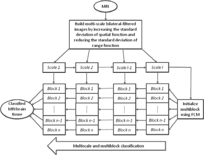
As modeled in Sec. 2, the bias field is seen as a smoothly varying multiplicative field. Although a bias field affects the intensity of different tissue in the whole image, it does not affect the relative intensity ratio of different tissue in a small region.1, 32, 33, 34 We divide the whole image into multiblocks and perform a multiscale classification in the small region. This can overcome the disadvantage of image classification algorithms that are sensitive to intensity inhomogeneity. Since the bias filed is a low frequency component it does not affect the relative intensity of different tissues within a small region. In order to reduce this effect by intensity inhomogeneity, an MR image is divided into many blocks as small as possible. On the other hand, a small block lacks global information so the block cannot be too small. Hence the size of the block will be determined in the multiblock strategy. When there is only one tissue in one block, we change the overlap rate of two neighbor blocks in order to make sure at least two tissues in one block. A schematic flow chart of our proposed algorithm for the MsbFCM method is shown in Fig. 1. We first use a mask for the brain in whole image. We use the top, bottom, left and right boundary lines. According to the size of the brain mask, we determine how many blocks for the classification. If the rectangle includes part of the tissue boundary, we will use the brain mask to select only the part inside the mask.
Figure 1.
Schematic flow chart of the proposed multiscale and multiblock FCM method.
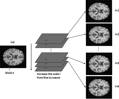
The multiscale space represents a series of images with different levels of spatial resolution. General information is extracted and maintained in large-scale images, and low-scale images have more local tissue information. Our multiscale description of images is generated by the bilateral filter. Figure 2 illustrates the scale space which was constructed using bilateral filtering.
Figure 2.
Multicale with multiblocks. The scale space is composed of a stack of the images filtered at different scales where l = 0 is the original image. Image at every scale is divided into blocks.
Bilateral filtering
Bilateral filter is a weighted average of the local neighborhood samples, where the weights are computed based on temporal and radiometric distance between the center sample and the neighboring samples.35 It smoothes images while preserving edges by means of a nonlinear combination of nearby image values.29 Bilateral filtering can be described as follows:
| (5) |
with the normalization that ensures that the weights for all the pixels add up to one.
| (6) |
where I(x) and h(x) denotes input and output images. Wσs measures the geometric closeness between the neighborhood center x and a nearby point ξ, and Wσr measures the photometric similarity between the pixel at the neighborhood center x and that of a nearby point ξ. Thus, the similarity function Wσr operates in the range of the image function I, while the closeness function Wσs operates in the domain of I.
A simple and important case of bilateral filtering is shift-invariant Gaussian filtering, in which both the spatial function Wσs and the range function Wσr are Gaussian functions of the Euclidean distance between their arguments. Wσs is described as:
| (7) |
where ds=∥ξ-x∥ is the Euclidean distance. The range function Wσr is analogous to Wσs:
| (8) |
where dr=|I(ξ)-I(x)| is a suitable measure of distance in the intensity space.
Multiscale space of bilateral filtering
When inputting a discrete image I, the goal of the multiscale bilateral decomposition36 is to first build a series of filtered images Il that preserve the strongest edges in I while smoothing small changes in intensity. Let the original image be the 0th scale (l=0) and set I0=I and then iteratively apply the bilateral filter to compute
| (9) |
with
| (10) |
where n is a pixel coordinate, Wσ(x)=exp(-x2∕σ2), σs,l and σr,l are the widths of the spatial and range Gaussians, respectively; and k is an offset relative to n that runs across the support of the spatial Gaussian. The repeated convolution by Wσs,l increases the spatial smoothing at each scale l; and we choose the σs,l so that the cumulative width of the spatial Gaussian doubles at each scale. At the finest scale, we set the spatial kernel σs,1=σs. Then we set σs,l=2μs(l-1)σs,l-1 for all l>1 and μs as the coefficient. The range Gaussian Wσr,l is an edge-stopping function. Ideally, if an edge is strong enough to survive after one iteration of the bilateral decomposition, we would like it to survive all subsequent iterations. To ensure this property we set σr,l=σr∕2μr(l-1) and μr as the coefficient. By reducing the width of the range Gaussian by a factor of 2μr(l-1) at every scale, we will reduce the chance that an edge that barely survives after one iteration will be smoothed away in later iterations.
Multiscale and multiblock FCM algorithm
After bilateral filtering processing, the MsbFCM algorithm performs classification from the coarsest to the finest scale, i.e., the original image. The classification result at a coarser level l + 1 was used to initialize the classification at a higher scale level l. The final classification is the result at the scale level 0. During the classification processing at the level l + 1, the pixels with the highest membership above a threshold are identified and assigned to the corresponding class. These pixels are labeled as training data for the next level l. The objective function of the MsbFCM at the level l and block n is
| (11) |
Similarly, nuik stands for the membership of the pixel i belonging to the class k in block n; and nvk is the vector of the center of the class k in block n. nxi represents the feature vectors in block n from multiweighted MR images, and Ni stands for the neighboring pixels of the pixel i. The objective function is the sum of three terms, where α and β are scaling factors that define the effect of each factor term. The first term is the object function used by the conventional FCM method which assigns a high membership to the voxel whose intensity is close to the center of the class. The second term allows the membership in neighborhood pixels to regulate the classification toward piecewise-homogeneous labeling. The third term is to incorporate the supervision information from the classification of the previous scale with that is determined as:
| (12) |
where γ is the threshold to determine the pixels with a known class in the next scale and is set as 0.85 in our implementation. The classification is implemented by minimizing the object function . The minimization of occurs when the first derivative of with respect to the nuik and nvk are zero, and the final classification and classes’ center are computed iteratively through these two necessary conditions. Taking the derivative of with respect to the nvk and setting the result to zero, the class center is updated according to Eq. 13. As long as , we used the Lagrangian method which converts this constraint optimization to an unconstraint problem. The membership nuik of every pixel i belongs to the class k, and is updated based on Eq. 14.
| (13) |
| (14) |
Classification evaluation
To evaluate the classification methods we used two overlap ratios between the classified results and the ground truth. The Dice overlap ratio is used for the classification evaluation. The Dice overlap ratio for each tissue type is computed as a relative index of the overlap between the ground truth A and the classification result B. It is defined as
| (15) |
At the same time, we define an error overlap ratio between the classified result and the ground truth for classification evaluation. The error overlap ratio is computed as an index of the overlap difference between the classification result and the ground truth. It is described as
| (16) |
where A and B are binary classified results from the ground truth and classification methods, respectively.
EXPERIMENT AND RESULTS
Our MsbFCM classification method has been evaluated by synthetic images and the McGill brain MR database.37, 38, 39 We also applied the method to classify real MR images and compared the classified results with the manual segmentation. Meanwhile, in order to compare the performance of these four fuzzy classification methods, FCM, MFCM, and MsFCM methods were applied to each dataset.
The four methods used a single set of parameters throughout the comparisons for the same data. Because our previous paper has discussed how to select parameters α, β, and λ,20 we selected the same values for comparison. For synthesized images, we set α=β=0.85 and Ni=8 for MFCM, MsFCM, and MsbFCM methods, and set the scale level as 6 for MsFCM and MsbFCM. The diffusion filter was used when diffusion constant was 15 and the step was 0.125, and the bilateral filter was performed when σs=1.2, σr=25, and μs=μr=0.5. Four blocks were used in our MsbFCM.
For simulated brain data and real data, we transformed the intensity of all images to the range of 0–255, and we only changed the diffusion constant of the diffusion filter to 150. We selected 16 blocks for our MsbFCM, and the other parameters with the same as those in the synthesized images.
Synthesized images
The synthetic images with three tissue types (labeled as Class 1, 2, and 3) are shown in Fig. 3a. In order to test the algorithm on images with poor contrast, we synthesized the images with different image quality. Image contrast (IC) is defined as the relative intensity difference between one class and its surroundings.
| (17) |
where Mb is the background intensity and Mt is the intensity of the tissue. We first give a preset intensity to the center sphere (Class 2) and define it as Mb. The intensities of Classes 1 and 3 are defined as Mt and are computed as Mt=Mb(1+IC) for Class 1 and Mt=Mb(1-IC) for Class 3 when a contrast is given. After the image is created, 10% Gaussian noise with a mean of 0 is added to the images to make SNR = 10, and the standard deviation of the added noise is 10% of the intensity of Class 1. Meanwhile, in order to simulate intensity inhomogeneity, we added a 35% linear bias field into the synthetic image. Here 35% indicates the difference between the maximum and minimum of the multiplied bias field. For a synthetic image with a bias field and noise, we multiplied the bias field, and then added the noise into it.
Figure 3.
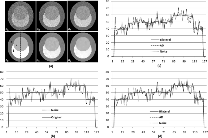
Bilateral and AD filter processing for a synthesized noisy image. (a) Image a1 is the original noisy image. a2 is the original image labeled with three classes (Class 1, 2, and 3). a3 and a5 are AD filtered results at scale 3 and scale 5, and a4 and a6 are bilateral filtered results at scale 3 and scale 5. (b) The signal profile along the center line of the noisy image and the original image without noise. (c) and (d) Signal profiles at the scales 3 (c) and 5 (d) of the original noisy image, with AD filtering, and with bilateral filtering, respectively.
The synthesized image has a size of 128×128 pixels. For five different intensities (Mb= 50, 80, 100, 120, and 150) and five different contrast (ICs = 10, 20, 30, 40, and 50%), a total of 25 images were synthesized to test the classification methods. For the four methods, MsbFCM, MsFCM, MFCM, and FCM, 100 classification experiments were performed on the synthesized images. The Dice and error overlap ratios of the classified results with the pre-efined truths were computed for each classification of each image.
Figure 3 demonstrates the effectiveness of the bilateral filtering process for the synthesized noisy image. In Fig. 3a a2, the synthesized image consists of three tissue types labeled as “Class 1”, “Class 2”, and “Class 3” with a given intensity, and a1 is a synthesized image with noise. a3 and a5 are filtered images after AD filtering processing at the scaled levels 3 and 5, and a4 and a6 are filtered images after bilateral filtering processing at the scaled levels 3 and 5. Figure 3b shows the intensity profile through the original synthesized image and noisy image. Figures 3c, 3d represent the intensity profile through the filtered images after bilateral and AD filtering processing at the scaled levels 3 and 5, respectively. As the scale increases, the noise is smoothed within each region, but the intensity difference at the edge has been enhanced so as to facilitate the classification. AD filtering can also reduce noise along scales, but bilateral filtering can denoise more under the same condition.
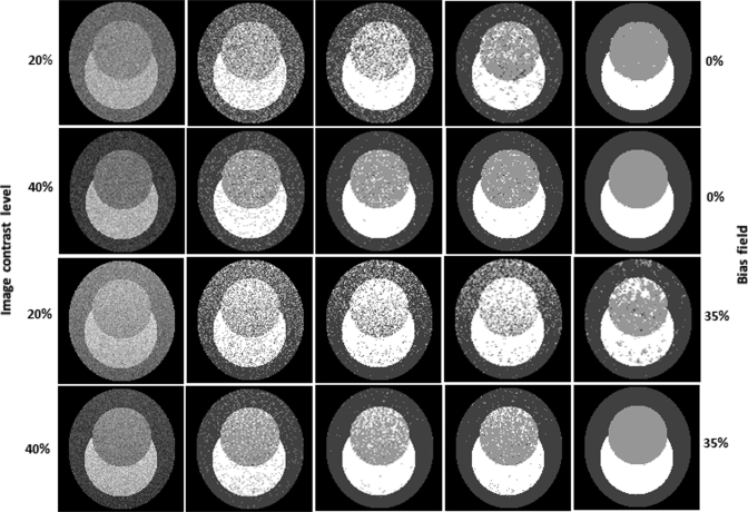
Figure 4 illustrates the visual assessment of the classification results on synthesized images and the comparison of the four methods. The synthesized images all have the same class distribution but with different image contrasts and intensity inhomogeneity. For the images with 40% image contrast and without intensity inhomogeneity, the four classification methods can successfully restore the class distribution, and the MFCM and MsFCM methods have more homogeneous results than the FCM approach. The MsbFCM can classify the three classes almost without errors. For the images with 40% image contrast and 35% intensity inhomogeneity, the classification results are almost same. For the images with 20% image contrast and no intensity inhomogeneity, the MsFCM and MsbFCM methods get better results than the FCM and MFCM, but the MsbFCM performs better than the MsFCM. In fact, the MsbFCM achieved acceptable results for images with 20% contrast and 35% intensity inhomogeneity while the other three methods failed. The MsbFCM method is robust for noise and intensity inhomogeneity.
Figure 4.
Comparison of the classification results using the four methods for synthesized images. The first column contains the original images with the designed contrast and bias level. The 2nd, 3rd, 4th, and 5th columns are the classification results using the FCM, MFCM, MsFCM and MsbFCM methods, respectively.
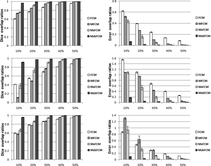
Figure 5 shows the Dice and error overlap ratios between the classification results and the ground truth for the three types of tissue (Class 1, 2, and 3) when synthesized images do not have intensity inhomogeneity. The Dice overlap ratios increase as the image contrast increases but the error ratios reduce. When the image contrast is higher than 40%, the four methods achieve accurate classification. When the contrast decreases, the performance of the FCM, MFCM and MsFCM decreases, but the MsbFCM method can still achieve high Dice overlap ratios of more than 90% and low error overlap ratios of less than 20%. The error bar represents the standard deviation of the Dice coefficients and error overlap ratios computed from the classification of the five images generated with a different mean intensity Mb and the same contrast.
Figure 5.
Quantitative evaluation of the classification results in synthesized images without bias field. Dice overlap ratios (Left) and error overlap ratios (Right) for Classes 1, 2, and 3 are shown from top to bottom, respectively. The Y axis is the overlap ratio between the ground truth and the classification results. The X-axis represents the contrast levels.
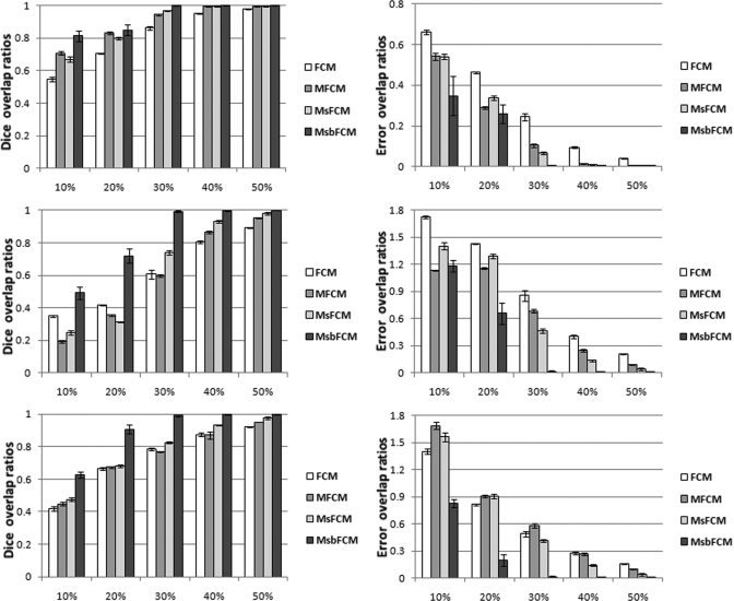
Figure 6 shows the Dice and error overlap ratios between the classification results and the ground truth for the three types of tissue (Class 1, 2, and 3) when synthesized images have 35% intensity inhomogeneity. When the image contrast is higher than 40%, the four methods achieve accurate classification. As the contrast decreases, the performance of the FCM, MFCM and MsFCM methods decreases, especially when the contrast is less than 30%. However, the MsbFCM method performs better than other three methods.
Figure 6.
Quantitative evaluation of the classification results in synthesized images with 35% bias field. Dice overlap ratios (Left) and error overlap ratios (Right) for Classes 1, 2, and 3 are shown from top to bottom, respectively. The Y axis is the overlap ratio between the ground truth and the classification results. The X-axis represents the contrast levels.
Simulated MR images
We obtained the brain MR images from the McGill phantom brain database for comprehensive validation of the classification methods. The MR volume was constructed by subsampling and averaging a high-resolution (1-mm isotropic voxels), low-noise dataset consisting of 27 aligned scans from one individual in stererotaxic space. The volume contains 181 × 217 × 181 voxels and covers the entire brain; the realistic brain phantom was then created from manual correction of an automatic classification of the MRI volume. An MR simulator is provided to generate specified MR images based on the realistic phantom. The MR tissue contrasts are produced by computing MR signal intensities from a mathematic simulation of the MR imaging physics. The MR images also take the effects of various image acquisition parameters, partial volume averaging, noise, and intensity nonuniformity into account.
Using the MR simulator, we obtained T1-weighted MR volumes with an isotropic voxel size of 1 mm and 20 and 40% intensity inhomogeneity at different noise percentages (0, 3, 5, 7, 9, and 15%). The noise effect was simulated as Gaussian noise adding to the MR volume with its standard deviation equal to the noise percentage multiplied by the brightest tissue intensity. The intensity inhomogeneity was implemented by multiplying the MR volume with a synthetic inhomogeneity field shape of the specified nonuniformity level. Prior to the classification, the extracranial tissues, such as skull, meninges, and blood vessels, had been removed manually so that the MR images for classification consisted of only three types of tissue, i.e., gray matter (GM), white matter (WM), and cerebrospinal fluid (CSF). The database also provides the ratio of each tissue type at each voxel and thus serves as the ground truth by assigning the voxel with the tissue type having the maximal ratio. We selected 2D transverse slices (Slices Nos. 70, 80, 90, 100, and 110) of the volumes with different noise levels for the classification evaluation. These MR images were used by the four classification methods.
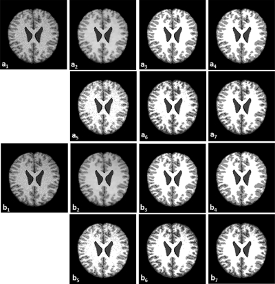
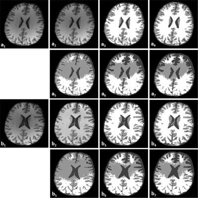
Figure 7 demonstrates the classification results on T1-weighted brain MR images with noise (9%) and intensity inhomogeneity (20 and 40%). Compared to the ground truth (a3 and b3), our MsbFCM method (a4 and b4) performed better than the FCM (a5 and b5), the MFCM (a6 and b6), and MsFCM (a7 and b7).
Figure 7.
Classification results of brain MR images with different intensity inhomogeneity. The original MR image with 9% noise and 20% intensity inhomogeneity (a1) and with 9% noise and 40% intensity inhomogeneity (b1) are smoothed after the bilateral filter processing (a2 and b2). a3 and b3 are the ground truth of the classification. a4 and b4, a5 and b5, a6 and b6, and a7 and b7 are the classification results using the MsbFCM, FCM, MFCM, and MsFCM methods, respectively.
The MsbFCM method was applied to the image with different noise levels. Tables Table I. and Table II. show the Dice overlap ratios for the different noise levels when intensity inhomogeneity is 20 and 40%, respectively. The overlap ratios are greater than 90 for 40% intensity inhomogeneity and 9% noise, indicating that the MsbFCM method is not sensitive to noise and intensity inhomogeneity.
Table 1.
Dice overlap ratios between the classification results and the ground truth for the brain data at different noise levels when intensity inhomogeneity is 20%.
| Noise | 0% | 3% | 5% | 7% | 9% |
|---|---|---|---|---|---|
| CSF | 0.97±0.00 | 0.96±0.01 | 0.94±0.01 | 0.92±0.01 | 0.90±0.01 |
| GM | 0.97±0.00 | 0.96±0.00 | 0.94±0.00 | 0.93±0.00 | 0.91±0.01 |
| WM | 0.98±0.01 | 0.97±0.01 | 0.96±0.01 | 0.95±0.01 | 0.94±0.01 |
Table 2.
Dice overlap ratios between the classification results and the ground truth for the brain data at different noise levels when intensity inhomogeneity is 40%.
| Noise | 0% | 3% | 5% | 7% | 9% |
|---|---|---|---|---|---|
| CSF | 0.95±0.01 | 0.94±0.01 | 0.93±0.01 | 0.92±0.01 | 0.91±0.01 |
| GM | 0.96±0.00 | 0.95±0.00 | 0.94±0.00 | 0.93±0.00 | 0.91±0.01 |
| WM | 0.97±0.01 | 0.97±0.01 | 0.96±0.01 | 0.95±0.01 | 0.94±0.02 |
We used both 20 and 40% bias fields with same bias distribution to simulate the 68% bias field. We applied the 68% bias field to original simulated MR images, and then added different noise (3, 5, 7, and 9% of max intensity). Table Table III. shows the Dice overlap ratios of three tissue types for different noise levels when intensity inhomogeneity is 68%. The overlap ratios of WM are greater than 90% for images with 68% intensity inhomogeneity and 9% noise.
Table 3.
The Dice overlap ratios between the classification results and the ground truth for the brain data at different noise levels when a 68% intensity inhomogeneity field is applied.
| Noise | 0% | 3% | 5% | 7% | 9% |
|---|---|---|---|---|---|
| CSF | 0.92±0.01 | 0.90±0.01 | 0.86±0.01 | 0.83±0.01 | 0.80±0.02 |
| GM | 0.92±0.01 | 0.90±0.01 | 0.86±0.01 | 0.82±0.01 | 0.78±0.02 |
| WM | 0.95±0.02 | 0.95±0.02 | 0.93±0.03 | 0.92±0.03 | 0.91±0.03 |
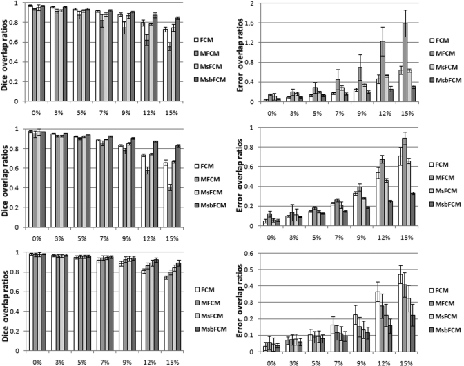
Figure 8 shows the comparison results of the four methods for the images at different noise levels. As the noise level increases, the Dice overlap ratios of the other three methods reduces observably and the error overlap ratios increase remarkably. However, the MsbFCM achieved a Dice ratio of (83 ± 1)% for the gray matter when the noise level is 15%. The MsbFCM method consistently performed better than the other three methods for different tissues and for images at different noise levels.
Figure 8.
Dice overlap ratios (Left) and error overlap ratios (Right) of the four methods, i.e., FCM, MFCM, MsFCM, and MsbFCM. The images were obtained from the McGill brain database with different noise and 20% intensity inhomogeneity. The results for CSF, GM, and WM are shown from top to bottom, respectively. The Y axis is the overlap ratio between the ground truth and the classification results. The X-axis represents noise levels.
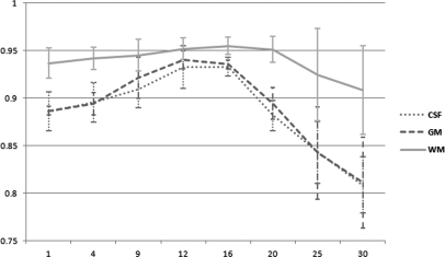
In order to evaluate how many rectangles would be optimal for segmenting patient data, we obtained T1-weighted MR volume with an isotropic voxel size of 1 mm and 40% intensity inhomogeneity at 5% noise. We selected five transverse slices from the volume to determine the number of blocks. Figure 9 shows the Dice overlap of three tissue types when different block numbers were used. There is no significant difference between 9 and 20 blocks for WM. For CSF and GM, the number between 12 and 16 works as well. For CSF, the standard deviation is larger when 12 blocks were used as compared to 16 blocks.
Figure 9.
Dice overlap ratios of three tissue types when different numbers of subblocks are used for the classification.
Real MR images
The four classification methods were applied to real T1-weighted MR images of the human brain. The MR images were acquired with a 4.0 Tesla MedSpec MRI scanner on a Siemens Syngo platform (Siemens Medical Systems, Erlangen, Germany). T1-weighted magnetization-prepared rapid gradient-echo sequence (MPRAGE) (TR = 2500 ms and TE = 3.73 ms) was used for the image acquisition. The volume has 256×256×176 voxels covering the whole brain yielding 1.0 mm isotropic resolution. Nonbrain structures such as the skull were manually removed. Manual segmentation of brain structures was performed in order to evaluate the classification. Two MR image slices were used to test the four classification methods.
Figure 10 illustrates the classification of the real MR brain data. Significant intensity inhomogeneity can be observed in the MR images. MsbFCM, FCM, MFCM, and MsFCM were performed on different slices. The MsbFCM performs better than FCM, MFCM, and MsFCM. The Dice overlap ratios are 92% for CSF, 84% for gray matter, and 94% for white matter.
Figure 10.
Classification of real brain MR images. a1 and b1 are the original MR images. a2 and b2 are the images after bilateral filtering. a3 and b3 are the classified results of the MsbFCM method. a4 and b4 are the manual segmentation results. a5 and b5, a6 and b6, and a7 and b7 are the classification results using the FCM, MFCM, and MsFCM methods, respectively.
DISCUSSION AND CONCLUSIONS
A multiscale and multiblock FCM classification method for MR images was developed and evaluated in this paper. We used a bilateral filter to effectively attenuate the noise within the images while preserving the edges between different tissue types. A scale space was generated by increasing the standard deviation of spatial function, by reducing the standard deviation of range function in the bilateral filter, and by keeping the general structure information in the images at a coarser scale. In order to reduce the effect of intensity inhomogeneity, we separate the image into multiblock. For every block, the classification was advanced along the scale space to include local information in the fine-level images. The result at a coarse scale provides the initial parameter for the classification in the next scale. Meanwhile, the pixels with a high probability of belonging to one class in the coarse scale will belong to the same class in the next level. Therefore, these pixels in the coarser scale are considered as pixels with a known class and are used as the training data to constrain the classification in the next scale. In this way, our MsbFCM method is not sensitive to noise and intensity inhomogeneity; and accurate classifications are obtained step-by-step. Using the multiscale and multiblock classification, higher spatial information is also included in the MsbFCM method. This approach can achieve a piecewise-homogeneous solution. Our method was evaluated using synthesized images, brain MR database, and real MR images. The classification method is accurate and robust for noisy images with intensity inhomogeneity.
The computation time can be improved in future implementation. We used five slices of the simulated volumes with 7% noise levels and 40% intensity inhomogeneity to evaluate classification time of the four methods. All the four methods are implemented in Matlab 2010a (MathWorks, Natick, MA) with a desk computer (Dell T7400, X5450*8 @ 3.0 GHz, 2.99 GHz, and 16 GB ram). The average time per slice for FCM, MFCM, MsFCM, and MsbFCM are 0.14±0.01 s, 50.96±5.50 s, 120.15±7.00 s and 180.76±5.21 s, respectively. The classification takes approximately 3 min that can be significantly reduced if C ++ and a high-performance workstation are used for the computation. Furthermore, multiscale classification for every block can be performed using a parallel framework to speed up the algorithm.
In this study, we reduced the effect of skull segmentation errors on classification by manually removing nonbrain structures such as the skull and scalp. In another report, we developed an automatic segmentation method for the skull on MR images,40 which allows us to automatically remove the skull from the brain MR images. In our segmentation-based attenuation correction methods for combined MR/PET,41, 42 we applied automatic skull segmentation to remove skull and use our classification to perform automatic classification. The multiscale and multiblock classification method can be applied to classify more than three tissue types. It can be used for classification of other MR images. The size of the block would need to be adjusted in order to fit into a specific application. Our method can be applied to 3D volume data. This could include more spatial regularization and lead to a better result. However, a fast 3D bilateral filtering algorithm is required. As our classification method did not assume a Gaussian distribution of tissue intensity, it could be used on other image data for tissue classification and quantification. We are integrating a quantitative image analysis package that combines our registration methods43, 44, 45 and classification methods, which can provide a useful tool in quantitative imaging applications.
ACKNOWLEDGMENTS
This research is supported in part by NIH grant R01CA156775 (PI: Fei), Coulter Translational Research Grant (PIs: Fei and Hu), Georgia Cancer Coalition Distinguished Clinicians and Scientists Award (PI: Fei), Emory Molecular and Translational Imaging Center (NIH P50CA128301), SPORE in Head and Neck Cancer (NIH P50CA128613), and Atlanta Clinical and Translational Science Institute (ACTSI) that is supported by the PHS Grant UL1 RR025008 from the Clinical and Translational Science Award program.
References
- Vovk U., Pernus F., and Likar B., “A Review of methods for correction of intensity inhomogeneity in MRI,” IEEE Trans. Med. Imaging 26, 405–421 (2007). 10.1109/TMI.2006.891486 [DOI] [PubMed] [Google Scholar]
- Cuadra M. B., Cammoun L., Butz T., Cuisenaire O., and Thiran J. P., “Comparison and validation of tissue modelization and statistical classification methods in T1-weighted MR brain images,” IEEE Trans Med. Imaging 24, 1548–1565 (2005). 10.1109/TMI.2005.857652 [DOI] [PubMed] [Google Scholar]
- Marroquin J. L., Vemuri B. C., Botello S., Calderon F., and Fernandez-Bouzas A., “An accurate and efficient Bayesian method for automatic segmentation of brain MRI,” IEEE Trans Med. Imaging 21, 934–945 (2002). 10.1109/TMI.2002.803119 [DOI] [PubMed] [Google Scholar]
- Held K., Kops E. R., Krause B. J., W. M.Wells, III, Kikinis R., and Muller-Gartner H. W., “Markov random field segmentation of brain MR images,” IEEE Trans Med. Imaging 16, 878–886 (1997). 10.1109/42.650883 [DOI] [PubMed] [Google Scholar]
- Zhang Y., Brady M., and Smith S., “Segmentation of brain MR images through a hidden Markov random field model and the expectation-maximization algorithm,” IEEE Trans Med. Imaging 20, 45–57 (2001). 10.1109/42.906424 [DOI] [PubMed] [Google Scholar]
- Van Leemput K., Maes F., Vandermeulen D., and Suetens P., “A unifying framework for partial volume segmentation of brain MR images,” IEEE Trans. Med. Imaging 22, 105–119 (2003). 10.1109/TMI.2002.806587 [DOI] [PubMed] [Google Scholar]
- Bezdek J., “A convergence theorem for the fuzzy ISODATA clustering algorithms,” IEEE Trans. Pattern Anal. Mach. Intell. 1–8 (1980). 10.1109/TPAMI.1980.4766964 [DOI] [PubMed] [Google Scholar]
- Pham D. L. and Prince J. L., “Adaptive fuzzy segmentation of magnetic resonance images,” IEEE Trans. Med. Imaging 18, 737–752 (1999). 10.1109/42.802752 [DOI] [PubMed] [Google Scholar]
- Tolias Y. A. and Panas S. M., “On applying spatial constraints in fuzzy image clustering using a fuzzy rule-based system,” IEEE Signal Process. Lett. 5, 245–247 (1998). 10.1109/97.720555 [DOI] [Google Scholar]
- Noordam J. C., Van den B., W. H. A. M, Buydens, and C L. M., “Geometrically guided fuzzy C-Means clustering for multivariate image segmentation,” Proceedings of the International Conference on Pattern Recognition, IEEE Computer Society, Barcelona, Spain, Vol. 1, pp. 462–465 (2000). 10.1109/ICPR.2000.905376 [DOI]
- Ahmed M. N., Yamany S. M., Mohamed N., Farag A. A., and Moriarty T., “A modified fuzzy C-means algorithm for bias field estimation and segmentation of MRI data,” IEEE Trans. Med. Imaging 21, 193–199 (2002). 10.1109/42.996338 [DOI] [PubMed] [Google Scholar]
- Kannan S. R., Ramathilagam S., Sathya A., and Pandiyarajan R., “Effective fuzzy C-means based kernel function in segmenting medical images,” Comput. Biol. Med. 40, 572–579 (2010). 10.1016/j.compbiomed.2010.04.001 [DOI] [PubMed] [Google Scholar]
- Liew A. W. and Yan H., “An adaptive spatial fuzzy clustering algorithm for 3D MR image segmentation,” IEEE Trans. Med. Imaging 22, 1063–1075 (2003). 10.1109/TMI.2003.816956 [DOI] [PubMed] [Google Scholar]
- Chen S. and Zhang D., “Robust image segmentation using FCM with spatial constraints based on new kernel-induced distance measure,” IEEE Trans. Syst., Man, Cybern., Part B: Cybern. 34, 1907–1916 (2004). 10.1109/TSMCB.2004.831165 [DOI] [PubMed] [Google Scholar]
- Li X., Li L., Lu H., and Liang Z., “Partial volume segmentation of brain magnetic resonance images based on maximum a posteriori probability,” Med. Phys. 32, 2337–2345 (2005). 10.1118/1.1944912 [DOI] [PMC free article] [PubMed] [Google Scholar]
- Udupa J. K. and Samarasekera S., “Fuzzy connectedness and object definition: Theory, algorithms, and applications in image segmentation,” Graphical Models Image Process. 58, 246–261 (1996). 10.1006/gmip.1996.0021 [DOI] [Google Scholar]
- Saha P. K., Udupa J. K., and Odhner D., “Scale-based fuzzy connected image segmentation: Theory, algorithms, and validation,” Comput. Vis. Image Underst. 77, 145–174 (2000). 10.1006/cviu.1999.0813 [DOI] [Google Scholar]
- Udupa J. K. and Saha P. K., “Fuzzy connectedness and image segmentation,” Proceedings of the IEEE, IEEE, New Jersey, Vol. 91, pp. 1649–1669 (2003). 10.1109/JPROC.2003.817883 [DOI]
- Ji Z. X., Sun Q. S., and Xia D. S., “A modified possibilistic fuzzy C-means clustering algorithm for bias field estimation and segmentation of brain MR image,” Comput. Med. Imaging Graph. (in press). [DOI] [PubMed]
- Wang H. and Fei B., “A modified fuzzy C-means classification method using a multiscale diffusion filtering scheme,” Med. Image Anal. 13, 193–202 (2009). 10.1016/j.media.2008.06.014 [DOI] [PMC free article] [PubMed] [Google Scholar]
- Wang H., Feyes D., Mulvihil J., Oleinick N., Maclennan G., and Fei B., “Multiscale fuzzy C-means image classification for multiple weighted MR images for the assessment of photodynamic therapy in mice,” Proc. SPIE, 6512, 65122W (2007). 10.1117/12.710188 [DOI] [PMC free article] [PubMed] [Google Scholar]
- Shattuck D. W., Sandor-Leahy S. R., Schaper K. A., Rottenberg D. A., and Leahy R. M., “Magnetic resonance image tissue classification using a partial volume model,” Neuroimage 13, 856–876 (2001). 10.1006/nimg.2000.0730 [DOI] [PubMed] [Google Scholar]
- Styner M., Brechbuhler C., Szekely G., and Gerig G., “Parametric estimate of intensity inhomogeneities applied to MRI,” IEEE Trans. Med. Imaging 19, 153–165 (2000). 10.1109/42.845174 [DOI] [PubMed] [Google Scholar]
- Meyer C. R., Bland P. H., and Pipe J., “Retrospective correction of intensity inhomogeneities in MRI,” IEEE Trans. Med. Imaging. 14, 36–41 (1995). 10.1109/42.370400 [DOI] [PubMed] [Google Scholar]
- Yang X. and Fei B., “A wavelet multiscale denoising algorithm for magnetic resonance (MR) images,” Meas. Sci. Technol. 22, 025803–025815 (2011). 10.1088/0957-0233/22/2/025803 [DOI] [PMC free article] [PubMed] [Google Scholar]
- Skiadopoulos S., Karatrantou A., Korfiatis P., Costaridou L., Vassilakos P., Apostolopoulos D., and Panayiotakis G., “Evaluating image denoising methods in myocardial perfusion single photon emission computed tomography (SPECT) imaging,” Meas. Sci. Technol. 20, 104023–104034 (2009). 10.1088/0957-0233/20/10/104023 [DOI] [Google Scholar]
- Tomasi C. and Manduchi R., “Bilateral filtering for gray and color images,” Computer Vision, ICCV ’98 Proceedings of the Sixth International Conference on Computer Vision, IEEE Computer Society, Washington, D.C. (1998) pp. 839–846.
- Durand F. and Dorsey J., “Fast bilateral filtering for the display of high-dynamic-range images,” ACM Trans. Graphics 21, 257–266 (2002). 10.1145/566654.566574 [DOI] [Google Scholar]
- Elad M., “On the origin of the bilateral filter and ways to improve it,” IEEE Trans. Med. Imaging 11, 1141–1151 (2002). 10.1109/TIP.2002.801126 [DOI] [PubMed] [Google Scholar]
- Barash D., “Bilateral filtering and anisotropic diffusion: Towards a Unified Viewpoint,” in Scale-Space and Morphology in Computer Vision, edited by Kerckhove M., Springer, Berlin/Heidelberg, 2006), Vol. 6, pp. 273–280. [Google Scholar]
- Barash D., “Fundamental relationship between bilateral filtering, adaptive smoothing, and the nonlinear diffusion equation,” IEEE Trans. Pattern Anal. Mach. Intell. 24, 844–847 (2002). 10.1109/TPAMI.2002.1008390 [DOI] [Google Scholar]
- Chang M. C. and Tao X., “Subvoxel segmentation and representation of brain cortex using fuzzy clustering and gradient vector diffusion,” Proc. SPIE 7623, 76231L.1–76231L.11 (2010). 10.1117/12.843853 [DOI] [Google Scholar]
- Manjon J. V., Lull J. J., Carbonell-Caballero J., Garcia-Marti G., Marti-Bonmati L., and Robles M., “A nonparametric MRI inhomogeneity correction method,” Med. Image Anal. 11, 336–345 (2007). 10.1016/j.media.2007.03.001 [DOI] [PubMed] [Google Scholar]
- Wang H., Das S., Pluta J., Craige C., Altinay M., Avants B., Weiner M., Mueller S., and Yushkevich P., “Standing on the shoulders of giants: Improving medical image segmentation via bias correction,” Med. Image Comput. Comput. Assist. Interv. 13, 105–112 (2010). 10.1007/978-3-642-15711-0_14 [DOI] [PMC free article] [PubMed] [Google Scholar]
- Yang X., Sechopoulos I., and Fei B., “Automatic tissue classification for high-resolution breast CT images based on bilateral filtering,” Proc. SPIE 7962, 79623H (2011). 10.1117/12.877881 [DOI] [PMC free article] [PubMed] [Google Scholar]
- Fattal R., Agrawala M., and Rusinkiewicz S., “Multiscale shape and detail enhancement from multi-light image collections,” ACM Trans. Graphics 26, 1–9 (2007). 10.1145/1276377.1276509 [DOI] [Google Scholar]
- Aubert-Broche B., Evans A. C., and Collins L., “A new improved version of the realistic digital brain phantom,” Neuroimage 32, 138–145 (2006). 10.1016/j.neuroimage.2006.03.052 [DOI] [PubMed] [Google Scholar]
- Kwan R. K. S., Evans A. C., and Pike G. B., “MRI simulation-based evaluation of image-processing and classification methods,” IEEE Trans. Med. Imaging 18, 1085–1097 (1999). 10.1109/42.816072 [DOI] [PubMed] [Google Scholar]
- Kwan R. K.-S., Evans A. C., and Pike G. B., “An extensible MRI simulator for post-processing evaluation,” in Proceedings of the 4th International Conference on Visualization in Biomedical Computing (Springer-Verlag, 1996) pp. 135–140.
- Yang X. and Fei B., “A skull segmentation method for brain MR images based on multiscale bilateral filtering scheme,” Proc. SPIE 76233, 76233K (2010). 10.1117/12.844677 [DOI] [Google Scholar]
- Fei B., Yang X., and Wang H., “An MRI-based attenuation correction method for combined PET/MRI applications,” Proc. SPIE 7262, 726208 (2009). 10.1117/12.813755 [DOI] [PMC free article] [PubMed] [Google Scholar]
- Fei B., Yang X., Nye J., Jones M., Aarsvold J., Raghunath N., Meltzer C., and Votaw J., “MRI-based attenuation correction and quantification tools for combined MRI/PET,” J. Nucl. Med. Meet. Abstr. 51, 81 (2010). 10.1117/12.813755 [DOI] [Google Scholar]
- Fei B., Duerk J. L., Sodee D. B., and Wilson D. L., “Semiautomatic nonrigid registration for the prostate and pelvic MR volumes,” Acad. Radiol. 12, 815–824 (2005). 10.1016/j.acra.2005.03.063 [DOI] [PubMed] [Google Scholar]
- Fei B., Lee Z., Duerk J. L., Lewin J. S., Sodee D. B., and Wilson D. L., “Registration and fusion of SPECT, high resolution MRI, and interventional MRI for thermal ablation of the prostate cancer,” IEEE Trans. Nucl. Sci. 51, 177–183 (2004). 10.1109/TNS.2003.823027 [DOI] [Google Scholar]
- Fei B., Wang H., R. F.Muzic, Jr., Flask C. A., Wilson D. L., Duerk J. L., Feyes D. K., and Oleinick N. L., “Deformable and rigid registration of MRI and microPET images for photodynamic therapy of cancer in mice,” Med. Phys. 33, 753–760 (2006). 10.1118/1.2163831 [DOI] [PubMed] [Google Scholar]


