A model of top-down gain control in the auditory system

Abstract

To evaluate a model of top-down gain control in the auditory system, 6 participants were asked to identify 1-kHz pure tones differing only in intensity. There were three 20-session conditions: (1) four soft tones (25, 30, 35, and 40 dB SPL) in the set; (2) those four soft tones plus a 50-dB SPL tone; and (3) the four soft tones plus an 80-dB SPL tone. The results were well described by a top-down, nonlinear gain-control system in which the amplifier’s gain depended on the highest intensity in the stimulus set. Individual participants’ identification judgments were generally compatible with an equal-variance signal-detection model in which the mean locations of the distribution of effects along the decision axis were determined by the operation of this nonlinear amplification system.

Behaviorally, the range of human hearing exceeds 100 dB, even though the range of intensities that can be encoded by any single primary auditory afferent is undoubtedly much smaller (see, e.g., Kiang, Watanabe, Thomas, & Clarke, 1965). One way to obtain a large behavioral response range despite the range limitations of primary auditory afferents is to assume the existence of an adjustable nonlinear amplification system that can control the dynamic range of hearing (Gordon & Schneider, 2007; Parker, Murphy, & Schneider, 2002; Parker & Schneider, 1994; Robles & Ruggero, 2001; Schneider & Parker, 1990; Yates, 1995). An appropriately designed gain-control mechanism, by expanding or compressing the sensory representation of stimuli to varying degrees, can serve two functions: (1) It can protect sensory systems from overload, and (2) it can enhance discriminability among selected stimuli.

A recent study (Taranda et al., 2009) supports the notion that compressing the response of the auditory system can prevent or reduce hearing loss following exposure to intense noise. These investigators genetically engineered a knockin mouse line in which the magnitude and duration of efferent cholinergic effects were magnified, thereby increasing the degree of efferent inhibition (suppression of distortion product otoacoustic emissions) by the olivocochlear bundle. Such mice proved to be more resistant to permanent threshold shifts induced by loud noises than were their wild-type counterparts. Because the olivocochlear bundle modulates the activity of outer hair cells, which in turn govern the amount of amplification in the cochlea, it appears that a gain-control mechanism that suppresses the response to high-intensity sounds has a valuable protective function in hearing.

This protection against overload could be provided by a linear or by a nonlinear gain-control system. All that would be needed is a system that turned down the gain (attenuated the auditory input) when the sound intensity increased. But Parker and Schneider (1994) have shown that a compressive nonlinear amplifier, in which the degree of compression is adjustable, could, in addition, provide enhanced discriminability in a targeted range—something that a linear system cannot easily do. Moreover, a nonlinear amplification system that was under top-down control, such that it could be modified by the expectations of listeners with regard to the sound intensities they were likely to experience, could both protect against sensory overload and maintain relatively good discriminative sensitivity. For example, in a loud noisy environment, the gain would be set to a low level to protect against overload. However, the gain should be set to high whenever the auditory environment is quiet (and expected to remain so) to enable the listener to hear and discriminate among soft sounds (e.g., listening to the movements of animals in the brush on a quiet day). A similar nonlinear mechanism has been shown to operate with respect to visual contrast (de la Rosa, Gordon, & Schneider, 2009; Mišić, Schneider, & McIntosh, 2010; Schneider, Parker, & Moraglia, 1996), suggesting that nonlinear gain-control mechanisms may be a common feature of sensory systems.

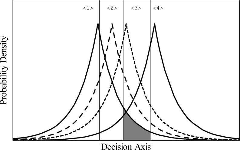
Parker et al. (2002) showed that a nonlinear gain-control mechanism was qualitatively consistent with participants’ performance in absolute identification (AI) of auditory intensities. In an AI task, a listener has to identify which of m possible stimuli was presented on a trial. For example, in the baseline condition in Parker et al., the possible stimuli consisted of four 1-kHz tones differing in intensity (25, 30, 35, and 40 dB SPL), and the participant was asked to specify which of the four had been presented on a trial by pressing one of four buttons. In a signal-detection analysis of an AI experiment, it is assumed that the presentation of stimulus j on a trial gives rise to a response effect along a decision axis. Because of variability either in the stimulus or in auditory processes, repeated presentations of stimulus j are assumed to give rise to a distribution of effects along the decision axis having some mean, μ, and standard deviation, σ. In the simplest models of this process, the shape of the distribution and its variance are assumed to be independent of stimulus magnitude. Figure 1 presents an example of how events along the decision axis might be distributed. In this model, the distributions of effects associated with a stimulus are Laplacian in shape and have equal variances. The observer is assumed to establish m - 1 criteria along this decision axis that divide it into m different response regions. When a stimulus is presented on a trial, it is assumed that if it evokes an effect in region k, the listener will identify it as tone k. Parker et al., as well as Gordon and Schneider (2007), found that the AI performance of a group of participants was quantitatively consistent with a model such as that shown in Fig. 1, in which the shape of the underlying distributions was Laplacian. In addition, the locations of the means of these distributions and how they changed with the intensity of the loudest stimulus in the set were qualitatively consistent with a model in which the internal representation of a stimulus along the decision axis was governed by a nonlinear gain-control mechanism.

Fig. 1.

The Laplace equal-variance model for a four-alternative absolute identification experiment. Each stimulus j, {1 ≤ j ≤ 4}, gives rise to a Laplace distribution of events along the decision axis. The vertical lines represent the criteria that divide the decision axis into k response regions {1 ≤ k ≤ 4} . The shaded portion is the probability that stimulus 1 will be misidentified as stimulus 3

The primary objective of the present investigation was to accumulate sufficient data on AI to determine whether a specific model of the nonlinear gain-control mechanism could predict both group and individual performance in quantitative detail (a detailed description of the model will be presented in connection with our data). A secondary objective was to compare predictions of the gain-control model with those of attention-allocation models (e.g., Luce & Green, 1978; Nosofsky & Luce, 1984). To do this, we needed to collect extensive data on individual participants so that we could examine, on an individual basis, how the intensity of the loudest stimulus in the set affected discriminability among the tones in the set and whether there were sequential dependencies in the data.

A third objective was to determine why participants’ decisions appeared to be based on the Laplace distribution in Parker et al. (2002) and Gordon and Schneider (2007), rather than on the normal distribution traditionally used in signal-detection theory. Schneider (2007) identified a possible reason for this. Using Monte Carlo techniques, he showed that group data will be well-fit by the Laplace equal-variance (LEV) model (illustrated in Fig. 1) even if every individual participant’s data are well-fit by the traditional Gaussian equal-variance (GEV) model if the value of the variance parameter in the GEV model differs substantially across individuals. Because group data were used in Parker et al. and in Gordon and Schneider, the better fit obtained for the Laplace distribution than for the normal distribution could be due to individual differences, rather than to underlying processes. A fourth objective was to see how participant performance would evolve over many sessions of the same AI task. Would performance improve, and would individual differences be stable over time?

To answer these questions, we had 6 individuals complete 20 sessions of AI in each of three conditions. In the first (baseline) condition, there were four low-intensity (25, 30, 35, and 40 dB SPL) 1-kHz pure tones in the set to identify. In the other two conditions, a fifth tone (either 50 or 80 dB SPL) was added to the baseline set. In all, each participant provided 60 sessions worth of data.

Method

Participants

Six students and staff members at the University of Toronto Mississauga (3 females, 3 males) served. Their ages ranged from 19 to 39 years. All reported normal hearing. Audiograms, which were available for 5 of the 6 participants, were all in the normal range. Each participant served in all parts of the study.

Apparatus and stimuli

The stimuli were 1-kHz tones with intensities of 25, 30, 35, 40, 50, and 80 dB SPL presented diotically via TDH-49P headphones to the participants, who were seated in a double-walled, sound-attenuating chamber. Tones were digitally generated at a rate of 20 kHz and were converted to voltages using a Tucker Davis Technologies (TDT) sound system II. All tones were produced with a 10-msec rise/fall time and were attenuated to the proper level by means of a TDT programmable attenuator. Tone durations were 500 ms.

Procedure

There were three conditions in the experiment:baseline (B), B + 50, and B + 80. The stimuli in the baseline condition were the 25-, 30-, 35-, and 40-dB SPL tones. The other two conditions included either a 50- (B + 50) or an 80- (B + 80) dB SPL tone in addition to the four used in the baseline condition. Those three conditions could be sequenced in any of six permutations. Each of those six permutations was used with 1 participant.

Participants were informed that they would be hearing a series of tones and that they were to identify those tones by pressing the button assigned to that tone on a button-box. The leftmost button was assigned to the softest tone, the next to the next-softest tone, …, and the rightmost button was assigned to the loudest tone. Only the four leftmost of the five buttons were available in the baseline condition, there being only four stimuli.

In each condition, each of the stimuli was presented 50 times in each session. Thus, there were 200 stimuli in a baseline session and 250 stimuli in a session of the other two conditions. Stimuli were presented in randomly sequenced blocks of 50. If, for any tone, the participant did not respond within 2.5 s of stimulus presentation, all previous data for that block were discarded, and the block began anew. Feedback was provided by a 200-ms flash of the light above the correct button once the participant had responded.

The subject initiated a session by pressing a Start button. Tones followed buttonpresses after 100 ms. Each session began with either 40 (baseline condition) or 50 (the other two conditions) practice trials, on which each stimulus was presented 10 times.

Participants served in 20 sessions in each of the three conditions, for a total of 60 sessions. After 20 sessions in the first condition, the participant began the second condition and, after that was completed, served in the third condition. Sessions lasted approximately 20 min in the baseline condition and 25 min in the other two conditions. Participants could and often did run in several sessions in a single day.

Results

For each of the three conditions (B, B + 50, and B + 80), the data from each participant were divided into four consecutive blocks, each consisting of five sessions. Because we were primarily interested in the degree to which the addition of a fifth stimulus (at either 50 or 80 dB SPL) would affect a listener’s ability to discriminate among the four base tones (25, 30, 35, and 40 dB SPL), a response on either button 4 or 5 when any of the four base tones were presented was scored as a button-4 response because, in a signal-detection analysis (see Fig. 1), a response on either of these two buttons, indicated that the participant classified the tone in question as being louder than the three lowest intensity tones in the baseline set (to the right of the criterion dividing response region 3 from response region 4 in Fig. 1).1 Hence, for each participant, the data consisted of four, 4 × 4 response-probability matrices (p[R _k|S _j], {1 ≤ k ≤ 4}, {1 ≤ j ≤ 4}) corresponding to the four blocks of sessions, where S _j is stimulus j and R _k/S _j indicates that the participant pressed the kth button when S _j was presented.

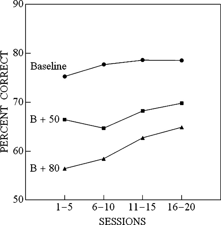
Figure 2 plots the mean percentage of stimuli correctly identified over the course of the experiment (in four blocks of five sessions) in each of the three conditions. This figure indicates that the addition of a fifth stimulus (50 or 80 dB SPL) resulted in a reduction in accuracy, with the reduction being more severe the more intense the added stimulus. There is also an indication that accuracy improves over time in each of the three conditions. A two-factor, within-participants ANOVA with condition (B, B + 50, and B + 80) as the first factor and block number as the second factor (blocks 1–4, referring, respectively to sessions 1–5, 6–10, 11–15, and 16–20) confirmed that there were significant main effects due to condition, F(2,10) = 32.495, p < .001, and block number, F(3,15) = 10.343, p < .001, as well as a significant condition × block interaction, F(6,30) = 2.47, p = .046. The interaction effect is due to the fact that while percent correct increased monotonically with session block for the B and B+80 conditions, performance in the first five sessions in B+50 was better than in the second five sessions. One-tailed t-tests indicated that accuracy, collapsed across blocks, was greater in the baseline than in the B + 50 condition, t(5) = 6.410, p < .001, which, in turn, was greater than that in the B + 80 condition, t(5) = 2.41, p = .030, as was expected.

Fig. 2.

Percent correct, averaged over participants, as a function of session block (five sessions to a block) in three conditions: (1) when the stimulus set in the absolute identification experiment contained four tones (baseline set = {25, 30, 35, and 40 dB SPL}); (2) when the stimuli consisted of the baseline set plus a 50-dB SPL tone (B + 50); and (3) when the stimuli consisted of the baseline set plus an 80-dB SPL tone (B + 80)

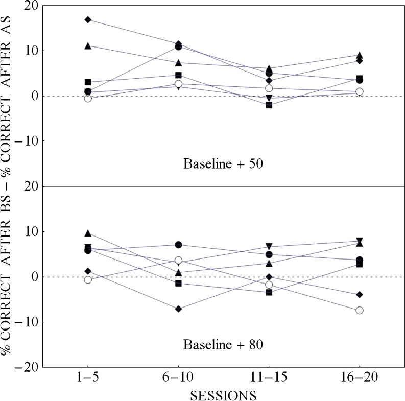
To examine whether the improvement seen in Fig. 2 was affected by where, in the trial sequence, the added loud stimulus appeared, we looked to see whether there was a difference in percent correct identification for the four baseline stimuli when they followed a baseline stimulus versus when they followed an added stimulus. Figure 3 plots, for each of the 6 participants, the difference between the percentage of times a baseline stimulus (25, 30, 35, 40 dB SPL) was correctly identified when it followed a baseline stimulus and the percentage of times a baseline stimulus was correctly identified when it immediately followed an added stimulus, as a function of block number. This figure suggests that this difference did not change over blocks of sessions in either the B + 50 or the B + 80 dB condition. This figure also suggests that in the B + 50 condition, but not in the B + 80 condition, participants, on average, performed better when a baseline stimulus followed another baseline stimulus than when it followed an added stimulus. A within-subjects ANOVA on the data from the B + 50 condition confirmed that the difference scores in this condition did not differ across blocks, F(3,15) = 2.04, p = .152, and that they were significantly different from 0, F(1,5) = 8.85, p = .031. The equivalent ANOVA on the data from the B+80 condition again failed to show a significant effect of trial block, F(3,15) = 1.46, p = .265, and could not reject the null hypothesis that the mean difference score was equal to 0, F(1,5) = 2.33, p = .187. Hence, the difference scores changed little over blocks, and only the difference scores for the B+50 condition differed significantly from zero.

Fig. 3.

The probability of a baseline stimulus being correctly identified given that it followed a baseline (BS) stimulus minus the probability of a baseline stimulus being correctly identified given that it followed an added stimulus (AS), as a function of session block when the added stimulus had a sound pressure level of 50 dB SPL (baseline + 50 condition) and when the added stimulus was 80 dB SPL (baseline + 80 condition). Data are presented for each individual in the experiment

A signal-detection analysis

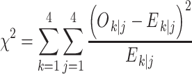
We also conducted a signal-detection analysis of these data. First we averaged the response-probability matrices across the 6 participants for each of the four session blocks to obtain four response-probability matrices for each condition. Two different models were evaluated. In the GEV model, we assumed that each stimulus gave rise to a normal (Gaussian) distribution of effects along a decision axis, with the observer locating three criteria (c ₁, c ₂, and c ₃) along this decision axis to produce four discrete response regions. In the LEV model, these normal distributions were replaced by equal-variance Laplace distributions. In each of these models,we searched for the parameter values that minimized the following quantity,

1

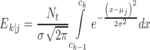
In this formula, O _k|j is the observed number of responses in response category k when stimulus j is presented; E _k|j, on the other hand, is the expected number of responses in category k when stimulus j is presented. If we define c ₀ = −∞, and c ₄ = ∞, and N _t as the number of trials per stimulus

2

in the GEV model, whereas

3

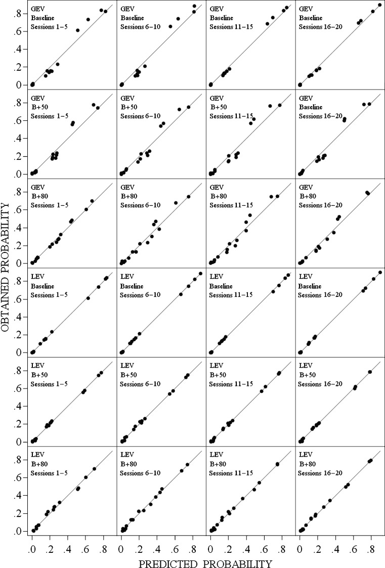
in the LEV model. Note that the quantity, χ ², in Eq. 1 is the Pearson chi-square statistic, a commonly employed measure of how well categorical data fit a model. In both models, the mean location of stimulus 1, μ ₁, was fixed at 0, and the standard deviation of each distribution, σ, was set to 1.0. A more detailed description of the fitting procedure is given in Parker et al. (2002). For each of the four session blocks in the three conditions, we found the parameter values for both the GEV and LEV models that minimized Eq. 1. These parameter values were then used to predict the probability of response k given stimulus j for all 16 combinations. The top four panels of Fig. 4 plot the obtained probabilities, O _k|j /N _t, against the probabilities predicted by the GEV model for the four session blocks in the baseline condition. The second and third rows of panels present the equivalent plots for the B+50 and B+80 conditions, respectively. If the fit were perfect in these panels, all points would fall on the positive diagonal. Note that the data points tend to depart systematically from the positive diagonal for the GEV model, falling below it for predicted probabilities < .4, and above it for predicted probabilities > .4.

Fig. 4.

The obtained probability of response k, (1 ≤ k ≤ 4), given stimulus j, (1 ≤ j ≤ 4), for the 16 combinations of k and j, as a function of the predicted values of these probabilities obtained from the best-fitting Gaussian equal-variance model and from the best-fitting Laplace equal-variance model for the baseline, B + 50, and B + 80 conditions. The models in each condition were fit to the matrices of stimulus–response probabilities averaged over participants and sessions. The straight lines represent where the points would fall in these coordinates if the predictions of the model were perfect

The bottom three panels present the equivalent plots for the LEV model. Note that in virtually every case, the LEV model provides a better fit to the data than does the GEV model. This was confirmed by a t-test comparing the 12 χ ² values obtained from the GEV model with those obtained from the LEV model, t(11) = 5.61, p < .001.

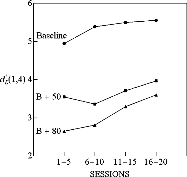
The gain-control model predicts a reduction of discriminability among the baseline stimuli when an additional stimulus is added to the baseline set, with the reduction in discriminability being greater when the intensity of the added stimulus is increased from 50 to 80 dB SPL. An estimate of the overall discriminability in the LEV signaldetection model can be obtained by determining the normalized distance between μ ₁ and μ ₄ in the fit to the LEV model. We refer to this as the Laplace d-prime range, which is defined as d′ _L(1,4) = (μ ₄ – μ ₁)/σ. Figure 5 plots the Laplace d-prime range as a function of the number of sessions in each of the conditions of the experiment. Note that the same pattern emerges as was found with percent correct in Fig. 2—namely, that d-prime range for the LEV model increases with the number of session blocks and is largest for the baseline condition, followed by the B+50 and B+80 conditions, respectively.

Fig. 5.

The distance along the decision axis between the stimuli 1 and 4 (25 and 40 dB SPL) scaled in Laplace d-prime units, as a function of session block for the baseline (B), B + 50, and B + 80 conditions. Each point is based on the Laplace equal-variance model that best fits the matrix of stimulus–response probabilities averaged over individuals for the session block in question

Individual performance

To determine the stability of individual differences in performance, we first examined the baseline condition to see whether the rank order of individuals with respect to overall percent correct differed over blocks of sessions. The reliability of individual differences was perfect over blocks. We measured this reliability with Kendall’s coefficient of concordance, W, and, in this case, W was, of course, equal to 1. In the B + 50 condition, it dropped to .96, and in the B+80 condition, it fell further to .83.

To compare how well the GEV and LEV models fit the data of individual participants, we constructed plots equivalent to Fig. 4 for each individual. An examination of these plots failed to provide any evidence that one model was reliably better than the other for any of the participants. Across all participants and conditions, the fit was better for the GEV than for the LEV model in 40 of the 72 instances—that is, in slightly more than half of the instances. In addition, no individual participant’s data were reliably better fit by one model than by the other.

Relative psychological distances among stimuli

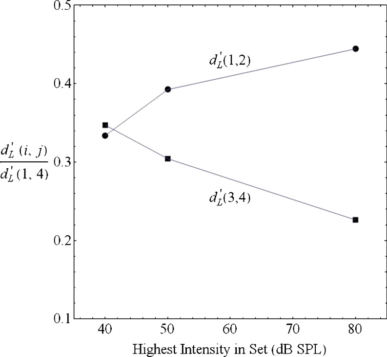
To examine whether the perceptual separation between adjacent stimuli changed as a function of the intensity of the loudest stimulus in the set, we first averaged the stimulus–response matrices separately for each participant across the 20 sessions. We then found the best-fitting Laplacian projection values along the decision axis for each participant. The Laplace d-prime between any two stimuli, i and j, is defined as the separation between their means along the decision axis, divided by their common standard deviation—that is, d′ _L(i, j) = (μ _j – μ _i)/σ. Figure 6 plots both d′ _L(1,2)/d′ _L(1,4) and d′ _L(3,4)/d′ _L(1,4) as a function of the highest intensity tone in the set. Figure 6 shows that the discriminability between the two lowest intensities in the set (25 and 30 dB SPL), relative to the discriminability of the softest and loudest baseline stimuli (d-prime range), increases with the intensity of the loudest stimulus, whereas the discriminability between the two highest intensities in the base set (35 and 40 dB SPL), relative to d-prime range, decreases as the intensity of the loudest stimulus in the set grows. All 6 participants exhibited the increasing pattern for the two lowest stimuli, and 4 of the 6 exhibited the decreasing pattern for the two highest stimuli in the base set. Figure 6 also shows that the two stimulus pairs were equally discriminable when there were only four stimuli in the set, but that the discriminability for the two softest tones exceeded that of the two loudest tones when there was a fifth tone in the set, and that relative difference grew as the intensity of the fifth stimulus increased.

Fig. 6.

The Laplace d-prime distance in a condition between stimuli 1 and 2 (circles), relative to the Laplace d-prime range between stimuli 1 and 4 in the same condition, is plotted as a function of the intensity of the highest tone in that condition. Also shown is the equivalent plot for the relative Laplace d-prime distance between stimuli 3 and 4 (squares)

Discussion

GEV versus LEV models

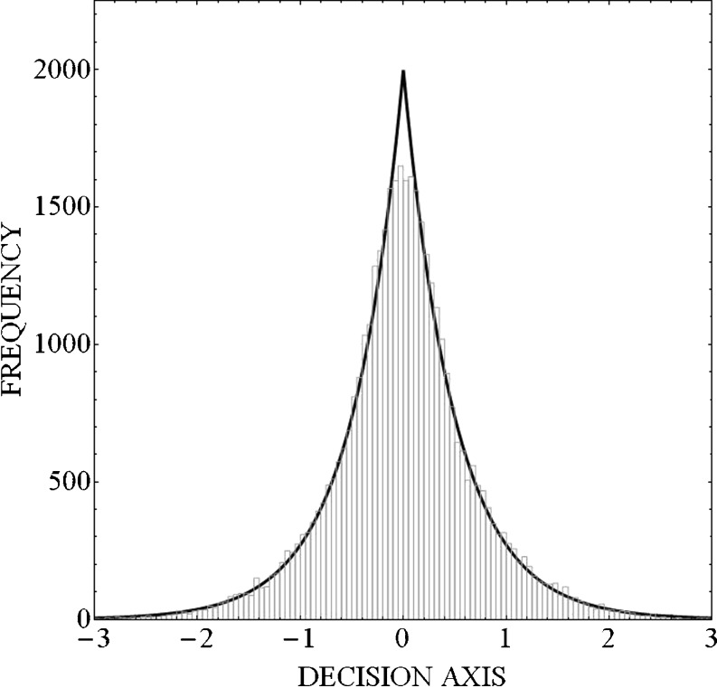
In signal-detection analyses of one-dimensional, m-alternative, AI experiments, it is usually assumed that the m stimuli give rise to m equal-variance Gaussian distributions along a unidimensional decision axis (see Macmillan & Creelman, 2005) . However, Parker et al. (2002), Gordon and Schneider (2007), and Murphy, Schneider, and Bailey (2010) have argued that equal-variance Laplace distributions provide a better fit to group AI data. This result is somewhat counterintuitive, especially if the distribution of effects along the decision axis are thought to arise from noise (or an accumulation of a large number of small errors) in the decision process, which, according to the central limit theorem, should give rise to Gaussian-shaped distributions. Schneider (2007) has shown that the Laplace distribution will provide a better description than the Gaussian distribution when responses to stimuli in an AI experiment are aggregated over participants with unequal sensory acuities, even when each individual participant’s data are equal-variance Gaussian. The LEV model would also fit better than the GEV model if data are aggregated over sessions within an individual if there are substantial changes in discriminability over time. To illustrate why this happens, in Fig. 7 we aggregated 10,000 random samples from each of four normal distributions having the same mean (μ = 0) but four different standard deviations (σ = 0.25, 0.50, 0.75, and 1.00, respectively) and plotted the histogram of the combined random samples (n = 40,000). Figure 7 shows that the Laplace distribution provides a very good fit to the aggregate of random samples from normal distributions having the same mean but different standard deviations. Hence, this is what we would expect the distribution of effects along the decision axis to look like if we aggregated responses to a stimulus across four individuals having different sensory acuities (different standard deviations) or within an individual when acuity is changing from session to session. Therefore, when discriminability is constant both across and within participants, we would expect the GEV model to provide the better fit if the decision process was based on equal-variance normal distributions. Because there is abundant evidence that discrimination performance differs across individuals (e.g., Nizami, Reimer, & Jesteadt, 2001), we should expect the LEV model to fit group data better than the GEV model.

Fig. 7.

Frequency histogram for the aggregation of 10,000 samples from each of four normal distributions having the same mean (μ = 0) but different standard deviations (σ = 0.25, 0.50, 0.75, and 1.0, respectively). The smooth curve fit to this histogram is what we would expect if the aggregate data were generated from a single Laplace distribution

The individuals in the present experiment differed substantially with respect to discrimination accuracy in the AI paradigm. Figure 2 also indicated that discrimination accuracy improved over time. To assess the degree of individual differences in discriminative sensitivity in this experiment, in each of the four blocks of sessions for each of the three conditions, we computed the ratio of the best performance achieved by one of the individuals in the block (in terms of percentage of correct identifications) with that of the worst performance achieved by one of the individuals in the same block. For instance, if the participant with the highest percentage of correct responses in block 2 in the B+50 condition correctly identified 75% of the stimuli, whereas the participant with the lowest percentage correct in the same block identified only 50% of the stimuli, the ratio of highest to lowest was 1.5. Because there were four blocks of trials for each of three conditions, 12 such ratios were computed. The geometric mean of those 12 ratios was 1.48, indicating a considerable range of individual differences within each block of trials for each of the three conditions. Hence, even if the AI decisions of each of the participants are based on the GEV model, we would nevertheless expect the LEV model to provide the better fit to the group data, as it indeed does in 11 of the 12 cases (see Fig. 4).

Within an individual, we would expect the LEV model to provide a better fit than the GEV model if there were substantial changes in performance over sessions, but the GEV to fit at least as well as the LEV model if there were only small changes over sessions. Within each condition, across the four blocks of trials within an individual, we determined the blocks with the highest and lowest average percentages of correct identifications. Because there were 6 participants in each of three different conditions, there were 18 such ratios indicating the maximum amount by which each individual differed across blocks. The geometric average of those 18 ratios (6 individuals × 3 conditions) was 1.1. In the 18 instances in which these ratios were computed, the GEV model provided the better fit in 10 of them. This is what we might expect if individuals’ decisions were often based on equal-variance normal distributions along the decision axis, with relatively little session-to-session variation. The fact that there was some variation in discriminability from block to block should have limited the proportion of cases in which the GEV model provided the better fit. A chi-square test indicated that the proportion of cases in which the GEV model provided the better fit was significantly higher when data were aggregated within individuals than when they were collapsed over individuals, χ ²(1) = 6.91, p < .01. Hence, it seems reasonable to conclude that the momentary performance of individuals is governed by the GEV model but that we can detect this only when there is stability across sessions. When there is not, or when data are aggregated across individuals who differ in discriminative sensitivity, the LEV model is to be preferred.

Why does the intensity of the fifth stimulus matter?

There are several theories that would predict that the addition of a high-intensity stimulus to a baseline set of low-intensity stimuli would reduce discriminability among the low-intensity tones. In Parker et al. (2002), we showed that the reduction in discriminability was not a simple effect of stimulus range, as described in the theories of Durlach and Braida (1969) and Gravetter and Lockhead (1973). According to range theories, discriminability among a set of stimuli should decrease as the range between the highest and lowest intensities in the stimulus set increases. In Parker et al., discriminability among the four tones in the low-intensity baseline set (25, 30, 35, and 40 dB SPL) did decrease as the intensity of the fifth added tone and, therefore, stimulus range increased. However, when the baseline set consisted of four high-intensity tones (84.5, 86.5, 88.5, and 90.5 dB SPL) and a fifth lower intensity tone was added to the baseline set, discriminability among the four baseline tones remained essentially unchanged as the intensity of the fifth tone was lowered from 80.5 to 40 dB SPL (i.e., the range increased; see their Fig. 4). This asymmetrical response to increases in range cannot be easily accounted for in range effect models. However, there still remain several other possible explanations for the effects observed here.

One is the idea that the reduction in discriminability is due to passive adaptation-like effects in which exposure to loud sounds depresses responsiveness to subsequent sounds. Adaptation theories might predict that a sensory response to a stimulus that immediately followed a high-intensity adapting stimulus would be reduced, relative to the response that would occur otherwise. This would predict that discriminability and identification would be worse when the added tone was 80 dB SPL than when it was only 50 dB SPL, which indeed did occur. However we would also expect that the probability of correctly identifying a baseline tone would be lower for a tone following an 80-dB SPL tone than for one following another baseline tone. Figure 3, however, indicates that the probability of correctly identifying a tone from the baseline set is little affected by whether or not it is preceded by an 80-dB SPL tone. Adaptation-based accounts would expect this to occur only if recovery from adaptation to a high-intensity tone was complete by the time the succeeding tone was presented, or if recovery from adaptation was so slow that the occasional 80-dB tones kept the participants’ sensitivity fully depressed throughout the experiment. (See Arieh, Kelly, & Marks, 2005, for some evidence that the latter condition might be met for induced loudness reduction, a phenomenon that Arieh and Marks 2011, regard as adaptation-like.) However, neither of these appeared to occur in Experiment 4 in Parker et al. (2002). In that study’s low-intensity condition, participants discriminated (in a 2IFC procedure) between two relatively soft 1-kHz tones (in the range from 25 to 30 dB SPL) with an average accuracy of about 83%. When, on one-third of the trials, the louder of those two tones was unpredictably replaced by a 92-dB SPL 1-kHz tone, accuracy dropped to about 70% on the remaining two-thirds of the trials that involved only the original soft tones. This is incompatible with an adaptation process with very fast recovery. However, when all trials asked participants to discriminate the two baseline soft tones but included a 92-dB SPL 1-kHz “warning tone,” performance fell only to about 79% and did not differ significantly from baseline. This is incompatible with an adaptation process with very slow recovery times. Thus, adaptation is not a reasonable explanation for the results reported in that study.

Another possible explanation lies in attention-allocation effects (Luce & Green, 1978; Nosofsky, 1983; Nosofsky & Luce, 1984), that there is an attention band of limited range (approximately 10 dB; Luce & Green, 1978) that the participant directs to particular regions of the intensity range. Such theories of attention allocation cannot readily account for the reduced discriminability observed with the addition of a remote high-intensity stimulus. Consider first theories of attention allocation in which participants are completely free to allocate their attentional resources to different intensity regions. For the baseline set of stimuli, the average relative discriminability (d′ _L) between adjacent stimuli was .33 between 25- and 30-dB SPL stimuli, .32 between the 30- and 35-dB SPL stimuli, and .35 between the 35- and 40-dB stimuli. From an attentional allocation point of view, this would indicate that attentional resources were spread evenly across the range from 25 to 40 dB SPL. Now if attention allocation were purely a top-down phenomenon and if listeners were free to allocate attention to whatever intensity ranges were optimal, they need not change their attentional focus when the 80-dB SPL tone was added to the baseline set, since there should be no problem in identifying the 80-dB SPL tone, regardless of where along the intensity dimension their attentional resources were focused. Hence, identification performance for the four lowest intensity stimuli should have remained the same when the 80-dB SPL tone was added to the baseline set. Because discriminability was reduced when the high-intensity tone was added, we must assume, within an attention-allocation framework, that attentional resources were reallocated as a result of the introduction of the high-intensity tone.

Some theories of attention (e.g., Luce, Nosofsky, Green, & Smith, 1982) hypothesize that the attention band is involuntarily drawn to the intensity region of the most recently presented stimulus and/or to the anchor stimuli (the highest and lowest intensities in the stimulus set). A shifting attention band would predict better performance when a stimulus is preceded by a stimulus with a similar intensity than when it follows a stimulus whose intensity is quite remote. Clearly, a baseline stimulus that follows an 80-dB SPL anchor stimulus is remote from its predecessor and, according to such a theory, should be harder to identify than when it follows one of the stimuli in the baseline set (25, 30, 35, 40 dB SPL) if the attention band tends to track the previous stimulus. However, identification accuracy for a baseline stimulus in the B+80 condition was the same independently of whether it was preceded by another baseline stimulus or by an 80-dB SPL stimulus (see Fig. 3). This result suggests that the location of the attention band remains fixed throughout the session, which would defeat the utility of an attention band explanation of AI data. For these reasons, theories of attention allocation cannot readily account for the AI data from this study. (The most recent version of the theory [Nosofsky & Luce, 1984] held that the location of the attention band is drawn “in a somewhat sluggish fashion to region ‘where the action is’” [p.24] rather than on a trial-by-trial basis to the location of the previous stimulus. No definite predictions about the present data emerge clearly from this model.)

A nonlinear gain-control model under top-down control

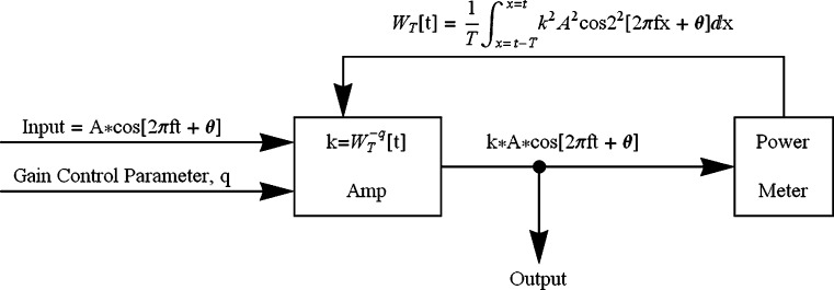
Parker and Schneider (1994) developed a nonlinear gain-control model that could account for many of the properties of nonmetric comparisons of loudness differences. In a skeletal version of the model, an auditory signal is passed through a bank of band-pass filters before being sent to an amplifier under feedback control. Figure 8 indicates how this model would work when the input to the amplifier is a sine wave. Basically, the momentary gain of the amplifier is specified as k, so that the momentary output of the amplifier is simply k times the input, which, in this example, is a sine wave. The output, however, goes to a power meter that determines the average power, W _T, in the signal over time period T. A feedback loop then determines the gain for the next T-second period on the basis of the average power of the preceding T-second period, where the gain, k, is equal to W ^-q, where q is under top-down control. In the present experiment, it is assumed that the listener has an expectation as to the loudest stimuli that are likely to occur in a session and adjusts q to protect against a sensory overload and to maximize discriminability. Specifically, as anticipated maximum intensity grows, so does q. Note that the consequence of increasing q is to increase compression (lower the value of k) in the model. Parker and Schneider (1994) showed that, when the input is a steady-state signal, this circuit converges rapidly to a steady-state output when the value of q is in the range of 0.1–0.3. In particular, when the input is a steady-state sinusoid [A Cos(2 π f _c t + θ)], the steady-state output is

4

Fig. 8.

An amplifier with a negative feedback loop. Power at the output of the signal is used to modulate the gain on the amplifier. As the power at the output increases, the amplifier’s gain is reduced. The amount of compression is governed by the value of q, which is assumed to be under top-down control (see the text)

Hence, this circuit predicts that the response of the auditory system to a pure tone is a power function of sound pressure whose exponent varies with the amount of compression (the greater the compression, the lower the exponent).

In addition to top-down control over the amplifier’s gain, we also assume that there is top-down control over a threshold sensor such that a signal enters this gain-control system only if it exceeds a specific root-mean square (RMS) sound pressure level. Specifically, subthreshold signals have no consequence. It is important to note that the threshold value for this sensor need not be the sensory system’s absolute threshold but is, instead, a second parameter that can be influenced by a listener’s expectations. Effectively, what this threshold sensor does is increase discriminability for stimuli near the lowest expected intensity in the stimulus set by enhancing the growth of loudness in this region.

In the model, the observer’s settings of the gain on the amplifier will determine the location of the mean value,μ _j, of the distribution of effects along the decision axis arising from repeated presentations of stimulus j, without changing the variance, σ, of these distributions.2 Hence, changing the amplifier’s gain will nonlinearly alter the positions of the distributions shown in Fig. 1, but not their variances. In modeling both group and individual data, we have chosen to use the Laplace distribution throughout, because the available evidence suggests that individuals vary in sensitivity and that sensory acuity improves with experience (see Figs. 2 and 5). Hence, we would expect the Laplace distribution to better characterize the hypothetical distribution of effects along the decision axis.

Another assumption in the model is that the variance depends on the number of criteria needed to define the response regions. Because the baseline set contains four stimuli (three criteria), while the sets with the added stimulus contain five stimuli (four criteria), in fitting the model, we needed to fit two estimates of variance, one for the baseline set and the other for any set containing five stimuli. However, in fitting the model, we found that a ratio of variance, r _v, in the four-stimulus case to that in the five-stimulus case of .71 provided a good fit to all of the data sets, effectively reducing the variance estimate to a single parameter.

The fleshed-out model (see the Appendix) has six free parameters, c, p _T, n, s, σ ₃, and r _v, where σ ₃ is the standard deviation of the Laplace distribution when three criteria are needed, r _v is the ratio of σ ₃ /σ ₄, c is a dimensional constant translating sound pressure into neural activity, n is the highest value that q can reach, s is a parameter determining how fast that value is approached as the expected maximum intensity increases, and dB_T is the sound pressure level that must be exceeded before the gain-control circuit is activated. To find the best-fitting values of the model’s parameters, we computed the Laplace d-prime distances between all pairs of stimuli in a particular condition. Because there were four stimuli in the baseline stimulus set, there were six pairwise Laplace d-primes per condition. These d-prime values were taken from the signal-detection analysis. Thirty-four conditions in all were examined: the eight low-intensity conditions from Parker et al. (2002), the eight high-intensity conditions from Parker et al., and the three conditions for each of the 6 individual participants in the present experiment. To solve for the best-fitting parameter values, we systematically varied p _T and, simultaneously, found the parameter values that produced the minimum sum of squared errors between the obtained d-prime values and those predicted from the program, using Mathematica’sNonlinearRegression algorithm. The values of the model’s parameters are given in Table 1. The Appendix provides a more detailed description of the model.

Table 1.

Values of n and σ ₃ for the group of participants from Parker et al. (2002), and for the 6 participants from the present experiment for the gain-control model. The value of n did not vary across stimulus sets. The values of σ ₃ in this table specify the standard deviation of the Laplace distributions when the stimulus set contained only four elements (three criteria). For stimulus sets containing five elements (four criteria), the value of the standard deviation of the Laplace distributions, σ ₄, was found to be 1.19 σ ₃. The value of dB_c in this model was 20.05, the value of s was 25.22, and the value of dB_T was 24.3

Experiment or Participant	Stimulus sets (Elements of the set are the intensity values of the tones in dB SPL)	n	σ 3
Parker et al. (2002)	{25, 30, 35, 40}, {25, 30, 35, 40, 45},	0.27	0.597
	{25, 30, 35, 40, 50}, {25, 30, 35, 40, 55},
	{25, 30, 35, 40, 60}, {25, 30, 35, 40, 70},
	{25, 30, 35, 40, 80}, {25, 30, 35, 40, 90},
	{84.5, 86.5, 88.5, 90.5}, {40, 84.5, 86.5, 88.5, 90.5},
	{50.5, 84.5, 86.5, 88.5, 90.5}, {60.5, 84.5, 86.5, 88.5, 90.5},
	{70.5, 84.5, 86.5, 88.5, 90.5}, {75.5, 84.5, 86.5, 88.5, 90.5},
	{80.5, 84.5, 86.5, 88.5, 90.5}, {82.5, 84.5, 86.5, 88.5, 90.5}
P1	{25, 30, 35, 40}, {25, 30, 35, 40, 50}, {25, 30, 35, 40, 80}	0.2	0.983
P2	{25, 30, 35, 40}, {25, 30, 35, 40, 50}, {25, 30, 35, 40, 80}	0.36	0.619
P3	{25, 30, 35, 40}, {25, 30, 35, 40, 50}, {25, 30, 35, 40, 80}	0.22	0.649
P4	{25, 30, 35, 40}, {25, 30, 35, 40, 50}, {25, 30, 35, 40, 80}	0.12	0.78
P5	{25, 30, 35, 40}, {25, 30, 35, 40, 50}, {25, 30, 35, 40, 80}	0.27	0.598
P6	{25, 30, 35, 40}, {25, 30, 35, 40, 50}, {25, 30, 35, 40, 80}	0.38	0.223

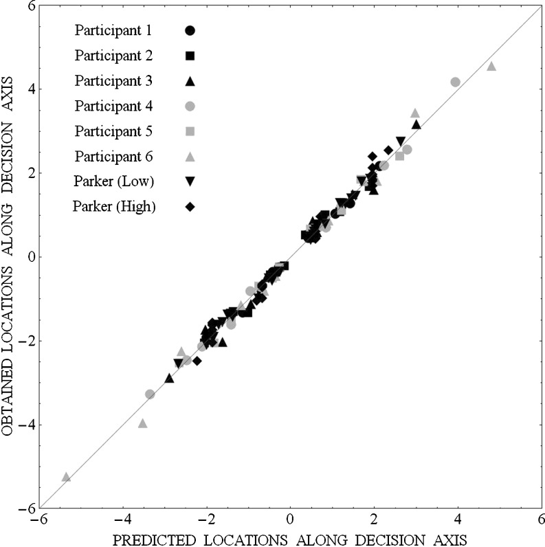
The predicted d-prime values were used to determine the mean locations of the stimuli (hereafter called their projection values) along the decision axis in each of the 34 conditions in the following way. First, the projection value of the lowest stimulus in the base set was fixed at zero. Second, the projection value of the second stimulus in the set was set to the value of the predicted d-prime between stimulus 1 and stimulus 2, and so on for all stimuli. Then the mean of the predicted projection values along the decision axis was subtracted from each projection value, so that the resulting predicted projection values had a mean of zero in each condition. The mean of the obtained projection values in a condition was also subtracted from each of the obtained projection values in that condition, so that the average of the obtained projection values also had a mean of zero. Figure 9 plots the obtained projection values as a function of the projection values predicted by the model. The straight line represents perfect agreement between obtained and predicted projection values. Because the deviations from this straight line are minimal, we conclude that the model provides an excellent fit to the data. It should be noted that single values of c, p _T, and s were used for all conditions. Hence, the only parameters that distinguished one participant from another or from the group of participants in Parker et al. (2002) were σ ₃, the variance when there are three criteria, and n, the asymptotic value of the feedback parameter, q. Note that the s parameter specifies how fast the asymptotic value of q is approached as the expected maximum intensity increases.

Fig. 9.

Projection values along the decision axis obtained from the Laplace equal-variance model as a function of the projection values predicted by the gain-control model for the data of the 6 participants in the three conditions of the present experiment and the data of the groups of participants in the low- and high-intensity baseline conditions in Parker et al. (2002)

A significant advantage of the model is that it predicts that as the intensity of an added stimulus is increased, not only will discriminability among a set of low-intensity stimuli decrease, but in addition discriminability among the highest intensities in the baseline set, relative to the discriminability of stimuli 1 and 4, will decline more rapidly than will the corresponding discriminability among the lower intensities (see Fig. 6), something that adaptation theories and attention-allocation theories cannot easily accommodate. It also accounts for the fact that the addition of a low-intensity stimulus to a set of four high-intensity stimuli has a far smaller effect than the reverse (Parker et al., 2002), something that theories based on stimulus range have difficulty in accommodating.

A second advantage of the model is its correspondence to measurement of compression in the mechanical input/output (displacement) functions of the basilar membrane in cat, chinchilla, gerbil, and guinea pig. For all of those, the input/output functions are linear up to about 20–25 dB SPL and compressive for higher input levels (see Cooper, 2004, for a thorough review). Thus, it is interesting that in fitting the model to data (see the Appendix), p _T in dB SPL proved to have a value of 24.3 dB, precisely where compression begins to occur in the cochlea. Unfortunately, none of the studies used to fit data to the model included any stimuli with intensities below 25 dB SPL (i.e., in the linear range in the cochlea), and so we cannot be certain that p _T would be unchanged were such data to be included. Nonetheless, the correspondence of the model to this physiological data is encouraging.

Finally, a critical feature of the model is that it is under top-down control. Applications of the model with respect to auditory intensity (Gordon & Schneider, 2007; Parker et al., 2002) and visual contrast (de la Rosa et al., 2009; Mišić et al., 2010) indicate that compression is applied only when the observer expects high-intensity stimuli but cannot predict when they will occur. We have previously discussed the results of Experiment 4 of Parker et al. and their incompatibility with an adaptation-based account of the outcome of the present study. In studies of visual contrast, both de la Rosa et al. and Mišić et al. compared absolute identification of contrast gratings in a baseline condition in which only low-contrast sine wave gratings were presented against performance in two other conditions: (1) a condition in which a high-contrast grating was randomly added in an unpredictable fashion to the baseline set of low-contrast gratings (baseline + unpredictable high-contrast stimulus) and (2) a condition in which different fixation symbols reliably predicted the occurrences of high- and low-contrast gratings (baseline + predictable high-contrast stimuli). In both those experiments, the addition of an unpredictable high-contrast stimulus reduced discriminative performance among the low-contrast baseline stimuli, whereas the addition of a predictable high-contrast stimulus did not. This indicates that the observer can rapidly adjust the gain in visual contrast on the basis of momentary expectations concerning the intensities of stimuli that are likely to occur, much as appears to occur in loudness.

The linkage between sensation and discriminability

The relationship between sensory experience (e.g., loudness) and discriminability has been a contentious one ever since Fechner’s (1966) pioneering attempt to link sensation to intensity via the argument that “equally-often noticed differences are subjectively equal.” The fact that judgments of loudness are affected by context raises the issue of whether the effects of context on loudness are mediated, in part, by a nonlinear gain-control mechanism. If we assume that the loudness (perceived intensity) of a sound is directly proportional to the output of the nonlinear gain-control mechanism proposed here, then

5

where a is a scalar constant linking loudness judgments to the mean positions of the distributions of effects along the decision axis, and q is determined according to Eq. A4 in the Appendix. Note that this form of the loudness function corresponds to Scharf and Stevens’s (1961) threshold adjustment to the Stevens power law. Hence, it accounts for the more rapid growth in loudness with intensity near the listener’s threshold. The major difference between this model and that of Scharf and Stevens is that, in the gain-control model, the threshold parameter and the value of the exponent of the power function are assumed to be under top-down control, with the exponent being reduced as the maximum expected intensity increases. It is also interesting to note that when high-intensity stimuli are present (> 90 dB SPL), the exponent of the power function in Eq. 5 (using the parameters fit to the data of Parker et al., 2002), is approximately 0.29 as a function of sound pressure, a value that is quite close to the value found for nonmetric scaling of loudness differences (Parker & Schneider, 1974; Schneider, Parker, & Stein, 1974; Schneider, Parker, Valenti, Farrell, & Kanow, 1978).

The present model also illustrates one of the difficulties involved in linking sensory magnitude to discriminability. Assume that sensory magnitude is governed by Eq. 5 in loudness estimation experiments, and that Eq. 5 also determines the mean position of each stimulus along the decision axis in AI experiments. Because participants 2 and 6 (see Table 1, P2 and P6) have identical values of c, p _T, and dB_max and nearly equivalent values of n (.36 and .38, respectively), their loudness functions will be nearly identical according to Eq. 5. Discriminability among a set of stimuli will, nonetheless, differ between them because, although the locations of the means of the distributions of effects along the decision axis are the same for both of them, the standard deviation of the distributions for participant 2 is almost three times as large as the standard deviation for participant 6. Hence, even though they have the same loudness function, participant 6 will outperform participant 2 in an AI experiment.

Conclusions

These studies, taken together, support the hypothesis that sensory intensity is modulated by a nonlinear amplification system in which the gain is directly controlled by the observers’ expectations concerning the stimulus intensities they are likely to experience. This system serves to protect the individual from sensory overload. Moreover, the ability to rapidly reset the gain permits the observer to maximize discriminability within a particular intensity range while simultaneously providing protection from damage due to sensory overload.

Appendix: The Model

The present model is a generalization of the one presented in Parker and Schneider (1994). Let x(t) be the input to the linear auditory filter (see Fig. 10). The output of the filter is c*H[x(t)], where H[x(t)] is the linearly filtered version of the signal and c is a dimensional constant that converts sound pressure into its neural equivalent at the output of the filter. If the filter is sufficiently narrow, we can express the output of the filter over a period of T seconds (T = 1/f _c) as being essentially equivalent to

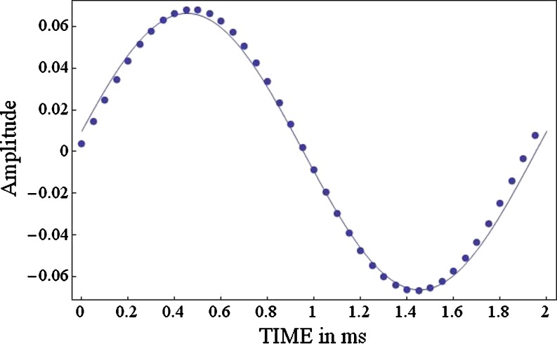
and θ _x is the phase of the sine wave that best matches that of H[x(t)] over the T-second period. Figure 11 shows 2 ms of the digitized output of an auditory filter (gamma-tone filter, center frequency = 500 Hz, equivalent rectangular bandwidth = 96 Hz) to a band-limited white noise (bandwidth = 10 kHz, sampling rate = 20 kHz). Figure 11 shows that an arbitrary output can be well matched to a 500-Hz pure tone whose amplitude is and whose phase is θ _x.

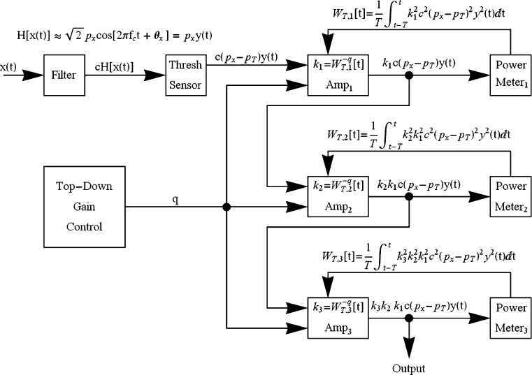
Fig. 10.

The full nonlinear gain-control circuit, after translating the output of the linear filter to its neural equivalent, routes the output to a threshold sensor that passes only the amount of energy in the signal that exceeds some threshold value. The output from the sensor then passes through three concatenated nonlinear amplifiers of the type shown in Fig. 8 to allow for a greater range of compression and more rapid convergence to a steady-state output when the input is a steady-state signal. The amount of feedback is controlled by the parameter q, which is assumed to be under top-down control

Fig. 11.

The points specify the digitized output from a narrowband filter (gamma-tone, center frequency = 500 Hz, equivalent rectangular bandwidth = 96 Hz) to a band-limited Gaussian noise (bandlimit = 10 kHz) over a period of 2 ms. The smooth curve fit to these points is the best-fitting sine wave over this period

In the model there is a sensor that serves to trigger the gain-control circuitry. This sensor responds only when the RMS sound pressure in the filtered stimulus exceeds a certain minimum trigger value, p _T. Effectively, then, the level of the signal that serves as input to the gain-control portion of the circuit is the amount by which the filter’s output exceeds the trigger value. Hence, the output of the sensor, over the time period T, is approximately

A1

where p _T is the RMS sound pressure level in dB of a steady-state pure tone of frequency, f _c, that just reaches the sensor’s threshold, and θ _x represents the phase of the pure tone that best matches the phase of the filtered signal at that point of time. The output of the sensor, in turn, serves as the input to three concatenated gain-control units of the type shown in Fig. 10, with each of the units under the top-down gain-control parameter q. Three units were chosen to keep the value of q within the range of quick convergence to a steady state input.

Let f _c be the center frequency of the filter. Now consider a pure tone whose frequency is f _c and whose RMS sound pressure is p _x. It can be shown that the steady-state output of the gain-control circuit to this pure tone is

A2

To avoid having to specify c, p _x, and p _T in sound pressure units, we now define,

where p ₀ is the reference SPL, and express the output of the circuitry shown in Fig. 10 in terms of the dB equivalents of c, p _x, and p _T. When these quantities are expressed in decibels, the output of this circuit to a sinsusoidal input whose RMS amplitude is p _x is

A3

Note that the model has three parameters, c, p _T, and q. The assumption in this model is that q, the compression factor, is selected on the basis of the highest anticipated intensity that might occur on a trial. To fit the model to the data, we assumed that q varies in an exponential fashion with the dB value of the maximum intensity produced at the output of the filter by any stimulus in the set. Hence, q was assumed to be an exponential function of 20 Log₁₀(p _Max* c) = dB_Max-dB_c , where p _Max is the maximum RMS sound pressure at the output of the linear filter. Hence q varies according to the function

A4

When the maximum intensity stimulus is a pure tone whose center frequency is f _c, dB_Max is the dB SPL value of that pure tone, n is the asymptotic value of q, and s is a parameter that determines how quickly q approaches that asymptotic value. Hence, the mean location along the decision axis of a pure tone stimulus at the center frequency of the filter, whose sound pressure level is dB_x, is

A5

where the value of q is specified by Eq. A4.

Note that, in this model, the compression parameter, q, is based on the maximum RMS amplitude experienced at the output of the filter when the listener cannot predict its occurrence and that there are two parameters: n, the maximum value of q, and s, the parameter that determines the rate at which q approaches n as the maximum sound intensity increases. Hence, the gain-control model mapping sound intensity onto the decision axis has four parameters:c, p _T, n, and s.

In applying the model, we assumed that the distribution of stimulus effects along the decision axis varies according to a Laplace distribution. Specifically, we assumed that the distribution of effects, x, along the decision axis for a monaural stimulus whose sound pressure level is dB_x and where the loudest tone presented in the session is dB_Max has the density function

A6

where σ is the standard deviation of the Laplace distribution. The locations of these stimuli, scaled in Laplace d-prime units, can then be obtained by dividing μ[dB_x] by σ. Hence, the Laplace d-prime between any two stimuli j and k (dB_j>dB_k) is given by μ[dB_j]/σ-μ[dB_k]/σ.

To solve for the best-fitting parameter values, we systematically varied dB_T and, simultaneously, solved for the parameter values that produced the minimum sum of squared errors between the obtained d-prime values and those predicted from the program, using Mathematica’sNonlinearRegression algorithm, subject to the restriction that dB_c, dB_T, and s were invariant across conditions and experiments. The best-fitting values of dB_c, dB_T, and s were 20.05, 24.3, and 25.22, respectively. The values of n and σ ₃, which were constrained to be the same for the 16 conditions tested in Parker et al. (2002) and for any individual participant in the present experiment, are given in Table 1. The values of σ ₃ in this table specify the standard deviation of the Laplace distributions when the stimulus set contained only four elements (three criteria). For stimulus sets containing five elements (four criteria), the value of the standard deviation of the Laplace distributions, σ ₄, was found to be equal to 1.195 σ ₃.

To assess the degree to which this fitting routine could distinguish a condition in which the amplifier’s gain was controlled by the highest expected intensity in the data set from one in which there was no gain control, we simulated data sets with and without gain control. In simulating sets of data without gain control, we assumed that the mean position of a stimulus along the decision axis was given by

A7

Note that, in this model, it is assumed that loudness is a power function of sound pressure with an exponent equal to 1/(1 + 2n _A)³, and that a constant, c, expressed in dB (dB_c), translates this power function into a point along the decision axis. Note also that this equation differs from Eq. A5 in two respects. First, the exponent is assumed to be independent of the loudest sound in the set. Second, there is no threshold parameter, p _T, that specifies the intensity level at which gain control kicks in, because there is no gain control in this model. All other aspects of the model were assumed to be the same as those in the full gain-control model. In total, we simulated 100 independent data sets corresponding to the 34 stimulus conditions indicated in Table 1. In these simulations, we set c = 1 so that dB_c = 0, and, using Eq. A7, generated eight sets of hypothetical positions along the decision axis for the baseline stimuli used in the present experiment, setting the value of n _A to the corresponding value of n in Table 1. Specifically n _A was set to 0.27 for the two baseline sets ({25, 30, 35, 40 dB SPL} and {82.5, 84.5, 86.5, 88.5 dB SPL}) in Parker et al. (2002) and to 0.20, 0.36, 0.22, 0.12, 0.27, and 0.28 for participants P1 to P6, respectively, for the baseline conditions {25, 30, 35, 40 dB SPL} in the present experiment. In the simulation, the standard deviation of the Laplace distributions was set to 0.6 for all baseline conditions (which corresponded to an expected value of 71% correct identifications for participant P1, assuming that this participant’s criteria were set midway between the mean stimulus positions along the decision axis). When an additional stimulus was added to the set, the value of the standard deviation of each of the Laplace distributions was increased to 1.195 * 0.6. To generate a stimulus–response probability matrix, it was assumed that the decision criteria were midway between the projection values. Eq. 2 was then used to generate each of the 16 entries in the stimulus–response probability matrix. Once the four probabilities were determined for each stimulus, Mathematica’s Multinomial Random number generator was used to generate the number of times out of N trials that stimulus j was classified as stimulus 1, 2, 3, or 4. The number of trials was set to 500 for the conditions tested in Parker et al. and to 1,000 for the conditions tested in this experiment. This probability matrix then served as input to a second program used to find the “obtained” projection values for this simulated experiment. This procedure was repeated 100 times for each of the 34 conditions illustrated in Table 1.

The mean and standard deviations of the obtained values of n of the gain-control model fit to the simulation of data without gain-control, along with the values of n used to generate these simulations, are shown in Table 2. This table indicates that the gain-control model can accurately capture the asymptotic values of the exponents of the power function when the model does not include gain control. The mean value (1.189) of the ratio of σ ₄/σ ₃ did not differ significantly from that (1.195) used to generate the simulations, t(99) = −1.60, p > .1.

Table 2.

Mean values and standard deviations (in parentheses) of n obtained (n obt) from 100 simulations of absolute identification experiments in which the mean locations of the stimuli along the decision axis were determined in the absence of gain control. Also shown are the hypothetical values of n used in the generation of these simulations (n start). For stimulus sets containing five elements (four criteria), the average value of the standard deviation of the Laplace distributions, σ ₄, was found to be 1.189 σ ₃. The average values of dB_c, dB_n, and s in this model were 7.79, –46, and 4.99, respectively

Experiment or Participant	Stimulus sets (Elements of the set are the intensity values of the tones in dB SPL)	n obt	n start
Parker et al. (2002)	{25, 30, 35, 40}, {25, 30, 35, 40, 45},	0.27 (.01)	0.27
	{25, 30, 35, 40, 50}, {25, 30, 35, 40, 55},
	{25, 30, 35, 40, 60}, {25, 30, 35, 40, 70},
	{25, 30, 35, 40, 80}, {25, 30, 35, 40, 90},
	{84.5, 86.5, 88.5, 90.5}, {40, 84.5, 86.5, 88.5, 90.5},
	{50.5, 84.5, 86.5, 88.5, 90.5}, {60.5, 84.5, 86.5, 88.5, 90.5}, {70.5, 84.5, 86.5, 88.5, 90.5}, {75.5, 84.5, 86.5, 88.5, 90.5}, {80.5, 84.5, 86.5, 88.5, 90.5}, {82.5, 84.5, 86.5, 88.5, 90.5}
P1	{25, 30, 35, 40}, {25, 30, 35, 40, 50}, {25, 30, 35, 40, 80}	0.20 (.02)	0.20
P2	{25, 30, 35, 40}, {25, 30, 35, 40, 50}, {25, 30, 35, 40, 80}	0.38 (.15)	0.36
P3	{25, 30, 35, 40}, {25, 30, 35, 40, 50}, {25, 30, 35, 40, 80}	0.21 (.03)	0.22
P4	{25, 30, 35, 40}, {25, 30, 35, 40, 50}, {25, 30, 35, 40, 80}	0.12 (.02)	0.12
P5	{25, 30, 35, 40}, {25, 30, 35, 40, 50}, {25, 30, 35, 40, 80}	0.27 (.06)	0.27
P6	{25, 30, 35, 40}, {25, 30, 35, 40, 50}, {25, 30, 35, 40, 80}	0.45 (.23)	0.38

To see whether the model accurately reflects the lack of gain control in these simulations, the obtained values of dB_c and s were used to plot the function describing how closely q (expressed as a percentage) approached its asymptotic value as the maximum intensity in the stimulus set increased. Specifically, the percentage of the asymptotic value of q is given by

A8

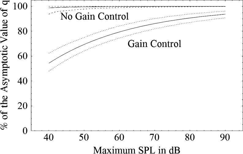
One hundred such functions were generated for the 100 simulations and were used to determine the average function describing how closely q approached its asymptotic value (upper solid line in Fig. 12), as well as to estimate the 95% confidence interval for this function (dotted lines bracketing the upper solid line). Figure 12 indicates that when the simulations did not involve gain control, the parameters of the gain-control function fit to such data reflect the absence of gain-control by indicating that gain does not change substantially with the maximum intensity in the stimulus set.

Fig. 12.

The mean percentage of the asymptotic value of the gain-control parameter q as a function of the maximum stimulus intensity for sets of simulations that did not include gain control (upper solid line) and those that did (lower solid line). Also shown are the 95% confidence limits for these mean functions

We also checked the accuracy of the fitting procedure by simulating 100 sets of data with gain control. In these simulations, the values of the parameters of the gain-control model found to fit the data in the article (see Table 1) were used to generate projections along the decision axis. These projection values were used to generate stimulus–response probability matrices as described above for the simulations that did not include gain. The value of σ ₃ in these simulations was set to 1.40, since that produced an average percent correct = 71% for participant 1 in the baseline stimulus set. Hence, the standard deviation along the decision axis was adjusted so that the gain-control simulations produced the same percentage correct for P1 in the baseline condition.

The parameter values found for these simulations are shown in Table 3. Table 3 indicates that when the simulations modeled a system with gain control, the fitting procedure accurately captured the parameters of the model. The degree to which q increased with the maximum intensity in the stimulus set is also shown in Fig. 12, along with its 95% confidence limits. Thus, Fig. 12 shows that the fitting procedure used here can accurately and clearly discriminate between the presence and absence of gain control.

Table 3.

Mean values and standard deviations (in parentheses) of n obtained (n obt) from 100 simulations of absolute identification experiments in which the mean locations of the stimuli along the decision axis were determined in the presence of gain control. Also shown are the hypothetical values of n used in the generation of these simulations (n start). For stimulus sets containing five elements (four criteria), the average value of the standard deviation of the Laplace distributions, σ ₄, was found to be 1.194 σ ₃. The average values of dB_c, dB_n, and s in this model were 19.94, 24.31, and 25.32, respectively

Experiment or Participant	Stimulus Sets (Elements of the set are the intensity values of the tones in dB SPL)	n obt	n start
Parker et al. (2002)	{25, 30, 35, 40}, {25, 30, 35, 40, 45},	0.27 (.003)	0.27
	{25, 30, 35, 40, 50}, {25, 30, 35, 40, 55},
	{25, 30, 35, 40, 60}, {25, 30, 35, 40, 70},
	{25, 30, 35, 40, 80}, {25, 30, 35, 40, 90},
	{84.5, 86.5, 88.5, 90.5}, {40, 84.5, 86.5, 88.5, 90.5},
	{50.5, 84.5, 86.5, 88.5, 90.5}, {60.5, 84.5, 86.5, 88.5, 90.5}, {70.5, 84.5, 86.5, 88.5, 90.5}, {75.5, 84.5, 86.5, 88.5, 90.5}, {80.5, 84.5, 86.5, 88.5, 90.5}, {82.5, 84.5, 86.5, 88.5, 90.5}
P1	{25, 30, 35, 40}, {25, 30, 35, 40, 50}, {25, 30, 35, 40, 80}	0.20 (.02)	0.20
P2	{25, 30, 35, 40}, {25, 30, 35, 40, 50}, {25, 30, 35, 40, 80}	0.36 (.03)	0.36
P3	{25, 30, 35, 40}, {25, 30, 35, 40, 50}, {25, 30, 35, 40, 80}	0.22 (.02)	0.22
P4	{25, 30, 35, 40}, {25, 30, 35, 40, 50}, {25, 30, 35, 40, 80}	0.12 (.01)	0.12
P5	{25, 30, 35, 40}, {25, 30, 35, 40, 50}, {25, 30, 35, 40, 80}	0.27 (.02)	0.27
P6	{25, 30, 35, 40}, {25, 30, 35, 40, 50}, {25, 30, 35, 40, 80}	0.38 (.04)	0.38

References

- Arieh, Y., & Marks, L. E. (2011). Measurement of loudness: Part II. Context effects. In M. Florentine, A. N. Popper, & R. R. Fay (Eds.), Loudness (Springer Handbook of Auditory Research, Vol. 37, pp. 57–87). New York: Springer. doi:10.1007/978-1-4419-6712-1_3
- Arieh Y, Kelly K, Marks LE. Tracking the time to recovery after induced loudness reduction. The Journal of the Acoustical Society of America. 2005;117:3381–3384. doi: 10.1121/1.1898103. [DOI] [PubMed] [Google Scholar]
- Cooper NP. Peripheral compression. In: Bacon S, Fay R, editors. Compression: From cochlea to cochlear implants (Springer Handbook of Auditory Research) New York: Springer; 2004. pp. 28–61. [Google Scholar]
- de la Rosa S, Gordon MS, Schneider BA. Knowledge alters visual contrast sensitivity. Attention, Perception, & Psychophysics. 2009;71:451–462. doi: 10.3758/APP.71.3.451. [DOI] [PubMed] [Google Scholar]
- Durlach NI, Braida LD. Intensity perception: I. Preliminary theory of intensity resolution. The Journal of the Acoustical Society of America. 1969;40:372–383. doi: 10.1121/1.1911699. [DOI] [PubMed] [Google Scholar]
- Fechner, G. T. (1966). Elements of psychophysics (H.E. Adler, Trans.). New York: Holt, Rinehart, &Winston. (Original work published 1860).
- Gordon MS, Schneider BA. Gain control in the auditory system:Absolute identification of intensity within and across two ears. Perception & Psychophysics. 2007;69:232–240. doi: 10.3758/BF03193745. [DOI] [PubMed] [Google Scholar]
- Gravetter F, Lockhead GR. Criterial range as a frame of reference for stimulus judgment. Psychological Review. 1973;80:203–216. doi: 10.1037/h0034281. [DOI] [PubMed] [Google Scholar]
- Kiang NY-S, Watanabe T, Thomas EC, Clark LF. Discharge patterns of single fibers in the cat’s auditory nerve (Research Monograph No. 35) Cambridge: MIT; 1965. [Google Scholar]
- Luce RD, Green DM. Two tests of a neural attention hypothesis for auditory psychophysics. Perception & Psychophysics. 1978;23:363–371. doi: 10.3758/BF03204138. [DOI] [PubMed] [Google Scholar]
- Luce RD, Nosofsky RM, Green DM, Smith AF. The bow and sequential effects in absolute identification. Perception & Psychophysics. 1982;32:397–408. doi: 10.3758/BF03202769. [DOI] [PubMed] [Google Scholar]
- Macmillan NA, Creelman CD. Detection theory: A user’s guide. 2. Mahwah: Erlbaum; 2005. [Google Scholar]
- Mišić BV, Schneider BA, McIntosh AR. Knowledge-driven contrast gain control is characterized by two distinct electrocortical markers. Frontiers in Human, Neuroscience. 2010;3(78):1–12. doi: 10.3389/neuro.09.078.2009. [DOI] [PMC free article] [PubMed] [Google Scholar]
- Murphy DR, Schneider BA, Bailey H. The effects of age on channel capacity for absolute identification of tonal duration. Attention, Perception,& Psychophysics. 2010;72:788–805. doi: 10.3758/APP.72.3.788. [DOI] [PubMed] [Google Scholar]
- Nizami L, Reimer JF, Jesteadt W. The intensity-difference limen for Gaussian-enveloped stimuli as a function of level: Tones and broadband noise. The Journal of the Acoustical Society of America. 2001;110:2505–2515. doi: 10.1121/1.1409371. [DOI] [PubMed] [Google Scholar]
- Nosofsky RM. Shifts of attention in the identification and discrimination of intensity. Perception & Psychophysics. 1983;33:103–112. doi: 10.3758/BF03202827. [DOI] [PubMed] [Google Scholar]
- Nosofsky RM, Luce RD. Attention, stimulus range, and identification of loudness. In: Kornblum S, Requin J, editors. Preparatory states and processes. Hillsdale: Erlbaum; 1984. pp. 3–25. [Google Scholar]
- Parker S, Schneider B. Nonmetric scaling of loudness and pitch using similarity and difference estimates. Perception & Psychophysics. 1974;15:475–478. doi: 10.3758/BF03213939. [DOI] [Google Scholar]
- Parker S, Schneider B. Stimulus range effect: Evidence for top-down control of sensory intensity in audition. Perception & Psychophysics. 1994;56:1–11. doi: 10.3758/BF03211685. [DOI] [PubMed] [Google Scholar]
- Parker S, Murphy DR, Schneider BA. Top-down gain control in the auditory system: Evidence from identification and discrimination studies. Perception & Psychophysics. 2002;64:598–615. doi: 10.3758/BF03194729. [DOI] [PubMed] [Google Scholar]
- Robles L, Ruggero MA. Mechanics of the mammalian cochlea. Physiological Reviews. 2001;81:1305–1352. doi: 10.1152/physrev.2001.81.3.1305. [DOI] [PMC free article] [PubMed] [Google Scholar]
- Scharf, B., & Stevens, J. C. (1961). The form of the loudness function near threshold. In Proceedings of the 3rd International Congress on Acoustics, Stuttgart, 1959 (Vol. 1, pp. 80–82). Amsterdam: Elsevier.
- Schneider BA. The shape of the underlying distributions in absolute identification experiments. In: Mori S, Miyaoka T, Wong W, editors. Fechner day 2007: Proceedings of the twenty-third annual meeting of the international society for psychophysics. Tokyo: International Society for Psychophysics; 2007. pp. 171–176. [Google Scholar]
- Schneider BA, Parker S. Does stimulus context affect loudness or only loudness judgments. Perception & Psychophysics. 1990;48:409–418. doi: 10.3758/BF03211584. [DOI] [PubMed] [Google Scholar]
- Schneider B, Parker S, Moraglia G. The effect of stimulus range on perceived contrast: Evidence for contrast gain control. Canadian Journal of Experimental Psychology. 1996;50:347–355. doi: 10.1037/1196-1961.50.4.347. [DOI] [PubMed] [Google Scholar]
- Schneider B, Parker S, Stein D. The measurement of loudness using direct comparisons of sensory intervals. Journal of Mathematical Psychology. 1974;11:259–273. doi: 10.1016/0022-2496(74)90022-4. [DOI] [Google Scholar]
- Schneider B, Parker S, Valenti M, Farrell G, Kanow G. Response bias in category and magnitude estimation of difference and similarity for loudness and pitch. Journal of Experimental Psychology. Human Perception and Performance. 1978;4:483–496. doi: 10.1037/0096-1523.4.3.483. [DOI] [PubMed] [Google Scholar]
- Taranda, J., Maison, S. F., Ballestero, J. A., Katz, E., Savino, J., Vetter, D., . . . Elgoyhen, A. B. (2009). A point mutation in the hair cell nicotinic cholinergic receptor prolongs cochlear inhibition and enhances noise protection. PloS Biology, 7(1), e1000018. doi:10.1371/journal.pbio.1000018 [DOI] [PMC free article] [PubMed]
- Yates GK. Cochlear structure and function. In: Moore BCJ, editor. Hearing (handbook of perception and cognition) 2. San Diego: Academic; 1995. pp. 41–74. [Google Scholar]