Multi-object Analysis of Volume, Pose, and Shape using Statistical Discrimination

Abstract

One goal of statistical shape analysis is the discrimination between two populations of objects. Whereas traditional shape analysis was mostly concerned with studying single objects, analysis of multi-object complexes presents new challenges related to alignment and relative object pose. In this paper, we present a methodology for discriminant analysis of sets multiple shapes. Shapes are represented by sampled medial manifolds including normals to the boundary. Non-Euclidean metrics that describe geodesic distance between sets of sampled representations are used for shape alignment and discrimination. Our choice of discriminant method is the distance weighted discriminant (DWD) because of its generalization ability in high dimensional, low sample size settings. Using an unbiased, soft discrimination score we can associate a statistical hypothesis test with the discrimination results. Furthermore, localization and nature significant differences between populations can be visualized via the average best discriminating axis.

We explore the effectiveness of different choices of features as input to the discriminant analysis, using morphologic measures like volume, pose, shape and the combination of pose and shape. Our method is applied to a longitudinal pediatric autism study with object sets of 10 subcortical brain structures in a population of 70 samples. The results compare group discrimination by volume, pure shape or pose, and combinations thereof. It is shown that the choices of type of global alignment and of intrinsic versus extrinsic shape features, the latter being sensitive to relative pose, are crucial factors for group discrimination and also for explaining the nature of shape change in terms of the application domain.

I. Introduction

Statistical shape modeling and analysis [1], [2], [3] is emerging as an important tool for understanding anatomical structures from medical images. Clinical applications favor a statistical shape modeling of multi-object sets rather than one of single structures outside of their multi-object context. Neuroimaging studies of mental illness and neurolocal disease, for example, are interested in describing group differences and changes due to neurodevelopment or neurodegeneration. These processes most likely affect multiple structures rather than a single one. An analysis of the structures jointly, therefore, should reveal more than studying them individually. Applications of multi-object analysis include segmentation and studying group differences. Litvin et al. [4], for example, have proposed methodology for building a multi-object shape prior with application in 2D curve evolution segmentation. In this manuscript, we will focus on studying group differences in neuroimaging studies using discrimination analysis.

A fundamental difficulty in statistical shape modeling is the relatively small sample size, typically in the range of 20 to 50 samples in neuroimaging studies, compared to a high dimensional feature space, commonly one to several orders of magnitude larger than the sample size. Given that we are describing the shape of several structures instead of a single one, the dimension of our feature space tends to be even higher. This difficulty must be considered when choosing among different methods for discrimination analysis [5]. We favor the distance weighted discrimination (DWD) [6], which is similar to Support Vector Machines (SVM), but it suffers less from data piling problems in high dimensional low samples size (HDLSS) settings. Previous work in discriminating single anatomical objects has been done by Golland et al. [7] using distance transforms for shape features and SVM to discriminate populations. Yuschkevich et al. [8] also used SVM to discriminate 2D m-reps of corpora collosa.

Another context-specific choice is what features to use as input to the shape analysis. Most neurological studies focus solely on volume for the sake of simplicity [9], [10], [11], [12], [13], [14]. However, Styner et al. [15], [16] have shown that the shape of an object can be more useful in discriminating populations than volume for particular applications. In a multi-object setting, there may be an additional feature of interest: the relative pose of objects with respect to each other. A statistical description of multi-object pose variability was introduced in Bossa et al. [17]. Since multi-object analysis of subcortical structures is novel, we have chosen to evaluate several different features, namely volume, pose, shape, and the combination of pose and shape.

Several different geometric shape representations have been used to model anatomy, such as landmarks [18], dense collection of boundary points [19], or harmonic coefficients [20], [21]. Unlike the above explicit description,Tsai et al. [22] and Yang et al. [23] propose an implicit statistical object modeling by level-sets with its inherent difficulties of topology preservation. Another shape anallysis approach focuses on the analysis of spatial deformation maps [24], [25], [26], [27]. In this work, we employed explicit deformable shape modeling with a sampled medial mesh representation called m-rep, introduced by Pizer et al [28]. Styner et al. [29] have compared the use of boundary and medial representations in the analysis of subcortical structures.

The work in this paper could be applied well to other shape descriptions, but we chose a medial description for several reasons. First, it gives a more intuitive representation of the interior of the object. The radius, which describes the distance from the medial axis to the boundary, serves as a localized measure related to the object’s volume. This is particularly interesting for neuroimaging work because of the widespread use of volume data. Bouix et al. [30] studied hippocampi using the radius function defined on a flattened 2D medial sheet. Medial representations are also advantageous when attempting to describe certain nonlinear shape deformations such as bending and twisting [31]. Simple boundary representations are less suited to account for this type of variability. The sampled m-rep description is also relatively compact when compared to other shape representations. We can describe 10 subcortical structures using 210 medial atoms for a total of 1890 features. While this is much higher than the number of data samples we typically have, it is less than the spherical harmonic representation that we have also computed and which uses about 10,000 features. The results of the study presented will show that the choice of a medial description was crucial to find relevant shape differences.

In summary, this paper presents a methodology for discriminant analysis on sets of objects. We choose the distance weighted discriminant (DWD) method and feature sets of volume, pose, and shape. The latter is given by the sampled medial m-rep shape representation, requiring non-Euclidean metrics to determine shape alignment and shape distance. The driving application is a longitudinal pediatric neuroimaging study.

II. Methods

In this section, we first present the motivating clinical data and then discuss the methodology of the different features we use in our discrimination analysis. These are the m-rep shape features and the local pose change features. We then summarize the method of distance-weighted discrimination, along with the transformation of our raw data before it is input to the DWD. Finally, we explain our method for building an unbiased estimator of untrained samples’ classification using DWD.

A. Motivation and Clinical Data

The driving clinical problem of this research is the need for a joint analysis of the set of 10 subcortical brain structures (see Fig. 2b). These structures include the left and right hemispheric hippocampus, amydala, caudate, putamen and pallide globe. The image data used in this paper is taken from an ongoing clinical longitudinal pediatric autism study[32]. This study includes autistic subjects (AUT) and typically developing, healthy controls (CONT) with baseline at age 2 and follow-up at age 4. For the study in this paper, we have selected 23 subjects from the autism group and 10 from the control group. For all of the autism subjects and 6 of the 10 controls, we have successful scans at age 2 and age 4. For the other 4 controls, we paired an age 2 scan of one subject with an age 4 scan of another unrelated subject. We also have 4 additional control age 2 scans that have no matching age 4 scan. This gives us a total of 70 samples: 46 autism and 24 control.

Fig. 2.

M-reps of a multi-object complex. a) Medial atoms. b) Implied boundary surfaces of medial description.

B. M-rep Shape Description

The m-rep shape description for a 3-D object consists of a sheet of medial atoms, each of which is defined by a position, radius, and two unit-length normal vectors to the boundary (spokes). The radius represents the distance from the atom position to the corresponding point on the boundary of the object along the two normal vectors. The medial atom, seen in Fig. 1, is defined as m = {p, r, U⁺¹, U⁻¹} ∈ , with = ℝ³ × ℝ⁺ × ² × ².

Fig. 1.

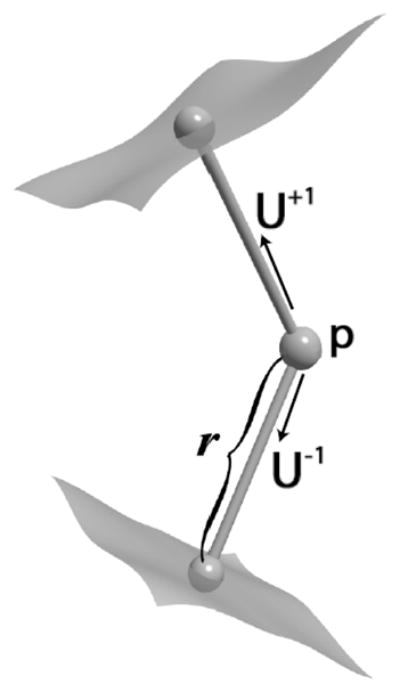
Medial atom: position (p), radius (r), two normals to boundary (U)

To obtain m-reps describing the subcortical structures in our study, we started with binary image segmentations from well-trained experts using semi-automated procedures.¹ We also needed an initial m-rep that would be deformed to fit the binary image. We constructed these initial medial models using the modeling scheme developed by Styner et al. [31] to determine the minimum sampling required for each model. Given a binary segmentation and initial model, the initial model is deformed through an optimization process such that the model best fits the image without becoming too irregular in its geometry [33]. This process is applied individually to each of the 10 anatomical objects using the Pablo tool [34], while the correspondence across samples is implicitly established by the deformation process on the template model. Fig. 2 shows the medial atoms for a set of objects (a) and the implied surfaces (b).

C. Alignment and Pose

In a multi-object setting, it must be decided how to remove unimportant shape variability through alignment. We call aligning the object set as a whole, where transformations are applied to all objects jointly, a global alignment. As seen in Fig. 3a and b, after this global alignment there are still local pose differences among the individual objects. In our case, we assumed these single object pose differences were important because they represent the inter-object changes within the multi-object set. Therefore, after the global alignment, we perform a second step referred to as the local alignment. In this step, we take the globally aligned object sets and align objects individually as would be done in a single object setting. It is these local pose changes that we include as part of the overall variability of the objects. The resulting m-reps after the local alignment are what we refer to as pure shape and can be seen in Fig. 3c. For the purposes of this paper, the global alignment included translation and rotation. This accounted for any pose differences between the original images. The local alignment included translation, rotation, and scale to remove all remaining pose. When we use the local pose changes as features for discriminant analysis, we have an 8-dimensional vector consisting of three elements for the translation, four for the orientation (stored as a quaternion), and one for the scale. After both global and local alignments have been finished, the final m-reps are in the mean pose position and are used as the pure shape features.

Fig. 3.

Multi-object alignment. a) Global translation and rotation. b) Global translation, rotation, and scale. c) Local translation, rotation, and scale after global translation and rotation.

To align m-reps, we use a slight variation of the standard Procrustes method [35]. In a normal Procrustes alignment on a set of boundary points, the sum-of-squared distances between corresponding points is minimized. The standard Euclidean distance serves as the metric. For our purposes, we instead minimize the geodesic distance between m-reps because they do not lie within a Euclidean space. The distance between two m-reps is then the sum of geodesic distances between their corresponding atoms. The geodesic distance d(m_a, m_b) between two medial atoms m_a and m_b equals

$$\left|\right|{\mathbf{p}}_b-{\mathbf{p}}_a,\frac{r_b}{r_a},\mathbf{R}({\mathbf{U}}_b^{+1})·{\mathbf{U}}_a^{+1},\mathbf{R}({\mathbf{U}}_b^{-1})·{\mathbf{U}}_a^{-1}\left|\right|$$ (1)

$$d(S_1,\dots ,S_N;M_1,\dots ,M_N)=\sum _{i=1}^N\sum _{j=1}^{i}d{(S_i·M_i,S_j·M_j)}^2$$ (2)

where R(x) is the rotation of x to (1,0,0), S_i, M_i are the i-th transformation and m-rep models. This results in the following steps:

1. Translations: First, the translational part of the alignment S_i is minimized (2) once and for all by centering each m-rep model. That is, each model is translated so that the average of its medial atoms positions is the origin.

2. Rotations and Scalings. The i-th m-rep model, M_i, is aligned to the mean of the remaining models, denoted μ_i. The alignment is accomplished by a gradient descent algorithm on SO(3) × R⁺ to minimize d(μ_i, S_i · M_i)². The gradient is approximated numerically by a central differences scheme. This is done for each of the models.

3. Iterate. Step 2 is repeated until the metric (2) cannot be further minimized. For more details, see [36].

D. Distance Weighted Discrimination

Discriminant analysis is concerned with finding the axis which best separates two populations. An optimization must be performed that somehow maximizes the distance between the discriminating axis and the data points while separating the two classes. It is formulated in a general way as follows (see Fig. 4): given points x_i, class indicators y_i ∈ {+1, −1}, and w the normal to the separating hyperplane, the distance or residual, r, from the points to the hyperplane is

Fig. 4.

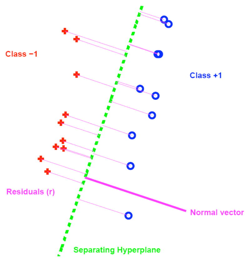
Illustration of two-class discrimination with separating hyperplane and residuals. The samples marked with boxes would act as the support vectors in SVM, whereas all samples are included in DWD.

$$r_i=y_i(x_i^{\prime }w+\beta )$$ (3)

where β determines the position of the hyperplane. One of the popular methods of discriminant analysis is Support Vector Machines (SVM). It attempts to maximize the minimum r_i. The main problem with this method is it tends to use only a small subset of the population, those near the opposite class, to completely define the discriminating axis. It is manifested in the problem of “data piling” (see Fig. 5) where most of the samples from the same population group, when projected onto the normal of the discriminating axis, end up very close to each other. This leads to poor generalization performance when tested on new samples that were not included in the calculation of the discriminating axis: it is too specific to the samples from which it was computed.

Fig. 5.

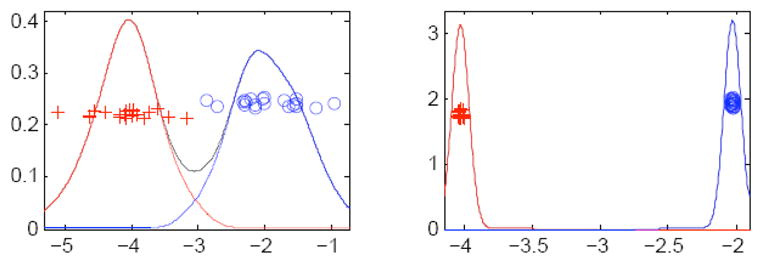
Left: Projection onto normal of optimal separating hyperplane. Right: Projection onto normal of separating hyperplane which exhibits data piling.

Distance weighted discrimination is a method similar to SVM, but uses all sample points in the calculation of the discriminating axis.² It attempts to minimize the sum of the reciprocals of r_i. Through this, each point’s contribution to the calculation is weighted proportionally to the distance from that point to the opposite population. In this way, the DWD achieves a higher robustness when presented with new, untrained samples. This advantage is heightened further in the context of high dimensional feature spaces with low sample sizes where it is best to use all information available from the low number of samples.

DWD was specifically developed for the high dimension low sample size setting (HDLSS). The shape analysis study presented in this paper is a good example of a HDLSS problem, as the dimensionality (1890 dimensional data, joint m-rep shape description of 10 subcortical structures) is much larger than the number of samples (70). Classical discrimination methodology based on Fisher Linear Discriminant is not appropriate in such as setting due to data overfitting and is usually outperformed by SVD or DWD.

E. Transformation of Raw Input Data

The m-rep shape description as well as the pose features contain rotational elements that are not part of a Euclidean space. This can lead to reduced performance of methods such as DWD that attempt to find a linear discriminant. Likewise, combining features with different units into one long feature vector can bias results towards features with larger variance. Finally, our data samples have unequal gender distributions within the two populations. We must first account for each of these issues before running DWD analysis.

While the application of DWD to nonlinear features may give a reasonable solution, we found through experimentation that the linearized form of the m-rep features gives a better discrimination result (see Fig. 6). To obtain a linear instance of our curvilinear m-rep and pose features, we project them into the tangent space at the geodesic mean point [36]. This involves taking the log map of each of the non-Euclidean features. For the pose rotation, the log map of a unit-length quaternion q = (w, v) is defined as

Fig. 6.

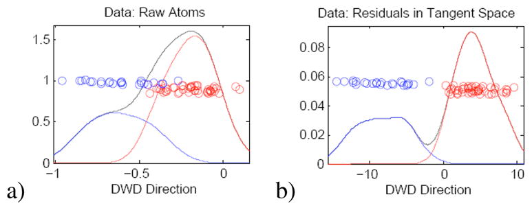
Separation of 70 multi-object m-reps into two populations given by DWD axis. a) Raw, nonlinear medial atom data. b) Atom data after projection into tangent space and subtraction of mean.

$$logq=\frac{\theta }{\mathit{sin}(\theta /2)}·\underset{\_}{\mathbf{v}},\theta =2\mathit{arccos}(w)$$ (4)

For the m-rep normal directions U = (x, y, z), the spherical log map is

$$log\mathbf{U}=\left(x·\frac{\theta }{\mathit{sin}(\theta )},y·\frac{\theta }{\mathit{sin}(\theta )}\right),\theta =\mathit{arccos}(z)$$ (5)

For the pose scale and m-rep radius factors it is just the logarithm function.

To concatenate features of differing units, we first must make them commensurate to avoid unwanted bias. For our purposes, we have chosen to normalize each feature by subtracting the mean and dividing by the standard deviation. This makes the weighting of points equal among separate features in the DWD calculation. So for each feature, the final input to the DWD routine is of the form

$$Y=\frac{X-\overline{X}}{\sigma }\forall X\in {\mathbb{R}}^k$$ (6)

$$Y=\frac{log(X-\overline{X})}{\sigma }\forall X\notin {\mathbb{R}}^k$$ (7)

The mean X̄, however, is computed for each gender. By subtracting a gender-specific mean, we eliminate any disproportion in the gender sampling within our two populations. To build a gender-specific mean, we start with the lowest level of subcategories within our data and compute the mean of the samples in each. We then compute the mean of the subcategory means which are of the same gender. This gives us a gender specific mean. Fig. 7 shows the process with subcategories according to the three criteria of gender, group, and time.

Fig. 7.

Illustration of gender-specific mean calculation given subcategories of gender, group, and time. The same process is applied to obtain a female mean.

F. Unbiased Classification using Leave-Many-Out Experiments

To test the performance of the DWD, we chose to implement a leave-many-out, cross-validation experiment. We first divided our data samples into a training set and a testing set. The discriminating axis was computed using the training set. Each sample from the test set was then projected onto the DWD axis with the resulting one-dimensional projected value serving as the classification score (hence known as the DWD score). The DWD method produces both a discriminating axis and a threshold β. The threshold value is the amount by which the training data, after projected onto the DWD, must be shifted such that zero becomes the best dividing point between populations. Therefore, given a DWD axis w and a test sample feature vector x, the DWD score becomes

$$s=x^{\prime }w+\beta$$ (8)

The discrete classification into one of the diagnosis groups is then simply the sign of the DWD score.

In order to make the training set unbiased, we used the following strategy for selecting training samples (see Algorithm 1). We would alternately choose a random autism or a random control sample. With this sample from one group, we chose the sample from the other group that was a best match according to age and gender to the subject from the first group. This gave us one sample from each group. Since our data is longitudinal, we always included each sample’s counterpart across time. From here, the process was repeated but starting with a random sample from the opposite group than in the previous iteration. After several iterations, we would have a training set with an equal number of samples from each group.

Algorithm 1.

Training Set T Selection

T = Ø, size = 0, i = 0 while size < n do  if i mod 2 = 0 then   s = random sample from autism group   t = closest matching sample to s from control group  else  s = random sample from control group  t = closest matching sample to s from autism group  end if  s′ = counterpart of s across time  t′ = counterpart of t across time  T = T ∪ {s, s′, t, t′}  size = size + 4  i = i + 1 end while

After several runs of this experiment, all of the data samples were included in the testing set of at least a few runs. From the results of these experiments, we could then build an unbiased estimate of each sample’s classification. For each sample, we computed it’s mean DWD score over those runs of the experiment for which it was in the test set. In this way, we calculate a classification for a sample only when the discriminating axis was computed without any knowledge of that sample. The box plots in the following sections are of these unbiased mean DWD scores.

As mentioned before, the study presented in this paper is based on a total of 70 samples with 46 autism and 24 control with information at age 2 and 4. There were four unpaired control samples, which were always left out of the training set. We chose the training set, in the manner described above, consisting of 32 out of the 70 available samples. It included 16 samples from the control group and 16 from the autism group. The remaining 38 samples served as the test set. The experiment was then run 100 times. The number of runs was chosen heuristically such that each of the 70 samples was included in the test set for at least a few runs; the minimum number of runs in the test set for any sample was 4. From these, we could calculate an unbiased mean DWD score.

As the two groups are not equally represented in the test set (30 autistic cases and 8 controls), we assess the discrimination accuracy of an individual test by averaging the discrimination accuracy of the two subgroups. Without averaging of the subgroups, a classifier that would always guess ’autism’ would result in a classification accuracy of 30/38 = 78.9%. Our average discrimination accuracy results for such a simple classifier in 50% classification accuracy.

III. Results

In this section, we describe the results of our discrimination based shape analysis experiments. We have divided the results into five sections corresponding to the features used in the discriminant analysis: volume, pose, shape, shape and pose combined, and m-rep radii. We then finish with some visualizations of the discriminating differences between the populations. The subdivision of the results was performed in order to study

A. Volume

Because of its prevalence in neuroimaging studies, we first assessed the ability of object volumes to discriminate between the autism and control groups. The volumes were computed from the implied surface boundary of the m-reps. The 10 subcortical structures gave us a 10-dimensional feature space to serve as the basis for the discriminating axis. We computed the mean DWD score for each sample over the runs in which that sample was in the test set. This gives us an unbiased average classification score for each sample. Fig. 8 shows that there is a clear difference between the median score of the autism group and control group. This difference is statistically significant with p<0.001. As another measure of the discrimination performance of the volume, Table I shows the average percentage (74%) of the 38 test samples that were correctly classified over the 100 runs of the leave-many-out experiment.

Fig. 8.

Volume features: Box plot (median, 25 and 75 percentiles, min/max) of mean DWD scores of each group over those runs in which the samples were in the test set. Greater than zero classified as autism, less than zero classified as control. p<0.001.

TABLE I.

Classification Accuracies for Test Samples over 100 Runs of Leave-Many-Out Experiment

Feature	Mean	Std. Dev.
Volume	74 %	± 8 %
Pose	57 %	± 9 %
Pose (Scale Only)	64 %	± 7 %
Shape	56 %	± 8 %
Shape and Pose	55 %	± 8 %
Shape and Scale (Radii Only)	76 %	± 7 %

B. Pose

The next step was to explore the significance of local pose changes. For each sample, these features totaled 70: three for translation, three for rotation, and one for uniform scale across 10 objects. The raw features were transformed as described above, thus reducing the quaternion representing the rotation to a three-dimensional vector. The significance in the volume discrimination led us to believe that the pose, which includes uniform object scale factors, would also show significance. This was the case for the mean DWD scores with p=0.03 (Fig. 9). However, the test sample classification accuracy was considerably lower than volume as Table I illustrates.

Fig. 9.

Pose features: Box plot (median, 25 and 75 percentiles, min/max) of mean DWD scores of each group over those runs in which the samples were in the test set. Greater than zero classified as autism, less than zero classified as control. p=0.03.

There also were 20 individual runs in which the classification accuracy was at or below 50%, a result that would be outperformed by a random coin flip. The translation and rotation components of the pose seemed to be adding mostly noise and instability to the DWD calculation because the same experiment run with only the scale factors gave an average classification rate of 64% and p=0.002 as opposed to 54% and p=0.1 using the translations and rotations. From these results, we conclude that the pose does include some relevant information for discrimination but it is likely in the uniform scale factors. The classification rate of volume (74%) compared with the scale factors (64%) is illustrative of shape based uniform scaling factors not capturing full information of volumetric measurements.

C. Shape

Fig. 10 shows the results of using only the m-rep shape features for the DWD calculations. As with volume and pose, the mean DWD scores for the test samples were significantly different (p=0.01, Fig. 10). The classification accuracy of shape was equal to pose with an average correctness rate of 56%. The DWD methodology proved its usefulness and stability in high dimensional low sample size settings here because the m-rep shape features for the 10 subcortical structures number about 2000 in total, whereas the volume and pose were 10 and 70 respectively. Even in this high dimensional space, the DWD still generalized well enough to equal the performance of the pose features.

Fig. 10.

Shape features: Box plot (median, 25 and 75 percentiles, min/max) of mean DWD scores of each group over those runs in which the samples were in the test set. Greater than zero classified as autism, less than zero classified as control. p=0.01.

D. Shape and Pose

Finally, the high classification accuracy of the volumes compared with both the shape and pose features led us to combine the latter two. This gave us the most complete description of the variability of the multi-object complex. The differences between the mean DWD scores were not significant (p=0.38). Once again, the pose features seem to be mostly noise since combining them with shape produced a nonsignificant result while shape alone was significant. The classification accuracy (55%) was similar to the shape and pose features individually as seen in Table I.

E. Shape and Scale: M-rep Radii

One of the ongoing questions with a discretely sampled m-rep shape description is the issue of correspondence. Currently, the correspondence is implicitly defined in the process of fitting a template model to each binary image. However, it is not clear that features such as the spokes and atom positions are sufficiently stable to give a meaningful correspondence across samples. Out of this arises the question of whether statistics on these features, which we used as part of our shape analysis above, could be tighter with a better correspondence.

To explore this question, we chose to run our same analysis on only the radius feature of each medial atom without any alignment. This is because the radius is less sensitive to a noisy correspondence than some of the other medial atom features; a small change in the atom position or spoke directions will generally not cause a large change in the radius. It is also invariant to any object-level translation and rotation, while including both shape and scale information in the form of local width. This makes it a more intrinsic measure than the other medial atom features. Compared to the other features in Table I, the mean classification accuracy over 100 runs of the leave-many-out experiment is best when using only the atom radii at 76%. Fig. 12 shows the mean DWD scores using only the radii. While the radii give the best classification rate of any feature we studied, it is difficult to say outright that they are the best features to use. First, it may be our specific application that lends itself to a local measure that is related to volume like the radii. It is known, and evidenced above, that there are volume differences between autistic and typically developing brains. Also, Fig. 12 shows that the overlap between the populations is not drastically better than with volume. However, the jump in classification accuracy from using all the medial atom features to only the radii suggests that there is a certain amount of noise in the other features which ends up being correlated to the detriment of the DWD calculation. At the same time, witnessing the radii outperform volume as a discriminating feature adds validation to our general choice of the medial shape representation.

Fig. 12.

M-rep radii features: Box plot (median, 25 and 75 percentiles, min/max) of mean DWD scores of each group over those runs in which the samples were in the test set. Greater than zero classified as autism, less than zero classified as control. p<0.001.

F. Evaluation of Bias

To verify that the mean classification scores were unbiased, we ran our same experiments using random, normally distributed input data. We used the same random number seeding and the exact same training and testing sets. The random data was generated with the same mean, variance, and dimension as our actual shape data. The p-value of the mean DWD scores for this case was 0.22 and the average classification accuracy was 49%.

G. Discrimination by Age

To complete our analysis, we ran the same experiments as above, with precisely the same gender-corrected data, but discriminating according to age instead of diagnosis. Through this we wanted to explore the performance of the discrimination in the context of presumably more separate groups. And indeed, as seen in Table II, most of the different features have an easier time discriminating by age than by diagnosis. Especially noteworthy is the pose, which does marginally better than the volume, m-rep radii, and scale factors (see Figs. 13 and 14). It is important to remember that the latter two are not a total brain volume or scale, which should be easily separated after correcting for gender, but for the individual structures. Our previous work [37] had shown that the first principal mode of our pooled data (both time points) aligned very closely with time. The deformation along this mode showed a large global scaling effect, with the subcortical structures moving radially outward. Here, this change across time is represented in the local translation alignment parameters, which helps to explain why the entire local pose (translation, rotation, and scale) performs slightly better than scale or volume alone. Our conclusion is that since pose does well at discriminating by age, removing it for the analysis of diagnosis groups (and witnessing it not aid in the discrimination when included) leaves us with discriminating differences that are not heavily influenced by having pooled data across time. However, a direct method of correcting for age, such as that done for gender, would be preferable and will be explored in the future.

TABLE II.

Classification Accuracies for Discrimination by Age

Feature	Mean	Std. Dev.
Volume	72 %	± 5 %
Pose	74 %	± 6 %
Pose (Scale Only)	72 %	± 6 %
Shape	64 %	± 6 %
Shape and Pose	72 %	± 6 %
Shape and Scale (Radii Only)	70 %	± 6 %

Fig. 13.

Pose features (by age): Box plot (median, 25 and 75 percentiles, min/max) of mean DWD scores of each group over those runs in which the samples were in the test set. Greater than zero classified as autism, less than zero classified as control.

Fig. 14.

M-rep radii features (by age): Box plot (median, 25 and 75 percentiles, min/max) of mean DWD scores of each group over those runs in which the samples were in the test set. Greater than zero classified as autism, less than zero classified as control.

H. Visualization

To visualize the changes in shape along the DWD direction, we start with the mean m-rep of the autism group. Then, we deform the autism mean m-rep along the unit-length DWD which points toward the control group. The distance along the DWD direction by which the autism mean is deformed is defined as the distance between the mean of each group’s projections onto the DWD line. The final m-rep which has been deformed this full distance is then used to represent the control group.

For robustness, we chose to use the mean DWD direction over all the runs instead of using a single run from the leave-many-out experiment. We also used all 70 samples to compute the distance between the projected group means, which gives us the distance to deform along the DWD direction, and all 46 autism samples for the autism mean m-rep. Fig. 15a shows colormaps of surface distances between the two multi-object sets representing each of the two diagnosis groups using shape only. The measurement is the distance when starting from the autism group and deforming towards the control group. Red, green, and blue coloring denote inward, zero, and outward deformations respectively. In this image, we see that the amygdala and hippocampus undergo strong shape changes between the groups relative to the other three structures. There is a distinct inward deformation of the hippocampus tail (seen in far right of Fig. 15a) as well as an outward change in the midsection. A large portion of each amygdala also presents a difference in shape.

Fig. 15.

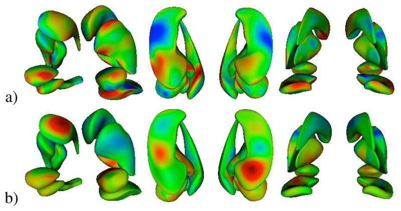
Colormap of surface distances from autism mean m-rep to deformed m-rep along DWD direction using a) shape only, b) m-rep radii only. Red, green, and blue are inward distance, zero distance, and outward distance respectively.

Given that the m-rep radii performed best as a discriminating feature, we also wanted to visualize these differences. We used the same procedure as above to obtain a representative set of radii for each diagnosis group. Fig. 15b shows the surface distance between m-reps of each group with only the radii modified. The strongest individual radii changes appear to be in the hippocampus and the caudate. To assess the overall radii differences between groups, we calculated Δr = log (r_c/r_a) for each corresponding atom with r_c the radius of the control group and r_a the radius of the autism group. Fig. 16 shows spheres plotted at the mean atom positions between the two groups with size proportional to Δr. The color denotes the sign of Δr, with red being a decrease in radius from autism to control and blue an increase. We see a clear decrease in local widths when deforming from autism to control at almost all positions across the three structures. Both the hippocampus and caudate show decreases in the posterior head with slight increases in the body section. These overall radii decreases are supported by Table III which lists the percent change from autism to control of the mean volumes of each structure at ages 2 and 4. All structures show a larger volume in the autism group.

Fig. 16.

Visualization of radii change from autism to control in a) right amygdala, b) right hippocampus, c) right caudate. Size of ball at an atom position is proportional in size to the log of the control’s radius minus the log of the autism’s radius. Red is an increase in radius from autism to control and blue is a decrease.

TABLE III.

Volume Percent Change from Autism to Control

Object	%Δ2	%Δ4
Left Amygdala	−19.85	−15.41
Right Amygdala	−21.05	−18.19
Left Caudate	−14.38	−3.84
Right Caudate	−13.96	−5.49
Left Hippocampus	−10.92	−7.98
Right Hippocampus	−10.29	−6.69
Left Globus Pallidus	−10.19	−16.17
Right Globus Pallidus	−2.57	−8.27
Left Putamen	−6.43	−3.66
Right Putamen	−4.54	−2.24

$\%{\mathrm{\Delta }}_A=\frac{{\overline{\mathit{Vol}}}_{\mathit{cont}}-{\overline{\mathit{Vol}}}_{\mathit{aut}}}{{\overline{\mathit{Vol}}}_{\mathit{cont}}}\times 100$, at age A

IV. Discussion and Conclusion

This research demonstrates work in progress towards shape analysis and group discrimination of multi-object complexes. Traditionally, shape analysis is mostly concerned with representation and statistical analysis of single objects, mostly following a well developed mathematical framework that proposes linear alignment and subsequent statistical analysis of corresponding features.

In a multi-object setting, the alignment step has to be reconsidered as a critical choice. Linear alignment of a population of sets of objects will remove global translation, rotation and scale, but will not account for relative object pose variability. A joint analysis of only globally aligned sets of shapes will therefore include these residual pose differences into the statistical shape model. Here, we discuss and explore the various options for global and local alignment of sets of shapes. We propose an initial global alignment with rotation and translation to map each dataset into a common coordinate frame. This step is followed by a local alignment of each object individually, but the alignment parameters translation, rotation and scale are kept as pose parameter vectors. Shape analysis of the joint set of objects will therefore use pure shape features not affected by any residual pose differences. Features are mapped into Riemannian symmetric space, the appropriate choice for medial atom features that include rotational frames and positive reals, and are ready for statistical analysis. The same technique can be applied to the vectors of the joint pose parameters of the multi-object complexes. It is then straightforward to chose pose, shape, or pose and shape as features for group discrimination. Alternatively to the stepwise feature selection procedure presented in this manuscript, one could also use an automatic feature selection approach. The focus here though is on understanding the interaction of pose and shape features in the multi-object settings, as compared to generating the best pose and shape feature set.

Our results show that in this specific application, pose features do not give statistically significant discrimination. Shape features also did not show significance, except when isolating a particular feature of the m-rep shape description, namely the radius measure of local width. This feature combines the locality of a shape description with the scale information known to be discriminating in our particular application, which results in better generalized discrimination performance.

Although sampled medial representations use a lower number of features than densely sampled surfaces, we still face the HDLSS problem (high dimensionality low sample size). This problem is even more pronounced with the analysis of object sets, resulting in a feature space dimensionality which is magnitudes larger than the number of samples. In typical applications similar to the one described here, two populations of 25 samples are each represented by approximately 2000 features to provide a sufficiently detailed representation for 10 3-D objects. For classification, we applied the distance-weighted discrimination (DWD) method, which is a variant of support vector machine discrimination but is designed to be robust for HDLSS data analysis problems. Classifiers other than DWD but suited in the HDLSS setting could be chosen as well, and we make no claim that the best classification method was chosen here. Nevertheless, in our shape analysis studies DWD has shown to outperform classic SVM with respect to stability and classification rate. Unbiased statistical analysis by repeated leave-many-out experiments finally results in classification rates and significance values (p-values).

The driving application is a pediatric autism study with autistic and typically developing children imaged at 2 and 4 years of age. We focus on a joint analysis of five left and right subcortical structures represented as sampled medial representations after model fitting. Please note the discrepancy of relatively low classification rates in the presences of highly significant population differences. This might possibly be explained by the nature of the underlying clinical problem. Morphologic phenotypes in neurodevelopmental disorders are often reflected by only subtle differences and increased heterogeneity. Discrimination rates in psychiatric pathology such as autism or schizophrenia are commonly low, as the overlap between normal anatomy and changes due to pathology is considerable. Near perfect discrimination rates would be very suspicious of overfitting.

The results fit well with the current literature on autism [32]. Shape analysis differences previously found on the hippocampus [38] correlate well with our findings shown in Figure 16 (enlargement in head and tail sections and reduction in the body section). Overall volumetric differences in caudate and amygdala have been reported [39][40], but no shape analysis studies have yet been performed on these structures.

In the future, we will explore multi-variate classification by selection of a best-separating subspace rather than a single axis. Further, we will have to develop a technique to explore the covariance structure of sets of shapes in order to explain their interrelationship. This will help clinicians to explore links between morphological changes and underlying biological processes.

Fig. 11.

Shape and pose features combined: Box plot (median, 25 and 75 percentiles, min/max) of mean DWD scores of each group over those runs in which the samples were in the test set. Greater than zero classified as autism, less than zero classified as control. p=0.38.

References

- 1.Thomson D. On Growth and Form. 2. Cambridge University Press; 1942. [Google Scholar]
- 2.Dryden I, Mardia K. Multivariate shape analysis. Sankhya. 1993;55:460–480. [Google Scholar]
- 3.Small CG. The statistical theory of shape. Springer; 1996. [Google Scholar]
- 4.Litvin A, Karl WC. Coupled shape distribution-based segmentation of multiple objects. Information Processing in Medical Imaging. 2005:345–356. doi: 10.1007/11505730_29. [DOI] [PubMed] [Google Scholar]
- 5.Dryden I, Mardia K. Statistical Shape Analysis. Wiley; 1998. [Google Scholar]
- 6.Marron J, Todd M. “Distance weighted discrimination,” Operations Research and Industrial Engineering, Cornell University. Technical Report. 2002;1339 available at http://www.stat.unc.edu/postscript/papers/marron/HDD/DWD/DWD2.pdf.
- 7.Golland P, Grimson WEL, Shenton ME, Kikinis R. Detection and analysis of statistical differences in anatomical shape. Medical Image Analysis. 2005;9:69–86. doi: 10.1016/j.media.2004.07.003. [DOI] [PMC free article] [PubMed] [Google Scholar]
- 8.Yushkevich P, Pizer SM, Joshi S, Marron J. Intuitive, localized analysis of shape variability. Information Processing in Medical Imaging. 2001:402–408. [Google Scholar]
- 9.McCarley R, Wible C, Frumin M, Hirayasu Y, Levitt J, Fischer I, Shenton M. Mri anatomy of schizophrenia. Biological psychiatry. 1999 doi: 10.1016/s0006-3223(99)00018-9. [DOI] [PMC free article] [PubMed] [Google Scholar]
- 10.Levitt J, McCarley R, Dickey C, Voglmaier M, Niznikiewicz M, Seidman L, Hirayasu Y, Ciszewski A, Kikinis R, Jolesz F, Shenton M. Mri study of caudate nucleus volume and its cognitive correlates in neuroleptic-naive patients with schizotypal personality disorder. Am J Psychiatry. 2002;159(7):1190–1197. doi: 10.1176/appi.ajp.159.7.1190. [DOI] [PMC free article] [PubMed] [Google Scholar]
- 11.Keefe RSE, Seidman LJ, Christensen BK, Hamer RM, Sharma T, Sitskoorn MM, Rock SL, Woolson S, Tohen M, Tollefson GD, Sanger TM, Lieberman JA. Long-term neurocognitive effects of olanzapine or low-dose haloperidol in first-episode psychosis. Biological psychiatry. 2006;59(2):97–105. doi: 10.1016/j.biopsych.2005.06.022. [DOI] [PubMed] [Google Scholar]
- 12.Juranek J, Filipek PA, Berenji GR, Modahl C, Osann K, Spence MA. Association between amygdala volume and anxiety level: magnetic resonance imaging (mri) study in autistic children. Journal of child neurology. 2006 Dec;21(12):1051–8. doi: 10.1177/7010.2006.00237. [DOI] [PubMed] [Google Scholar]
- 13.Langen M, Durston S, Staal WG, Palmen SJMC, van Engeland H. Caudate nucleus is enlarged in high-functioning medication-naive subjects with autism. Biol Psychiatry. 2007 doi: 10.1016/j.biopsych.2006.09.040. [DOI] [PubMed] [Google Scholar]
- 14.Munson J, Dawson G, Abbott R, Faja S, Webb SJ, Friedman SD, Shaw D, Artru A, Dager SR. Amygdalar volume and behavioral development in autism. Archives of general psychiatry. 2006 June;63(6):686–93. doi: 10.1001/archpsyc.63.6.686. [DOI] [PubMed] [Google Scholar]
- 15.Styner M, Lieberman A, McClure RK, Weinberger DR, Jones DW, Gerig G. Morphometric analysis of lateral ventricles in schizophrenia and health controls regarding genetic and disease-specific factors. Proc of the National Academy of Sciences. 2005 March;102(13):4872–4877. doi: 10.1073/pnas.0501117102. [DOI] [PMC free article] [PubMed] [Google Scholar]
- 16.Gerig G, Styner M, Shenton M, Lieberman J. Shape versus size: Improved understanding of the morphology of brain structures. MICCAI. 2001:24–32. [Google Scholar]
- 17.Bossa MN, Olmos S. Statistical model of similarity transformations: Building a multi-object pose. 2006 Conference on Computer Vision and Pattern Recognition Workshop (CVPRW’06); 2006. p. 59. [Google Scholar]
- 18.Bookstein F. Shape and the information in medical images: A decade of the morphometric synthesis. MMBIA. 1996 [Google Scholar]
- 19.Cootes T, Taylor C, Cooper D, Graham J. Active shape models -their training and application. Comp Vis Image Under. 1995;61:38–59. [Google Scholar]
- 20.Kelemen A, Székely G, Gerig G. Elastic model-based segmentation of 3d neuroradiological data sets. IEEE Trans Med Imaging. 1999;18:828–839. doi: 10.1109/42.811260. [DOI] [PubMed] [Google Scholar]
- 21.Staib L, Duncan J. Model-based Deformable Surface Finding for Medical Images. IEEE Trans Med Imaging. 1996;15(5):1–12. doi: 10.1109/42.538949. [DOI] [PubMed] [Google Scholar]
- 22.Tsai A, Yezzi A, Wells W, Tempany C, Tucker D, Fan A, Grimson E, Willsky A. Shape-based approach to curve evolution for segmentation of medical imagery. IEEE Transactions on Medical Imaging. 2003 Feb;22(2):137–154. doi: 10.1109/TMI.2002.808355. [DOI] [PubMed] [Google Scholar]
- 23.Yang J, Staib LH, Duncan JS. Neighbor-constrained segmentation with level set based 3d deformable models. IEEE Transactions on Medical Imaging. 2004 Aug;23(8):940–948. doi: 10.1109/TMI.2004.830802. [DOI] [PMC free article] [PubMed] [Google Scholar]
- 24.Davatzikos C, Vaillant M, Resnick S, Prince J, Letovsky S, Bryan R. A computerized method for morphological analysis of the corpus callosum. J of Comp Assisted Tomography. 1996 Jan./Feb;20:88–97. doi: 10.1097/00004728-199601000-00017. [DOI] [PubMed] [Google Scholar]
- 25.Csernansky J, Joshi S, Wang L, Haller J, Gado M, Miller J, Grenander U, Miller M. Hippocampal morphometry in schizophrenia via high dimensional brain mapping. Proc Natl Acad Sci USA. 1998 September;95:11 406–11 411. doi: 10.1073/pnas.95.19.11406. [DOI] [PMC free article] [PubMed] [Google Scholar]
- 26.Thompson P, Mega M, Toga A. ch Disease-Specific Brain Atlases. Academic Press; 2000. Brain Mapping: The Disorders. [Google Scholar]
- 27.Thompson P, Giedd J, Woods R, MacDonald D, Evans A, Toga A. Growth patterns in the developing brain detected by using continuum mechanical tensor maps. Nature. 2000;404:190–193. doi: 10.1038/35004593. [DOI] [PubMed] [Google Scholar]
- 28.Pizer S, Fritsch D, Yushkevich P, Johnson V, Chaney E. Segmentation, registration, and measurement of shape variation via image object shape. IEEE Trans Med Imaging. 1999;18:851–865. doi: 10.1109/42.811263. [DOI] [PubMed] [Google Scholar]
- 29.Styner M, Lieberman JA, Pantazis D, Gerig G. Boundary and medial shape analysis of the hippocampus in schizophrenia. MedIA. 2004:197–203. doi: 10.1016/j.media.2004.06.004. [DOI] [PubMed] [Google Scholar]
- 30.Bouix S, Pruessner JC, Collins DL, Siddiqi K. Hippocampal shape analysis using medial surfaces. NeuroImage. 2005;25:1077–1089. doi: 10.1016/j.neuroimage.2004.12.051. [DOI] [PubMed] [Google Scholar]
- 31.Styner M, Gerig G, Lieberman J, Jones D, Weinberger D. Statistical shape analysis of neuroanatomical structures based on medial models. Medical Image Analysis (MEDIA) 2003 Sept;7(3):207–220. doi: 10.1016/s1361-8415(02)00110-x. [DOI] [PubMed] [Google Scholar]
- 32.Hazlett HC, Poe MD, Gerig G, Smith RG, Piven J. Cortical gray and white brain tissue volume in adolescents and adults with autism. Biol Psychiatry. 2006 Jan;59(1):1–6. doi: 10.1016/j.biopsych.2005.06.015. [DOI] [PubMed] [Google Scholar]
- 33.Pizer S, Fletcher T, Fridman Y, Fritsch D, Gash A, Glotzer J, Joshi S, Thall A, Tracton G, Yushkevich P, Chaney E. Deformable m-reps for 3d medical image segmentation. International Journal of Computer Vision IJCV. 2003;55(2):85–106. doi: 10.1023/a:1026313132218. [DOI] [PMC free article] [PubMed] [Google Scholar]
- 34.Pizer SM, Fletcher PT, Joshi S, Gash AG, Stough J, Thall A, Tracton G, Chaney EL. A method and software for segmentation of anatomic object ensembles by deformable m-reps. Medical Physiscs Journal. 2005 May;32(5):1335–1345. doi: 10.1118/1.1869872. [DOI] [PubMed] [Google Scholar]
- 35.Goodall C. Procrustes methods in the staistical analysis of shape. Journal of the Royal Statistical Society. 1991;53(2):285–339. [Google Scholar]
- 36.Fletcher P, Lu C, Pizer S, Joshi S. Principal geodesic analysis for the study of nonlinear statistics of shape. IEEE Transactions on Medical Imaging. 2004;23:995–1005. doi: 10.1109/TMI.2004.831793. [DOI] [PubMed] [Google Scholar]
- 37.Styner M, Gorczowski K, Fletcher T, Jeong J, Pizer SM, Gerig G. Multi-object statistics using principal geodesic analysis in a longitudinal pediatric study. In: Yang G-Z, Jiang T, Shen D, Gu L, Yang J, editors. Lecture Notes in Computer Science; MIAR Conference; Aug, 2006. pp. 1–8. [Google Scholar]
- 38.Dager SR, Wang L, Friedman SD, Shaw DW, Constantino JN, Artru AA, Dawson G, Csernansky JG. Shape mapping of the hippocampus in young children with autism spectrum disorder. AJNR American journal of neuroradiology. 2007;28:672–7. [PMC free article] [PubMed] [Google Scholar]
- 39.Amaral DG, Schumann CM, Nordahl CW. Neuroanatomy of autism. Trends Neurosci. 2008 Mar;31(3):137–45. doi: 10.1016/j.tins.2007.12.005. [DOI] [PubMed] [Google Scholar]
- 40.Stanfield AC, McIntosh AM, Spencer MD, Philip R, Gaur S, Lawrie SM. Towards a neuroanatomy of autism: a systematic review and meta-analysis of structural magnetic resonance imaging studies. Eur Psychiatry. 2008 Jun;23(4):289–99. doi: 10.1016/j.eurpsy.2007.05.006. [DOI] [PubMed] [Google Scholar]