ACOUSTIC RADIATION FORCE-DRIVEN ASSESSMENT OF MYOCARDIAL ELASTICITY USING THE DISPLACEMENT RATIO RATE (DRR) METHOD

Abstract

A noninvasive method of characterizing myocardial stiffness could have significant implications in diagnosing cardiac disease. Acoustic radiation force (ARF)–driven techniques have demonstrated their ability to discern elastic properties of soft tissue. For the purpose of myocardial elasticity imaging, a novel ARF-based imaging technique, the displacement ratio rate (DRR) method, was developed to rank the relative stiffnesses of dynamically varying tissue. The basis and performance of this technique was demonstrated through numerical and phantom imaging results. This new method requires a relatively small temporal (<1 ms) and spatial (tenths of mm²) sampling window and appears to be independent of applied ARF magnitude. The DRR method was implemented in two in vivo canine studies, during which data were acquired through the full cardiac cycle by imaging directly on the exposed epicardium. These data were then compared with results obtained by acoustic radiation force impulse (ARFI) imaging and shear wave velocimetry, with the latter being used as the gold standard. Through the cardiac cycle, velocimetry results portray a range of shear wave velocities from 0.76–1.97 m/s, with the highest velocities observed during systole and the lowest observed during diastole. If a basic shear wave elasticity model is assumed, such a velocity result would suggest a period of increased stiffness during systole (when compared with diastole). Despite drawbacks of the DRR method (i.e., sensitivity to noise and limited stiffness range), its results predicted a similar cyclic stiffness variation to that offered by velocimetry while being insensitive to variations in applied radiation force.

INTRODUCTION

Cardiac stiffness

In 2006, 34% of all deaths in the United States were caused by cardiovascular disease (Lloyd-Jones et al. 2010). In that same year, 8.5 million Americans had a myocardial infarction and 5.8 million had heart failure. These forms of cardiac disease, as well as others, often manifest themselves as changes in myocardial stiffness. Freshly infarcted myocardium, in addition to losing its contractility, becomes significantly stiffer and remains stiff during later phases of healing (Holmes et al. 2005). Diastolic heart failure is associated with the inability of the ventricles to sufficiently relax (i.e., decrease in stiffness) during diastole, whereas systolic heart failure represents a failure of the heart to sufficiently contract (and thus stiffen) during systole (Zile et al. 2004; Vasan and Levy 2000). Consequently, a noninvasive, inexpensive and effective means of assessing myocardial stiffness through the cardiac cycle could be of diagnostic value.

Because stiffness captures the relationship between stress and strain within a medium, many groups have focused on quantifying strain—which in the heart tends to be easier to estimate than its stress counterpart—to indirectly assess cardiac function. To this end, researchers have focused on naturally occurring or externally generated dynamics, whereas motion tracking methods to assess strain have used both ultrasound-based and magnetic resonance imaging (MRI)–based techniques (Fatemi and Greenleaf 2002). The cyclic contraction of the heart’s chambers results in cyclic variations in chamber volume, pressure and wall strain. An assessment of chamber stiffness can be achieved through a chamber’s P-V loop, which typically involves estimating its pressure-volume relationship over multiple heartbeats during an increase in blood pressure (Mirsky et al. 1987). This method generally requires invasive, catheter-based techniques for pressure and volume (i.e., conductance catheter) estimates. An ultrasound-based approach, strain or strain-rate imaging permits one to track regional deformations in the heart with conventional ultrasonic methods (Amundsen et al. 2006; D’hooge et al. 2002); this analysis can then be used to assess wall elasticity changes associated with ischemic/reperfused myocardium (Pislaru et al. 2004). The underlying simplifications and assumptions, however, in tissue geometry and distribution of loads can make estimation of cardiac function based on strain and strain-rate imaging susceptible to artifacts (Burkhoff et al. 2005).

In addition to tracking gross wall motion, it is also possible to track naturally occurring, low-frequency waves traversing the myocardium. Kanai (2005) first investigated mechanical waves generated by the transient dynamics of aortic valve closure. He measured wave speeds in the intraventricular septum (IVS) of 2.0–4.5 m/s during early diastole. Citing a wavelength that was larger than the IVS wall thickness, Kanai used a mechanical model based on Lamb wave propagation to derive specific elasticity metrics (i.e., stiffness and viscosity). This technique, however, requires valve closure and thus cannot be applied throughout the cardiac cycle. In addition to naturally occurring phenomena, one can also create a wave through external means. If a low-frequency, external, harmonic excitation is coupled into the heart, an MRI-based elasticity imaging technique, known as magnetic resonance elastography (MRE), can be implemented (Muthupillai et al. 1995). Rump et al. (2007) generated 50-Hz mechanical waves in the IVS of a human heart with an external rod. The speed of these waves was measured with MRE to be 2.5 ± 0.4 m/s; no significant changes in velocity through the cardiac cycle were found. Using a plate model, they predicted elasticities of 27–5 kPa from late diastole to systole, respectively. Sack et al. (2009) used a similar protocol, but with a 25-Hz excitation, to measure a shear modulus ratio (diastole:systole) of 37.7 ± 10.6 throughout the cardiac cycle. Given the current cost of MRI-based scanning, however, it is unlikely such a technique will experience widespread clinical implementation.

ARFI-based imaging

ARF is generated whenever an acoustic wave interacts with absorbing or reflecting elements in its propagation path (Torr 1984). This force results from a transfer of momentum and is in the direction of wave propagation for the case of pure absorption, a condition often approximated for soft tissue (Westervelt 1951; Lyons and Parker 1988). If a plane wave assumption is made (in addition to the pure absorption assumption), the force application at a specific point is proportional to the absorption coefficient and time-average intensity at that point (Nyborg 1965). If an ARF application is of short duration (e.g., <1 ms), it is often referred to as an ARF impulse (ARFI). When an ARFI is generated in soft tissue, micron-order displacement away from the transducer results after force application in the region of ultrasonic beam propagation. Slightly later in time (i.e., typically in ms), displacement is generated at laterally offset locations because of the production of shear waves, which travel in the direction transverse to longitudinal wave propagation (Sarvazyan et al. 1998). In a linear, isotropic, elastic medium, the speed of these shear waves can be expressed as (Lai et al. 1993):

$$c_t=\sqrt{\frac{\mu }{\rho }}=\sqrt{\frac{E}{2(1+v)\rho }},$$ (1)

where μ is the shear modulus, E is the Young’s modulus, v is the Poisson’s ratio and ρ is the density of the tissue. This relationship demonstrates that shear wave velocity is proportional to a tissue’s stiffness. A typical range for shear wave velocities in soft tissue is 1–5 m/s (Bishop et al. 1998).

Using the ARFI-induced dynamics that occur on-axis (within the ARF beam profile) and off-axis (outside the beam profile and caused by shear wave propagation), it is possible to incorporate ARFI pulses (i.e., with pulse lengths typically 50 to 100 μs) into ultrasound sequences for the purpose of elasticity imaging. The peak displacement achieved on-axis and resulting from an ARFI pulse is inversely related to tissue stiffness (Palmeri et al. 2005). Multiple research groups have used an on-axis approach, commonly referred to as ARFI imaging, for the purpose of characterizing viscoelastic elements of breast, liver and vascular disease (Nightingale et al. 2001; Melodelima et al. 2006; Behler et al. 2009; Palmeri et al. 2008). Off-axis dynamics can be investigated for similar purposes. Such an imaging approach, commonly referred to as shear wave elasticity imaging (SWEI), relies on the relationship presented in eqn (1) and enables quantification of a tissue’s stiffness modulus if an elasticity model is assumed (Bercoff et al. 2004; Sarvazyan et al. 1998; Nightingale et al. 2003). In this paper, because of the complex material and structural properties of the heart, rather than making simplifying assumptions, we report only shear wave speeds, which will be referred to as “shear wave velocimetry” or simply “velocimetry.”

Using ARFI imaging, Hsu et al. (2007) observed evidence of in vivo cyclic stiffness variation of the left ventricular free wall (LVFW) by imaging directly on the epicardium. By quantifying the displacement 0.7 ms after initiation of the ARFI excitation, they measured an average ratio between maximum diastolic to minimum systolic displacement of 5.3:1. They reasoned that the increased (ARFI-induced) displacement occurring during diastole suggested a period of greater compliance when compared with periods of lesser displacement during systole. This cyclic variation in induced displacement, however, could be affected by variations in absorption and/or scattering (both of which result in commensurate variations in ARF) throughout the cardiac cycle. Madaras et al. (1983) measured a difference of 3.5 dB in integrated myocardial backscatter through the cardiac cycle of a canine heart. Although a precise measurement has yet to be achieved, the myocardial absorption coefficient could likewise vary throughout the cycle. Changes in scattering or absorption throughout the cardiac cycle would result in variation in ARFI-induced displacement that would not necessarily be stiffness dependent. Using a similar experimental setup to that used by Hsu et al. (2007) but relying on velocimetry, Bouchard et al (2009b) generated mechanical waves in the LVFW of an in vivo canine heart during diastole and measured wave speeds that ranged from 0.82–2.65 m/s. Successfully implementing such an approach in a clinical setting, however, would be challenging. If velocimetry is to be achieved in the heart, the method’s increased sampling times (milliseconds to tens of milliseconds) could prove to be too long for certain points of the cardiac cycle, during which uniaxial tissue velocities in excess of 25 mm/s during both systole and diastole are observed (Gorcsan et al. 1996). In addition, lateral motion could jeopardize the assumed spatial continuity of the method’s relatively large data kernels (3.2 mm² in this study).

In this study, a new on-axis approach, the displacement ratio rate (DRR) method, is presented and validated through simulation and phantom studies. Similar ARFI imaging and velocimetry techniques as those implemented by Hsu et al. (2007) and Bouchard et al. (2009b) are then used in an in vivo canine heart study for comparison. As the results will demonstrate, the DRR method provides a relative indication of myocardial stiffness changes throughout the cardiac cycle but requires, when compared with velocimetry, a smaller spatial/temporal sampling window and, unlike ARFI imaging, is not sensitive to variations in radiation force magnitude.

METHODS

Displacement ratio rate method

Premise

The DRR method allows analysis of relative stiffness changes through a technique that is independent of ARF magnitude and requires a smaller temporal and spatial sampling kernel than that required for shear wave velocimetry. The DRR method takes advantage of the predictable nature of ARFI-induced responses in linear, isotropic, elastic media. Dynamic responses to impulsive mechanical perturbations in media of varied stiffness, if other excitation (e.g., F/#) and material (e.g., density) parameters are the same (i.e., matched conditions), maintain a very similar profile through time. When normalized by peak displacement, the discerning feature between responses in materials of varied stiffness (but otherwise matched conditions) becomes the rates of their dynamic evolution and not the shape of their displacement traces (which will be identical in matched conditions when normalized by displacement and time) (Palmeri et al. 2006a,b). The time at which recovery begins and ends is dictated by the shear wave velocity in the medium, which is related to stiffness, as shown in eqn (1). Because this recovery response is stiffness dependent, it is possible to compare the relative stiffnesses of two materials by determining the rate at which an ARFI-induced response in one material changes (through time) relative to this response in the other material. This can be achieved by a normalized ratio of one displacement trace (through the early portion of the ARFI-induced dynamic response) to another displacement trace (from a different material or state of stiffness). The rate of change of this displacement ratio, which is proportional to the difference in recovery rates of the two materials/states, is also related to the difference in stiffness of the two materials/states under certain conditions (e.g., a linear, isotropic, elastic medium).

Implementation

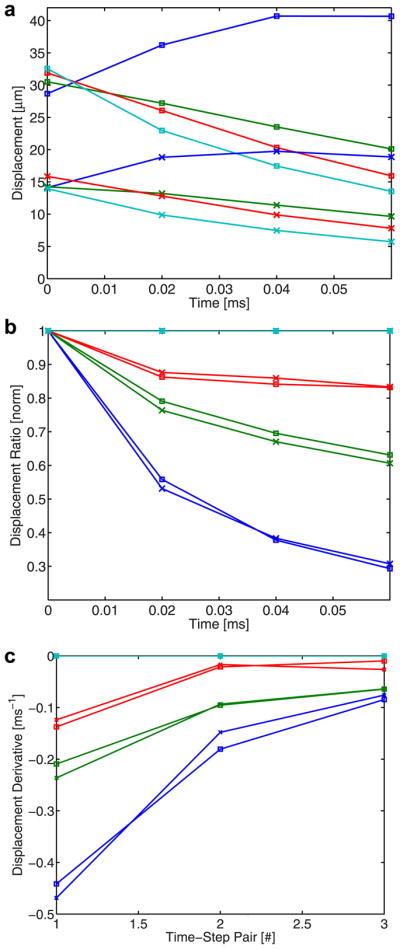
Figure 2a shows the on-axis response based on displacement data averaged about the focus (i.e., one of the beams located in the yellow box in Fig. 1) and displayed for 0.55 ms after the initiation of the ARFI excitation. The DRR method consists of three basic steps (depicted in Fig. 2 [b–d]). First, one of the displacement traces is chosen to be the ratio numerator and (element by element) divided by all of the displacement traces (which serve as denominators). The resulting ratios are then divided by their maximum values to normalize for differences in induced displacement magnitude (e.g., because of intensity variation). In the example given (Fig. 2a), the 18-kPa displacement trace (blue) is divided by all three traces (including itself) and normalized for displacement magnitude variations, resulting in the plot in Fig. 2b. Although the 18-kPa trace was used in this example, in practice any of the displacement traces can serve as the numerator in this ratio.

Fig. 2.

Graphic depiction of the DRR method. In the first plot (a), on-axis displacement resulting from an ARFI excitation in three phantoms (5, 11 and 18 kPa) is shown; time is given in milliseconds after the initiation of the ARFI excitation. In the second plot (b), traces of normalized (to the peak value for each trace) displacement ratios (with the 18-kPa displacement trace as the numerator) are presented. In the third plot (c), traces of finite differences between successive time points (i.e., time-step pairs) is depicted. In the final plot (d), the range of finite difference values for each time-step pair is normalized; the dotted line indicates the expected value.

Fig. 1.

B-mode image (a) of ROI and example of a lateral position vs. time displacement image (b). B-mode image (a) of a portion of the LVFW where the standoff-proximal wall interface can be seen at approximately 12 mm and the distal wall can be seen at approximately 28 mm; the image is of the long axis of the heart, with the base positioned on the right side and the apex on the left side. The red dot indicates the location of the ARFI excitation focus, the yellow box (1.6 × 0.5 mm) indicates the extent/location of the on-axis acquisition region and the pink box (1.6 × 2.1 mm) indicates the extent/location of the off-axis acquisition (i.e., velocimetry) region. Lateral position vs. time displacement image (b) for a fixed-depth kernel, which correlates to the pink box in the B-mode image (a). Presented displacement estimates are obtained by averaging the axial extent of the off-axis region. The Radon sum fit for the shear wave peak trajectory is denoted by the green line, the lateral extent of the off- and on-axis acquisition regions are denoted by the pink and yellow lines, respectively, whereas the lateral location of the ARFI excitation is denoted by a red dot. Note that although the lateral extent of on-axis elements (green and yellow lines) are denoted in the displacement image, the data used in their calculation were obtained from a deeper region of tissue (i.e., about the transmit focus). Red indicates maximum displacement; blue, minimum displacement.

Second, a finite difference (defined as follows) is then calculated for each time-step pair (i.e., temporally adjacent sample points):

$$f(N_t)=\frac{F(t_{n+1})-F(t_n)}{t_{n+1}-t_n},$$ (2)

where N_t is the time-step pair number, F(t) is the normalized displacement ratio at a fixed time and t_n is the time at a specific time step. Note that t_n and t_n+1 is the n-th time-step pair. The finite difference plot for the presented data is shown in Fig. 2c. This step discerns the rate at which a dynamic response in one material is changing (i.e., recovering) relative to this response in another material.

Third, the range of finite difference values for each time-step pair is forced to be a common, arbitrary value (i.e., one). This step is necessary because the recovery rate of the medium (and thus the range of corresponding finite difference values) changes as a function of time after the ARFI excitation (e.g., in Fig. 2c the range changes from approximately 0.6 to 0.2 ms⁻¹ for the first and second time-step pairs, respectively). The relative distribution and ranking of these rates, however, is maintained through time, and thus forcing the range for each time-step pair to an arbitrary value facilitates easier comparison through time and allows for temporal averaging. This final normalization is achieved by first subtracting the lowest finite difference value from all values (for a specific time-step pair) and then by dividing these values by the new maximum for that time-step pair. The result provides a normalized DRR method ranking of shear wave velocity and is presented in Fig. 2d; it can be compared with a similar ranking (using the aforementioned normalization procedure) based on test phantoms’ (to be presented shortly) known shear wave velocities (e.g., 1.25, 1.91, 2.44 m/s becomes 0, 0.55, 1.0) as a control (dotted line). The first three time-step pairs share reasonable agreement to the expected value, and thus their rankings can be averaged. In the example presented, all of the ratios are calculated with the 18-kPa displacement trace as the numerator (i.e., stiffness ranking is achieved by comparing all other traces with the 18-kPa trace). As previously mentioned, the same ranking can be performed with the other two traces as the numerator; these normalized rankings can then be averaged across different time-step pairs and numerator values to improve the robustness of the method. Rankings obtained from different numerators do not yield independent estimates. Given that it is not known a priori which trace(s) will not make a suitable numerator(s) (e.g., a trace with severe motion artifact or poor signal-to-noise ratio), averaging across normalized rankings from all possible numerator values can be performed to mitigate the effect a spurious trace(s) has on the overall ranking.

Experimental system and data processing

Experiments were performed with a SONOLINE Antares^™ ultrasound system using a VF7-3 linear array (Siemens Healthcare, Ultrasound Business Unit, Mountain View, CA, USA) operating at 4.2 MHz (ARFI excitation transmit) and 7.3 MHz (tracking excitation transmit). The array was used to both generate and track ARFI-induced motion. To induce a dynamic response in the myocardium, a 95-μs ARFI pulse, of comparable pulse-average intensity to a conventional B-mode pulse, was transmitted to the region of interest (ROI). Uniaxial tracking (320-μm kernel) was then achieved at specific on-axis and off-axis lateral locations through ultrasonic tracking. Given that the system cannot track all of its available lateral beam locations simultaneously, the employed velocimetry scheme obtains a complete shear wave response of a given lateral extent through superposition of the responses from multiple ARFI excitations delivered to a common ROI. To achieve this, receive beams are tracked at four distinct lateral locations simultaneously through parallel-receive beamforming, which allows for an improved frame rate with a minimal reduction in tracking performance (Dahl et al. 2007; Bouchard et al. 2009a).

To mitigate the effects of physiologic motion, a motion filter was used for all acquisitions. For those sequences involving later-time dynamics (i.e., ARFI imaging and velocimetry), an interpolation-based motion filter was used (Hsu et al. 2009). In short, a quadratic fit is made between pre-ARFI tracking data and post-ARFI data (i.e., when the material is thought to have fully recovered); this fit is then subtracted from the tracked response observed during ARFI-induced dynamics. For the DRR method, which involves early-time dynamics (i.e., <0.5 ms after an ARFI excitation), an extrapolation-based motion filter was used (Giannantonio et al. 2009). In short, a linear fit is performed on pre-ARFI tracking data, and this fit is subtracted from the early-time response experienced during ARFI-induced dynamics.

For the purpose of shear wave velocimetry, the Radon sum transformation shear wave velocimetry method was used (Rouze et al. 2010). In Fig. 1b, displacement data are plotted as a function of lateral position and time after an ARFI excitation. In the image, displacement data are normalized to the maximum value for each lateral position. The red region of the image results from the peak of the shear wave propagating to more distant lateral locations through time. To estimate the velocity of this wave, displacement data are summed along all linear trajectories through a set lateral range (as defined by the pink box in Fig. 1a). The trajectory with the greatest summation is then deemed the best fit (green line) for a shear wave peak’s trajectory.

Validation

Phantom studies

For the first phantom study, both DRR and shear wave velocimetry data were acquired. The ultrasound transducer was fixed above custom-made, Zerdin-based tissue-mimicking phantoms (CIRS, Norfolk, VA, USA), each with ultrasonic attenuation of 0.5 dB/cm/MHz and speed of sound of 1540 m/s. Using the aforementioned Radon sum transformation technique, the shear wave velocities of the four homogeneous phantoms were assessed to determine a gold standard and are: 1.25 ± 0.01, 1.91 ± 0.005, 2.44 ± 0.03 and 2.53 ± 0.02 m/s. From these mean values and using the relationship in eqn (1) (and assuming v =0.5 and ρ =1.0 g/cm³), the Young’s moduli of the phantoms were determined to be: 4.7, 11.0, 17.9 and 19.2 kPa.

The second part of the phantom analysis investigated the impact of variations in ARFI intensity on the DRR method. In this study, two ARFI pulses with different intensities were transmitted in each of the aforementioned phantoms. Because the intensities of these transmit pulses were not measured, they are differentiated by relative terms (i.e., “higher” and “lower” intensity). Continuing with the investigation of ARFI excitation intensity variation, in the third study a phantom with two regions of differing stiffness was analyzed with both ARFI imaging (for comparison) and the DRR method. Data were acquired in a fifth, Zerdine-based tissue-mimicking phantom (CIRS, Inc.) that was heterogeneous in its composition (Fig. 5a), having two adjacent and homogeneous regions of varied stiffness. In this study, a lower-intensity ARFI excitation was transmitted in the more compliant region (4.7 kPa) and a higher-intensity excitation was transmitted in the stiffer region (19.2 kPa). Note that ARFI excitation intensity was changed, for demonstration purposes, only in the aforementioned second and third studies and was kept constant for all other experiments.

Fig. 5.

B-mode (a), ARFI imaging (b) and DRR method plot (c) of an acquisition in a heterogeneous phantom. The B-mode image (a) identifies the two stiffness regions of the phantom; the cyan box indicates the DRR sampling region. In the center plot (b), the ARFI imaging peak displacement result is given; the color bar corresponds to microns of displacement. On the right (c), a DRR method plot obtained from displacement data about the transmit focus is offered. In all depictions, a green line indicating the discrete interface between stiffness regions is shown, whereas lines at the top of each image indicate the relative (higher = yellow; lower = pink) intensity of the ARFI excitation used in each region.

Numerical modeling

Three-dimensional finite element method (FEM) models of the dynamic response of purely elastic media to ARFI excitations were used as a numerical comparison with results from the first phantom study. Numerical modeling permits the analysis of the full dynamic response—including early-time dynamics—absent of ultrasound-based tracking bias or noise (Palmeri et al. 2006a,b). The model used a mesh of 750,000 eight-noded, linear cubic elements with 0.1-mm node spacing and was created in three dimensions (lateral/elevational: 0.5 mm; depth 3.0 mm) using quarter-symmetry (about the transducer’s axis of symmetry) boundary conditions. Degrees of freedom for the symmetry faces were set for their appropriate symmetry conditions, the other “outer” faces were unconstrained and the bottom and top boundaries were fully constrained. The material was modeled as a linear, isotropic, elastic solid with v = 0.499 and ρ = 1.0 g/cm³. Materials were modeled to have Young’s moduli values based on the relationship in eqn (1) and shear wave velocity estimates for the actual phantoms used in experimentation. Simulation of the acoustic intensity pattern associated with the transducer used in the phantom and in vivo experiments was performed using Field II, a linear acoustics modeling software package (Jensen and Svendsen 1992). The radiation force field was applied as point loads to individual nodes in the region of excitation. Forces were directed along the Poynting vector as a function of position in the region of excitation. The dynamic response of the elastic solid was solved through the balance of linear momentum and using LS-DYNA3D (Livermore Software Technology Corp., Livermore, CA, USA), which implemented an explicit, time-domain, integration method (Palmeri et al. 2005).

Animal study protocol

For the in vivo portion of the protocol, two open-chest preparation canine studies, approved by the Institutional Animal Care and Use Committee at Duke University and conforming to the Research Animal Use Guidelines of the American Heart Association, were performed. The mongrel dogs were approximately 20 kg in mass with a heart rate of 67–87 bpm during sequence acquisition. In an effort to mitigate lateral motion, the ultrasound transducer was attached to a vacuum-driven coupling device with an Aquaflex ultrasonically-transparent, 10-mm standoff (Parker Laboratories, Fairfield, NJ, USA) placed between the heart and the transducer; a more detailed explanation of this experimental component can found in Hsu et al. (2009) and Bouchard et al. (2009b). After a left thoracotomy, the pericardium was opened, and the transducer and attached vacuum-coupling device were placed directly on the exposed epicardium; the transducer’s long axis was approximately aligned with the long axis of the heart. The transmit focus was 17.5 mm, which was about 5–6 mm beyond the distal border of the standoff pad. Matched electrocardiogram and ARFI excitation trigger traces were obtained off-line to determine the temporal registration between sequence acquisition and the cardiac cycle. Twenty (on-axis and off-axis) acquisitions (20 ms in length) were obtained at even intervals through nearly two complete heartbeats. For each acquisition, data were acquired for ARFI imaging, velocimetry and DRR method analysis. Presented DRR method plots were obtained by averaging all twenty rankings that resulted from the use of each displacement trace (i.e., one obtained during each acquisition) as the numerator in DRR analysis.

RESULTS

Simulation and phantom

The first part of the simulation and phantom data focuses on the DRR method’s ability to rank shear wave velocities in elastic media of four distinct stiffnesses. In Fig. 3, simulation (a) and phantom (b) results for the DRR method are compared with expected values across the first three time-step pairs. For each time-step pair, the presented ranking is generated from averaging four normalized rankings obtained by having each displacement trace for a specific modulus serve as the numerator in the displacement ratio. The full range of this averaged ranking is then forced to one (using the normalization approach described in Methods); ranking of the known stiffnesses of the four media is then converted to this same range for the purpose of comparison (depicted by horizontal lines in Fig. 3 [a, b]) and error determination (i.e., known stiffness rank distribution vs. DRR method estimate). For the simulation results (a), the mean ± SD (across the three time-step pairs) absolute error (based on normalized, i.e., 0–1, DRR values) for the 11-kPa phantom (green) is 0.05 ±0.03 for both the 0-mm (square) and 0.2-mm (asterisk) receive-beam offsets; for the 18-kPa phantom (red), they are 0.01 ± 0.002 and 0.02 ± 0.02 for 0-mm and 0.2-mm offsets, respectively. For the phantom results (b), the mean ± SD absolute errors for the 11-kPa phantom (green) are 0.14 ± 0.03 and 0.18 ± 0.09 for 0-mm and 0.2-mm offsets, respectively; for the 18-kPa phantom (red), they are 0.11 ± 0.08 and 0.07 ± 0.06 for 0-mm and 0.2-mm offsets, respectively; for the 19-kPa phantom, it is 0.04 ± 0.08 for the 0-mm offset. All other unmentioned error values are zero, which reflects these data’s use as normalization values. The average (across time-step pairs and both beam offsets) of the simulation and phantom DRR method values were then taken to establish an overall shear wave velocity ranking for the four phantoms. The normalized average rankings for the simulation (square) and phantom (asterisk) results were plotted (Fig. 3c) as a function of shear wave velocity in the respective media. The cyan line depicts the expected DRR method ranking based on the known shear wave velocity of a medium. For the simulation results (square), the absolute errors for the 11-kPa and 18-kPa media are 0.05 and 0.02, respectively; for the phantom results, the absolute error for both media is 0.05.

Fig. 3.

DRR method results from simulation (a) and phantom (b) data and a comparison of these results with expected values (c). In the first plot, DRR rankings based on simulation data (a) for phantoms of four different stiffnesses (blue =5 kPa; green = 11 kPa; red = 18 kPa; cyan = 19 kPa) are offered. DRR rankings are determined for three time-step pairs and for two beam locations (square = 0 mm offset; asterisk = 0.2 mm offset). In the second plot, DRR rankings are presented for phantom data (b) with comparable experimental parameters to the simulation configuration. In both plots, horizontal lines indicate expected values. In the final plot (c), a comparison of the average (between three time-step pairs for two lateral locations) simulation-based (square) and phantom- based (asterisk) DRR rankings for each material stiffness is offered. Ranking values are plotted as a function of a material’s shear wave velocity; the cyan line indicates expected DRR rank values.

The second phantom study investigates the DRR method’s insensitivity to ARFI excitation intensity fluctuation. On average, the peak displacement induced by the higher-intensity excitation is 2.1 times greater than the displacement induced by the lower intensity excitation for all of the phantoms presented (Fig. 4a). The other two axes offer the normalized displacement ratio plot (b), with the 19-kPa displacement trace as the numerator, and finite difference plot (c) of these ratios. For each phantom stiffness, displacement ratio traces are similar between the higher (square) and lower (‘x’) intensity data. Likewise, finite differences are similar for matched traces (i.e., same stiffness modulus). Finite difference values begin to converge with increased time-step pair number.

Fig. 4.

On-axis displacement profiles (a), normalized displacement ratio profiles (b) and finite difference plot (c) resulting from ARFI excitations of two different intensities. In the displacement plot (a), displacement profiles generated in phantoms of four stiffnesses (same color coding as Fig. 3) from higher (square) and lower (‘x’) intensity ARFI excitations are depicted. In the three stiffer phantoms, displacement tracking begins after the peak in ARFI-induced displacement has already occurred. In the ratio plot (b), normalized ratio traces, with the 19-kPa displacement profiles (cyan) serving as the numerator, are presented.

In the third phantom study, the effect of variations in ARFI excitation intensity on the DRR method and ARFI imaging is investigated in a heterogeneous phantom (Fig. 5a). Figure 5b presents ARFI imaging data at a fixed time (intended to be the approximate point of maximum displacement) after the excitation. In the 19.2-kPa region, the mean ± SD of the displacement about the focus (i.e., same depth range as the yellow box in Fig. 1a) is 15.4 ± 2.2 μm; in the 4.7-kPa region, mean displacement about the focus is 13.5 ± 3.4 μm. Given the use of the higher intensity excitation, peak displacement is greater in the stiffer region than that achieved in the more compliant region, which was sampled with a lower intensity excitation. If the DRR method is applied to these same regions, the plot in Fig. 5c results. In establishing this averaged DRR ranking, the displacement traces of 23 sampled lateral locations were used as ratio numerators, and these rankings were averaged and normalized to establish an overall ranking (which is shown). The mean ± SD DRR value for the stiffer (i.e., 19.2 kPa) region (excluding the transition point nearest the green line) is 0.78 ± 0.14. For the more compliant region (again, excluding the transition point), the mean DRR value is 0.09 ± 0.09.

Animal study

Figure 6 presents results from an experimental trial during the first in vivo canine study. The upper portion of the figure offers the electrocardiogram trace during acquisition, with the 20 sample periods denoted in red. Directly below the sample numbers are images of the data used for shear wave velocity estimation. The dark red portion of each image indicates the peak of the shear wave. In most cases, the Radon sum fit appears to follow a clearly delineated and fairly linear red contour (which is the trajectory of the shear wave peak through time). Instances when the fit was less reliable include times of increased motion and seemingly nonlinear peak trajectory. In the cases of acquisitions #4 and #9, aberrant displacement peaks can be observed away from the axis of the Radon sum fit. There are also cases where the shear wave peak data (red) are discontinuous and sudden shifts of the peak (in time) can be observed between adjacent lateral locations. In most cases where discontinuities exist, peak data are continuous for groups of four lateral locations, and a sudden shift (in time) is observed between adjacent four-beam groups; this discontinuity effect is especially pronounced in acquisitions #1 and #16. The lower-middle portion of the figure shows the estimated shear wave speed and DRR values through the cardiac cycle. In the shear wave velocity data, the highest speeds come during end-diastole/systole and the lowest velocities are observed during mid-diastole. Shear wave velocities range from 1.97–0.81 m/s, for a systolic-to-diastolic shear wave velocity ratio of 2.4. The shear wave velocity trace (blue) and DRR method trace (green) present trends with similar cyclic variation. In the ARFI imaging data (bottom plot in Fig. 6), despite the fairly stable and similar contour of the waveforms for all three plot-time points (i.e., the time after ARFI excitation at which the displacement estimate is made), the ratio of maximum to minimum displacement varies among the three traces. If the ratio of the maximum to minimum (positive) displacement for each plot-time point is taken, ratios of 6.1, 10.0 and 74.5 result for the 0.2, 0.7 and 1.1 ms plot-time points, respectively. In addition, it is important to note that negative displacement estimates are observed during mid-systole for the 0.7- and 1.1-ms time points. The LVFW wall thickness ranged from approximately 18 (diastole) to 27 (systole) mm through the cardiac cycle.

Fig. 6.

Electrocardiogram trace (upper), normalized shear wave data (upper middle), shear wave velocity and DRR method plots (lower middle) and ARFI-imaging displacement plots (lower) from an experimental trial during the first in vivo cardiac study. In the upper plot, the electrocardiogram trace through the acquisition period is given in cyan, with the time and duration of the 20 independent ARF-based acquisitions denoted with the overlaid red trace and accompanying acquisition number. In the lower-middle row of the figure, raw data (i.e., lateral position vs. time images) used to determine shear wave velocity estimates for each of the corresponding 20 acquisition regions given directly above are presented; the Radon sum fit for each plot is given by the green line. In each image, lateral position is the ordinate and time is the abscissa. In the lower-middle plot, shear wave velocity estimates (blue) and DRR method rankings (green) are given throughout the cardiac cycle, with dots corresponding to the sample locations denoted directly above as red in the electrocardiogram trace. In the lower plot, average ARFI imaging displacement about the focus is given for three different plot-time points.

Figure 7 presents an experimental trial from the second in vivo canine study. Much like the first dataset (Fig. 6), a cyclic variation is observed in both the shear wave velocity and DRR values. The range of shear wave velocities for this data set is between 1.91 and 0.78 m/s, which establishes a systolic-to-diastolic velocity ratio of 2.4. Note there is a significant discontinuity in the shear wave peak (i.e., red region) in acquisition #13. In the case of ARFI imaging (bottom plot in Fig. 7), if the ratio of the maximum to minimum (positive) displacement for each plot-time point is taken, ratios of 5.1, 25.2 and 16.5 result for the 0.2, 0.7 and 1.1 ms plot-time points, respectively.

Fig. 7.

Electrocardiogram trace (upper) and shear wave velocity and DRR method plots (lower) from the second in vivo cardiac study. Conventions are the same as those used in Fig. 6.

Table 1 details the temporal and spatial sampling windows required for each acquisition scheme implemented during both canine studies. The DRR method offers an 97% reduction in sampling time over velocimetry and ARFI imaging offers a 95% reduction in spatial kernel size over velocimetry. Note that the sampling time required for velocimetry is not the fundamental minimum possible for the Radon sum transformation method. If the acquisition system were able to simultaneously track the response of a single excitation at all desired beam locations, this acquisition time would be similar—albeit still greater—than that required for ARFI imaging; the value denoted with the asterisk indicates this time. The full width at half-maximum beam-width was used to calculate the lateral extent of a single beam while the displacement estimation kernel was included in the overall axial extent of the presented sampling windows.

Table 1.

Comparison of acquisition temporal and spatial windows

Method	Temporal (ms)	Spatial (mm2)
Velocimetry	23.2 (5.8*)	3.2
ARFI imaging	4.0	0.2
DRR method	0.8	0.7

Time required for fully parallelized acquisition.

DISCUSSION

Cyclic variation was observed in the metrics of all three methods, which suggests a cyclic variation in stiffness through the cardiac cycle. The general shapes of the velocimetry and DRR data were similar to each other and to the inverse of the ARFI imaging data. Thus, the DRR method appears to offer a novel, force-magnitude–insensitive technique of assessing stiffness variations with a small (temporal/spatial) sampling kernel. In addition, the study demonstrated that it is possible to track shear waves through the cardiac cycle using the Radon sum shear wave velocimetry technique, which yielded velocity estimates ranging from 0.76–2.09 m/s.

The benefits of the DRR method include the use of a small sampling kernel in space and time as well as relative independence on ARFI excitation intensity. In this study, the spatial kernel used for the DRR method acquisition was 1.6 (axial) × 0.5 (lateral) mm², whereas the kernel size needed for the Radon sum shear wave velocimetry method was larger, at 1.6 × 2.1 mm². The temporal sampling window required for the DRR method decreased by 97% over that required by velocimetry. This reduction, however, would be less substantial if the full shear wave response were acquired at each receive-beam location simultaneously, as is the case with supersonic shear imaging (Tanter et al. 2008). ARFI imaging bested both acquisition methods in regard to spatial sampling, using a kernel of only 1.6 × 0.1 mm². In addition, the DRR method appears to be insensitive to fluctuations in ARFI excitation intensity; such an attribute could be useful in situations with spatially or temporally varying ARF generation.

Despite these benefits, however, the DRR method also suffers from significant limitations. Because a finite difference is taken, noise can be detrimental to this technique, causing unreliable estimates of the displacement ratio’s rate of change. To mitigate this effect, reasonably large spatial kernels (through depth) are used in an attempt to yield a more robust displacement estimate. A desire to obtain a change in displacement (between two time points) that is above the displacement estimation noise floor requires adequate temporal sampling, which would provide an interval long enough between time-step pairs to ensure a measurable change in displacement. Yet, this sampling rate must also be high enough to ensure capture of the early portion of the dynamic response. In the case of stiffer media, this relaxation occurs very quickly after ARFI excitation transmission. Thus, it might only be possible to track the response a few times before tissue recovery has progressed beyond use for the DRR method. In the case of stiffer tissues, a significant portion of the recovery occurs before the first displacement estimate, which renders the DRR method unusable.

Another limitation is that the DRR method assumes a linear, elastic, isotropic medium, which is an accurate assumption for the phantoms used in the method’s validation but might not be entirely valid in other circumstances. A primary factor influencing the displacement rate of a purely elastic medium in response to an impulsive perturbation is the medium’s recovery rate, which is driven by its intrinsic shear wave velocity. It requires such a wave to transport the strain energy (resulting from the localized perturbation) away from the ROI; this redistribution of energy leads to a natural reduction in the system’s total potential energy and a mechanical “recovery” at the perturbation site. If other factors influence the observed response (e.g., physiologic motion artifact or material viscosity), such an indirect approach to discern shear wave velocity or stiffness information could be rendered inaccurate. In addition, because the output of the DRR method is based on relative comparisons of all sampled dynamic responses, this ranking can become unstable if data are included from sampling events for which the majority of the ARFI-induced dynamic response has already occurred (e.g., as can be the case in stiffer materials). Thus, if motion-filtered displacement data do not include a (relatively) monotonic decrease to a (relative) steady state (i.e., the fully recovered state) during the sampling period (i.e., a few milliseconds), then it is likely the ARFI-induced response has already occurred and the data should be excluded from DRR analysis.

In regard to the observed shear wave velocities (0.76 to 2.09 m/s), which were used as the gold standard in the method comparison, it must be noted that their range is generally below that measured by Kanai (2005) (2 to 4.5 m/s, during early diastole) and Rump et al. (2007) (2.5 ± 0.4 m/s, throughout cardiac cycle) for mechanical wave velocities through the IVS. In addition, Rump et al. (2007) did not observe significant cyclic variation in their velocity data. Two possible sources of the discrepancy between the results presented herein and those included in the aforementioned studies are the use of a varied ROI site (LVFW vs. IVS) and excitation mechanism. Different excitation mechanisms could excite different wave modes (e.g., shear vs. Lamb wave) that would not necessarily travel at the same speed. In addition, different excitation mechanisms can excite waves with varied frequency content, which, as a result of dispersion, can lead to varied wave speeds (Tanter et al. 2008). For the sake of elasticity imaging, the accurate conversion of the shear wave velocity values to absolute stiffness metrics is not always trivial. If one assumes a shear wave is generated and that it is traveling through a linear, elastic, isotropic environment, then eqn (1) can be used to estimate a material stiffness in said medium. Likewise, if these assumptions are made for the cardiac study, a systolic-to-diastolic stiffness ratio of 5.8 can be estimated from the shear wave velocity data presented herein. With the composition of the LVFW violating the major assumptions (i.e., linear, elastic, isotropic) of this basic model, it is, however, unlikely that such a straightforward approach will be possible for the purposes of estimating an exact stiffness ratio. Although the investigation of a more robust model is outside the scope of this paper, the basic result (i.e., increased stiffness during systole when compared with diastole), is noteworthy.

The effect, if any, that the vacuum-coupling device has on observed myocardial elasticity is not known and must be investigated in future experimentation. In addition, epicardial imaging, as performed for all of the in vivo studies presented herein, clearly will not suffice as a means for clinical application of the DRR method. Instead, any viable approach likely must be based on intra-cardiac, transthoracic or transesophageal imaging. An intracardiac implementation would give direct, local access to the heart’s chambers, which facilitates unencumbered delivery of ARF to the intended ROI. Although there are inherent benefits to a catheter-based approach, the invasiveness of such procedures could limit their use. Thus, a transthoracic or transesophageal implementation promises a much easier clinical application, despite the significant hindrances (e.g., generating appreciable ARF at the ROI) that must first be overcome. The use of a phased-array transducer—as opposed to the linear-array device used herein—will likely be necessary given the limited acoustic window afforded by these imaging methods.

CONCLUSION

The DRR method offers an intensity-independent technique of assessing relative changes in stiffness with a small temporal and spatial sampling window. Limitations to its implementation, however, include its vulnerability to displacement estimation noise, inability to operate in tissues of higher stiffness and inability to offer a quantitative metric. In addition, the Radon sum transformation velocimetry technique, which was used as a gold standard, was able to reliably track shear waves in the myocardium throughout the entire cardiac cycle, with velocities from 0.76 (diastole) to 1.97 (systole) m/s. If a basic elasticity model is assumed, this cyclic variation in wave speed suggests a systolic-to-diastolic stiffness ratio of 5.8. Although the DRR method does not offer quantitative metrics, it does predict a similar cyclic variation in myocardial stiffness to that offered by velocimetry data while being insensitive to variations in ARF and offering improved temporal/spatial sampling.

UNCITED REFERENCES

Byram et al., 2010; Connelly et al., 1991; Jegger et al., 2007; Kundu, 2004; McVeigh, 1996; Mügge et al., 1991; Nyborg,; Pernot et al., 2007; Pinton et al., 2006; Skowronski et al., 1991; Viktorov, 1967; Weisse et al., 1970.

References

- Amundsen BH, Helle-Valle T, Edvardsen T, Torp H, Crosby J, Lyseggen E, Stoylen A, Ihlen H, Lima J, Smiseth O, Slordahl S. Noninvasive myocardial strain measurement by speckle tracking echocardiography: Validation against sonomicrometry and tagged magnetic resonance imaging. J Am Coll Cardiol. 2006;47:789–793. doi: 10.1016/j.jacc.2005.10.040. [DOI] [PubMed] [Google Scholar]
- Behler R, Nichols T, Zhu H, Merricks E, Gallippi C. ARFI imaging for noninvasive material characterization of atherosclerosis part ii: Toward in vivo characterization. Ultrasound Med Biol. 2009;35:278–295. doi: 10.1016/j.ultrasmedbio.2008.08.015. [DOI] [PMC free article] [PubMed] [Google Scholar]
- Bercoff J, Tanter M, Fink M. Supersonic shear imaging: A new technique for soft tissue elasticity mapping. IEEE Trans Ultrason Ferroelectr Freq Control. 2004;51:396–409. doi: 10.1109/tuffc.2004.1295425. [DOI] [PubMed] [Google Scholar]
- Bishop J, Poole G, Plewes D. Magnetic resonance imaging of shear wave propagation in excised tissue. J Magn Reson Imaging. 1998;8:1257–1265. doi: 10.1002/jmri.1880080613. [DOI] [PubMed] [Google Scholar]
- Bouchard RR, Dahl JJ, Hsu SJ, Palmeri ML, Trahey GE. Image quality, tissue heating, and frame rate trade-offs in acoustic radiation force impulse imaging. IEEE Trans Ultrason Ferroelectr Freq Control. 2009a;56:63–76. doi: 10.1109/TUFFC.2009.1006. [DOI] [PMC free article] [PubMed] [Google Scholar]
- Bouchard RR, Hsu SJ, Wolf PD, Trahey GE. In vivo cardiac, acoustic-radiation-force-driven, shear wave velocimetry. Ultrasonic Imaging. 2009b;31:201–213. doi: 10.1177/016173460903100305. [DOI] [PMC free article] [PubMed] [Google Scholar]
- Burkhoff D, Mirsky I, Suga H. Assessment of systolic and diastolic ventricular properties via pressure-volume analysis: A guide for clinical, translational, and basic researchers. Am J Physiol Heart Circ Physiol. 2005;289:501–512. doi: 10.1152/ajpheart.00138.2005. [DOI] [PubMed] [Google Scholar]
- Byram B, Holley G, Giannantonio D, Trahey G. 3-d phantom and in vivo cardiac speckle tracking using a matrix array and raw echo data. IEEE Trans Ultrason Ferroelectr Freq Control. 2010;57:839–854. doi: 10.1109/TUFFC.2010.1489. [DOI] [PMC free article] [PubMed] [Google Scholar]
- Connelly C, McLaughlin R, Vogel W, Apstein C. Reversible and irreversible elongation of ischemic, infarcted, and healed myocardium in response to increases in preload and afterload. Circulation. 1991;84:387–399. doi: 10.1161/01.cir.84.1.387. [DOI] [PubMed] [Google Scholar]
- Dahl J, Pinton G, Palmeri M, Agrawal V, Nightingale K, Trahey G. A parallel tracking method for acoustic radiation force impulse imaging. IEEE Trans Ultrason Ferroelectr Freq Control. 2007;54:301–312. doi: 10.1109/tuffc.2007.244. [DOI] [PMC free article] [PubMed] [Google Scholar]
- D’hooge J, Konofagou E, Jamal F, Heimdal A, Barrios L, Bijnens B, Thoen J, Van de Werf F, Sutherland G, Suetens P. Two-dimensional ultrasonic strain rate measurement of the human heart in vivo. IEEE Trans Ultrason Ferroelectr Freq Control. 2002;49:281–286. doi: 10.1109/58.985712. [DOI] [PubMed] [Google Scholar]
- Fatemi M, Greenleaf JF. Topics in applied physics. Berlin/Heidelberg: Springer; 2002. [Google Scholar]
- Giannantonio G, Byram B, Trahey G. Comparison of alternate physiological motion filters for in vivo cardiac ARFI. 8th International Conference on the Ultrasonic Measurement and Imaging of Tissue Elasticity; 2009. [Google Scholar]
- Gorcsan J, Gulati V, Mandarino W, Katz W. Color-coded measures of myocardial velocity throughout the cardiac cycle by tissue Doppler imaging to quantify regional left ventricular function. Am Heart J. 1996;131:1203–1213. doi: 10.1016/s0002-8703(96)90097-6. [DOI] [PubMed] [Google Scholar]
- Holmes J, Borg T, Covell J. Structure and mechanics of healing myocar-dial infarcts. Annu Rev Biomed Eng. 2005;7:223–253. doi: 10.1146/annurev.bioeng.7.060804.100453. [DOI] [PubMed] [Google Scholar]
- Hsu S, Bouchard R, Dumont D, Wolf P, Trahey G. In vivo assessment of myocardial stiffness with acoustic radiation force impulse imaging. Ultrasound Med Biol. 2007;33:1706–1719. doi: 10.1016/j.ultrasmedbio.2007.05.009. [DOI] [PMC free article] [PubMed] [Google Scholar]
- Hsu SJ, Bouchard RR, Dumont DM, Ong CW, Wolf PD, Trahey GE. Novel acoustic radiation force impulse imaging methods for visualization of rapidly moving tissue. Ultrason Imaging. 2009;31:183–200. doi: 10.1177/016173460903100304. [DOI] [PMC free article] [PubMed] [Google Scholar]
- Jegger D, Mallik AS, Nasratullah M, Jeanrenaud X, da Silva R, Tevaearai H, von Segesser LK, Stergiopulos N. The effect of a myocardial infarction on the normalized time-varying elastance curve. J Appl Physiol. 2007;102:1123–1129. doi: 10.1152/japplphysiol.00976.2006. [DOI] [PubMed] [Google Scholar]
- Jensen J, Svendsen N. Calculation of pressure fields from arbitrarily shaped, apodized, and excited ultrasound transducers. IEEE Trans Ultrason Ferroelectr Freq Control. 1992;39:262–267. doi: 10.1109/58.139123. [DOI] [PubMed] [Google Scholar]
- Kanai H. Propagation of spontaneously actuated pulsive vibration in human heart wall and in vivo viscoelasticity estimation. IEEE Trans Ultrason Ferroelectr Freq Control. 2005;52:1931–1942. doi: 10.1109/tuffc.2005.1561662. [DOI] [PubMed] [Google Scholar]
- Kundu T. Ultrasonic nondestructive evaluation: Engineering and biological characterization. Boca Raton: CRC Press; 2004. [Google Scholar]
- Lai W, Rubin D, Krempl E. Introduction of continuum mechanics. Oxford: Pergamon Press; 1993. [Google Scholar]
- Lloyd-Jones D, Adams RJ, Brown TM, Carnethon M, Dai S, De Simone G, Ferguson T, Ford E, Furie K, Gillespie C, Go A, Greenlund K, Haase N, Hailpern S, Ho P, Howard V, Kissela B, Kittner S, Lackland D, Lisabeth L, Marelli A, McDermott M, Meigs J, Mozaffarian D, Mussolino M, Nichol G, Roger V, Rosamond W, Sacco R, Sorlie P, Stafford R, Thom T, Wasserthiel-Smoller S, Wong N, Wylie-Rosett J American Heart Association Statistics Committee and Stroke Statistics Subcommittee. Heart disease and stroke statistics–2010 update: A report from the American Heart Association. Circulation. 2010;121:46. doi: 10.1161/CIRCULATIONAHA.109.192667. [DOI] [PubMed] [Google Scholar]
- Lyons M, Parker K. Absorption and attenuation in soft tissue ii—experimental results. IEEE Trans Ultrason Ferroelectr Freq Control. 1988;35:511–521. doi: 10.1109/58.4189. [DOI] [PubMed] [Google Scholar]
- Madaras EI, Barzilai B, Perez JE, Sobel BE, Miller JG. Changes in myocardial backscatter throughout the cardiac cycle. Ultrason Imaging. 1983;5:229–239. doi: 10.1177/016173468300500303. [DOI] [PubMed] [Google Scholar]
- McVeigh ER. MRI of myocardial function: Motion tracking techniques. Magn Reson Imaging. 1996;14:137–150. doi: 10.1016/0730-725x(95)02009-i. [DOI] [PubMed] [Google Scholar]
- Melodelima D, Bamber J, Duck F, Shipley J, Xu L. Elastography for breast cancer diagnosis using radiation force: System development and performance evaluation. Ultrasound Med Biol. 2006;32:387–396. doi: 10.1016/j.ultrasmedbio.2005.12.003. [DOI] [PubMed] [Google Scholar]
- Mirsky I, Tajimi T, Peterson KL. The development of the entire end-systolic pressure-volume and ejection fraction-afterload relations: A new concept of systolic myocardial stiffness. Circulation. 1987;76:343–356. doi: 10.1161/01.cir.76.2.343. [DOI] [PubMed] [Google Scholar]
- Mügge A, Daniel WG, Haverich A, Lichtlen PR. Diagnosis of noninfective cardiac mass lesions by two-dimensional echocardiography. Comparison of the transthoracic and transesophageal approaches Circulation. 1991;83:70–78. doi: 10.1161/01.cir.83.1.70. [DOI] [PubMed] [Google Scholar]
- Muthupillai R, Lomas DJ, Rossman PJ, Greenleaf JF, Manduca A, Ehman RL. Magnetic resonance elastography by direct visualization of propagating acoustic strain waves. Science. 1995;269:1854–1857. doi: 10.1126/science.7569924. [DOI] [PubMed] [Google Scholar]
- Nightingale K, McAleavey S, Trahey G. Shear-wave generation using acoustic radiation force: In vivo and ex vivo results. Ultrasound Med Biol. 2003;29:1715–1723. doi: 10.1016/j.ultrasmedbio.2003.08.008. [DOI] [PubMed] [Google Scholar]
- Nightingale K, Palmeri M, Nightingale R, Trahey G. On the feasibility of remote palpation using acoustic radiation force. J Acoust Soc Am. 2001;110:625–634. doi: 10.1121/1.1378344. [DOI] [PubMed] [Google Scholar]
- Nyborg W. Acoustic streaming. In: Mason W, editor. Physical acoustics. IIB. New York: Academic Press Inc; pp. 265–331. *** [Google Scholar]
- Palmeri M, McAleavey S, Fong K, Trahey G, Nightingale K. Dynamic mechanical response of elastic spherical inclusions to impulsive acoustic radiation force excitation. IEEE Trans Ultrason Ferroelectr Freq Control. 2006a;53:2065–2079. doi: 10.1109/tuffc.2006.146. [DOI] [PMC free article] [PubMed] [Google Scholar]
- Palmeri M, McAleavey S, Trahey G, Nightingale K. Ultrasonic tracking of acoustic radiation force-induced displacements in homogeneous media. IEEE Trans Ultrason Ferroelectr Freq Control. 2006b;53:1300–1313. doi: 10.1109/tuffc.2006.1665078. [DOI] [PMC free article] [PubMed] [Google Scholar]
- Palmeri M, Sharma A, Bouchard R, Nightingale R, Nightingale K. A finite-element method model of soft tissue response to impulsive acoustic radiation force. IEEE Trans Ultrason Ferroelectr Freq Control. 2005;52:1699–1712. doi: 10.1109/tuffc.2005.1561624. [DOI] [PMC free article] [PubMed] [Google Scholar]
- Palmeri M, Wang M, Dahl J, Frinkley K, Nightingale K. Quantifying hepatic shear modulus in vivo using acoustic radiation force. Ultrasound Med Biol. 2008;34:546–558. doi: 10.1016/j.ultrasmedbio.2007.10.009. [DOI] [PMC free article] [PubMed] [Google Scholar]
- Pernot M, Fujikura K, Fung-Kee-Fung S, Konofagou E. ECG-gated, mechanical and electromechanical wave imaging of cardiovascular tissues in vivo. Ultrasound Med Biol. 2007;33:1075–1085. doi: 10.1016/j.ultrasmedbio.2007.02.003. [DOI] [PubMed] [Google Scholar]
- Pinton GF, Dahl JJ, Trahey GE. Rapid tracking of small displacements with ultrasound. IEEE Trans Ultrason Ferroelectr Freq Control. 2006;53:1103–1117. doi: 10.1109/tuffc.2006.1642509. [DOI] [PubMed] [Google Scholar]
- Pislaru C, Bruce CJ, Anagnostopoulos PC, Allen JL, Seward JB, Pellikka PA, Ritman EL, Greenleaf JF. Ultrasound strain imaging of altered myocardial stiffness: Stunned versus infarcted reperfused myocardium. Circulation. 2004;109:2905–2910. doi: 10.1161/01.CIR.0000129311.73402.EF. [DOI] [PubMed] [Google Scholar]
- Rouze N, Wang MH, Palmeri M, Nightingale K. Robust estimation of time-of-flight shear wave speed using a radon sum transformation. IEEE Trans Ultrason Ferroelectr Freq Control. 2010;57:2662–2670. doi: 10.1109/TUFFC.2010.1740. [DOI] [PMC free article] [PubMed] [Google Scholar]
- Rump J, Klatt D, Braun J, Warmuth C, Sack I. Fractional encoding of harmonic motions in MR elastography. Magn Reson Med. 2007;57:388–395. doi: 10.1002/mrm.21152. [DOI] [PubMed] [Google Scholar]
- Sack I, Rump J, Elgeti T, Samani A, Braun J. MR elastography of the human heart: Noninvasive assessment of myocardial elasticity changes by shear wave amplitude variations. Magn Reson Med. 2009;61:668–677. doi: 10.1002/mrm.21878. [DOI] [PubMed] [Google Scholar]
- Sarvazyan A, Rudenko O, Swanson S, Fowlkes J, Emelianov S. Shear wave elasticity imaging: A new ultrasonic technology of medical diagnostics. Ultrasound Med Biol. 1998;24:1419–1435. doi: 10.1016/s0301-5629(98)00110-0. [DOI] [PubMed] [Google Scholar]
- Skowronski E, Epstein M, Ota D, Hoagland P, Gordon J, Adamson R, McDaniel M, Peterson K, Smith S, Jaski B. Right and left ventricular function after cardiac transplantation. Changes during and after rejection. Circulation. 1991;84:2409–2417. doi: 10.1161/01.cir.84.6.2409. [DOI] [PubMed] [Google Scholar]
- Tanter M, Bercoff J, Athanasiou A, Deffieux T, Gennisson J, Montaldo G, Muller M, Tardivon A, Fink M. Quantitative assessment of breast lesion viscoelasticity: Initial clinical results using supersonic shear imaging. Ultrasound Med Biol. 2008;34:1373–1386. doi: 10.1016/j.ultrasmedbio.2008.02.002. [DOI] [PubMed] [Google Scholar]
- Torr G. The acoustic radiation force. Am J Phys. 1984;52:402–408. [Google Scholar]
- Vasan RS, Levy D. Defining diastolic heart failure: A call for standardized diagnostic criteria. Circulation. 2000;101:2118–2121. doi: 10.1161/01.cir.101.17.2118. [DOI] [PubMed] [Google Scholar]
- Viktorov I. Rayleigh and Lamb waves: Physical theory and applications. New York: Plenum Press; 1967. [Google Scholar]
- Weisse A, Saffa R, Levinson G, Jacobson W, Regan T. Left ventricular function during the early and late stages of scar formation following experimental myocardial infarction. Am Heart J. 1970;79:370–383. doi: 10.1016/0002-8703(70)90424-2. [DOI] [PubMed] [Google Scholar]
- Westervelt P. The theory of steady forces caused by sound waves. J Acoust Soc Am. 1951;23:312–315. [Google Scholar]
- Zile MR, Baicu CF, Gaasch WH. Diastolic heart failure–abnormalities in active relaxation and passive stiffness of the left ventricle. N Engl J Med. 2004;350:1953–1959. doi: 10.1056/NEJMoa032566. [DOI] [PubMed] [Google Scholar]