Mixed Membership Stochastic Blockmodels

Abstract

Observations consisting of measurements on relationships for pairs of objects arise in many settings, such as protein interaction and gene regulatory networks, collections of author-recipient email, and social networks. Analyzing such data with probabilisic models can be delicate because the simple exchangeability assumptions underlying many boilerplate models no longer hold. In this paper, we describe a latent variable model of such data called the mixed membership stochastic blockmodel. This model extends blockmodels for relational data to ones which capture mixed membership latent relational structure, thus providing an object-specific low-dimensional representation. We develop a general variational inference algorithm for fast approximate posterior inference. We explore applications to social and protein interaction networks.

1 Introduction

Modeling relational information among objects, such as pairwise relations represented as graphs, is becoming an important problem in modern data analysis and machine learning. Many data sets contain interrelated observations. For example, scientific literature connects papers by citation, the Web connects pages by links, and protein-protein interaction data connects proteins by physical interaction records. In these settings, we often wish to infer hidden attributes of the objects from the observed measurements on pairwise properties. For example, we might want to compute a clustering of the web-pages, predict the functions of a protein, or assess the degree of relevance of a scientific abstract to a scholar's query.

Unlike traditional attribute data collected over individual objects, relational data violate the classical independence or exchangeability assumptions that are typically made in machine learning and statistics. In fact, the observations are interdependent by their very nature, and this interdependence necessitates developing special-purpose statistical machinery for analysis.

There is a history of research devoted to this end. One problem that has been heavily studied is that of clustering the objects to uncover a group structure based on the observed patterns of interactions. Standard model-based clustering methods, e.g., mixture models, are not immediately applicable to relational data because they assume that the objects are conditionally independent given their cluster assignments. The latent stochastic blockmodel (Snijders and Nowicki, 1997) represents an adaptation of mixture modeling to dyadic data. In that model, each object belongs to a cluster and the relationships between objects are governed by the corresponding pair of clusters. Via posterior inference on such a model one can identify latent roles that objects possibly play, which govern their relationships with each other. This model originates from the stochastic blockmodel, where the roles of objects are known in advance (Wang and Wong, 1987). A recent extension of this model relaxed the finite-cardinality assumption on the latent clusters, via a nonparametric hierarchical Bayesian formalism based on the Dirichlet process prior (Kemp et al., 2004, 2006).

The latent stochastic blockmodel suffers from a limitation that each object can only belong to one cluster, or in other words, play a single latent role. In real life, it is not uncommon to encounter more intriguing data on entities that are multi-facet. For example, when a protein or a social actor interacts with different partners, different functional or social contexts may apply and thus the protein or the actor may be acting according to different latent roles they can possible play. In this paper, we relax the assumption of single-latent-role for actors, and develop a mixed membership model for relational data. Mixed membership models, such as latent Dirichlet allocation (Blei et al., 2003), have emerged in recent years as a flexible modeling tool for data where the single cluster assumption is violated by the heterogeneity within of a data point. They have been successfully applied in many domains, such as document analysis (Minka and Lafferty, 2002; Blei et al., 2003; Buntine and Jakulin, 2006), surveys (Berkman et al., 1989; Erosheva, 2002), image processing (Li and Perona, 2005), transcriptional regulation (Airoldi et al., 2006b), and population genetics (Pritchard et al., 2000).

The mixed membership model associates each unit of observation with multiple clusters rather than a single cluster, via a membership probability-like vector. The concurrent membership of a data in different clusters can capture its different aspects, such as different underlying topics for words constituting each document. The mixed membership formalism is a particularly natural idea for relational data, where the objects can bear multiple latent roles or cluster-memberships that influence their relationships to others. As we will demonstrate, a mixed membership approach to relational data lets us describe the interaction between objects playing multiple roles. For example, some of a protein's interactions may be governed by one function; other interactions may be governed by another function.

Existing mixed membership models are not appropriate for relational data because they assume that the data are conditionally independent given their latent membership vectors. In relational data, where each object is described by its relationships to others, we would like to assume that the ensemble of mixed membership vectors help govern the relationships of each object. The conditional independence assumptions of modern mixed membership models do not apply.

In this paper, we develop mixed membership models for relational data, develop a fast variational inference algorithm for inference and estimation, and demonstrate the application of our technique to large scale protein interaction networks and social networks. Our model captures the multiple roles that objects exhibit in interaction with others, and the relationships between those roles in determining the observed interaction matrix.

Mixed membership and the latent block structure can be reliably recovered from relational data (Section 4.1). The application to a friendship network among students tests the model on a real data set where a well-defined latent block structure exists (Section 4.2). The application to a protein interaction network tests to what extent our model can reduce the dimensionality of the data, while revealing substantive information about the functionality of proteins that can be used to inform subsequent analyses (Section 4.3).

2 The mixed membership stochastic blockmodel

In this section, we describe the modeling assumptions behind our proposed mixed membership model of relational data. We represent observed relational data as a graph $G=(\mathcal{N},R)$, where R(p, q) maps pairs of nodes to values, i.e., edge weights. In this work, we consider binary matrices, where R(p, q) ∈ {0, 1}. Thus, the data can be thought of as a directed graph.

As a running example, we will reanalyze the monk data of Sampson (1968). Sampson measured a collection of sociometric relations among a group of monks by repeatedly asking questions such as “Do you like X?” or “Do you trust X?” to determine asymmetric social relationships within the group. The questionnaire was repeated at four subsequent epochs. Information about these repeated, asymmetric relations can be collapsed into a square binary table that encodes the directed connections between monks (Breiger et al., 1975). In analyzing this data, the goal is to determine the underlying social groups within the monastary.

In the context of the monastery example, we assume K latent groups over actors, and the observed network is generated according to latent distributions of group-membership for each monk and a matrix of group-group interaction strength. The latent per-monk distributions are specified by simplicial vectors. Each monk is associated with a randomly drawn vector, say ${\overrightarrow{\pi }}_i$ for monk i, where π_i,g denotes the probability of monk i belonging to group g. That is, each monk can simultaneously belong to multiple groups with different degrees of affiliation strength. The probabilities of interactions between different groups are defined by a matrix of Bernoulli rates B_(K×K), where B(g, h) represents the probability of having a link between a monk from group g and a monk from group h.

For each network node (i.e., monk), the indicator vector ${\overrightarrow{z}}_{p\to q}$ denotes the group membership of node p when it is approached by node q and ${\overrightarrow{z}}_{p\leftarrow q}$ denotes the group membership of node q when it is approached by node p ¹. N denotes the number of nodes in the graph, and recall that K denotes the number of distinct groups a node can belong to. Now putting everything together, we have a mixed membership stochastic blockmodel (MMSB), which posits that a graph $G=(\mathcal{N},R)$ is drawn from the following procedure.

• For each node $p\in \mathcal{N}$:

  • Draw a K dimensional mixed membership vector ${\overrightarrow{\pi }}_p$ ∼ Dirichlet $(\overrightarrow{\alpha })$.

• For each pair of nodes $(p,q)\in \mathcal{N}\times \mathcal{N}$:

  • Draw membership indicator for the initiator, ${\overrightarrow{z}}_{p\to q}$ ∼ Multinomial $({\overrightarrow{\pi }}_p)$.

  • Draw membership indicator for the receiver, ${\overrightarrow{z}}_{p\to q}$ ∼ Multinomial $({\overrightarrow{\pi }}_q)$.

  • Sample the value of their interaction, R(p, q) ∼ Bernoulli $({\overrightarrow{z}}_{p\to q}^{\top }B{\overrightarrow{z}}_{p\leftarrow q})$.

This process is illustrated as a graphical model in Figure 1. Note that the group membership of each node is context dependent. That is, each node may assume different membership when interacting to or being interacted by different peers. Statistically, each node is an admixture of group-specific interactions. The two sets of latent group indicators are denoted by $\{{\overrightarrow{z}}_{p\to q}:p,q\in \mathcal{N}\}=:Z_{\to }$ and $\{{\overrightarrow{z}}_{p\leftarrow q}:p,q\in \mathcal{N}\}=:Z_{\leftarrow }$. Also note that the pairs of group memberships that underlie interactions, for example, $({\overrightarrow{z}}_{p\to q},{\overrightarrow{z}}_{p\leftarrow q})$ for R(p, q), need not be equal; this fact is useful for characterizing asymmetric interaction networks. Equality may be enforced when modeling symmetric interactions.

Figure 1.

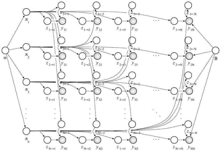
A graphical model of the mixed membership stochastic blockmodel. We did not draw all the arrows out of the block model B for clarity. All the interactions R(p, q) depend on it.

Under the MMSB, the joint probability of the data R and the latent variables $\{{\overrightarrow{\pi }}_{1:N},Z_{\to },Z_{\leftarrow }\}$ can be written in the following factored form,

$$\begin{array}{l}p(R,{\overrightarrow{\pi }}_{1:N},Z_{\to },Z_{\leftarrow }|\overrightarrow{\alpha },B)\\ =\prod _{p,q}P(R(p,q)|{\overrightarrow{z}}_{p\to q},{\overrightarrow{z}}_{p\leftarrow q},B)P({\overrightarrow{z}}_{p\to q}|{\overrightarrow{\pi }}_p)P({\overrightarrow{z}}_{p\leftarrow q}|{\overrightarrow{\pi }}_q)\prod _{p}P({\overrightarrow{\pi }}_p|\overrightarrow{\alpha }).\end{array}$$ (1)

This model easily generalizes to two important cases. (Appendix A develops this intuition more formally.) First, multiple networks among the same actors can be generated by the same latent vectors. This might be useful, for example, for analyzing simultaneously the relational measurements about esteem and disesteem, liking and disliking, positive influence and negative influence, praise and blame, e.g., see Sampson (1968), or those about the collection of 17 relations measured by Bradley (1987). Second, in the MMSB the data generating distribution is a Bernoulli, but B can be a matrix that parameterizes any kind of distribution. For example, technologies for measuring interactions between pairs of proteins such as mass spectrometry (Ho et al., 2002) and tandem affinity purification (Gavin et al., 2002) return a probabilistic assessment about the presence of interactions, thus setting the range of R(p, q) to [0, 1]. This is not the case for the manually curated collection of interactions we analyze in Section 4.3.

The central computational problem for this model is computing the posterior distribution of per-node mixed membership vectors and per-pair roles that generated the data. The membership vectors in particular provide a low dimensional representation of the underlying objects in the matrix of observations, which can be used in the data analysis task at hand. A related problem is parameter estimation, which is to find maximum likelihood estimates of the Dirichlet parameters $\overrightarrow{\alpha }$ and Bernoulli rates B.

For both of these tasks, we need to compute the probability of the observed data. This amounts to marginalizing out the latent variables from Equation 1. This is intractable for even small graphs. In Section 3, we develop a fast variational algorithm to approximate this marginal likelihood for parameter estimation and posterior inference.

2.1 Modeling sparsity

Many real-world networks are sparse, meaning that most pairs of nodes do not have edges connecting them. For many pairs, the absence of an interaction is a result of the rarity of any interaction, rather than an indication that the underlying latent groups of the objects do not tend to interact. In the MMSB, however, all observations (both interactions and non-interactions) contribute equally to our inferences about group memberships and group to group interaction patterns. It is thus useful, in practical applications, to account for sparsity.

We introduce a sparsity parameter ρ ∈ [0, 1] to calibrate the importance of non-interaction. This models how often a non-interaction is due to sparsity rather than carrying information about the group memberships of the nodes. Specifically, instead of drawing an edge directly from the Bernoulli specified above, we downweight it to $\left(1-\rho \right)\cdot {\overrightarrow{z}}_{p\to q}^{\top }B{\overrightarrow{z}}_{p\leftarrow q}$. The probability of having no interaction is thus $1-{\sigma }_{pq}=\left(1-\rho \right)\cdot {\overrightarrow{z}}_{p\to q}^{\top }\left(1-B\right){\overrightarrow{z}}_{p\leftarrow q}+\rho$. (This is equivalent to re-parameterizing the interaction matrix B.) In posterior inference and parameter estimation, a large value of ρ will cause the interactions in the matrix to be weighted more than non-interactions in determining the estimates of $\{\overrightarrow{\alpha },B,{\overrightarrow{\pi }}_{1:N}\}$.

2.2 A case study of the Monastery network via MMSB: crisis in a Cloister

Before turning to the details of posterior inference and parameter estimation, we illustrate the MMSB with an analysis of the monk data described above. In more detail, Sampson (1968) surveyed 18 novice monks in a monastery and asked them to rank the other novices in terms of four sociometric relations: like/dislike, esteem, personal influence, and alignment with the monastic credo. We consider Breiger's collation of Sampson's data (Breiger et al., 1975). The original graph of monk-monk interaction is illustrated in Figure 2 (left).

Figure 2.

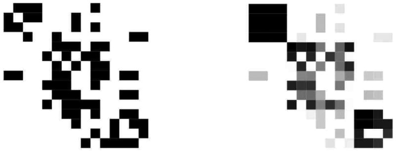
Original matrix of sociometric relations (left), and estimated relations obtained by the model (right).

Sampson spent several months in a monastery in New England, where novices (the monks) were preparing to join a monastic order. Sampson's original analysis was rooted in direct anthropological observations. He strongly suggested the existence of tight factions among the novices: the loyal opposition (whose members joined the monastery first), the young turks (who joined later on), the outcasts (who were not accepted in the two main factions), and the waverers (who did not take sides). The events that took place during Sampson's stay at the monastery supported his observations—members of the young turks resigned after their leaders were expelled over religious differences (John Bosco and Gregory). We shall refer to the labels assigned by Sampson to the novices in the analysis below. For more analyses, we refer to Fienberg et al. (1985), Davis and Carley (2006) and Handcock et al. (2007).

Using the techniques outlined below in Section 3, we fit the monks to MMSB models for different numbers of groups, providing model estimates {α̂, B̂} and posterior mixed membership vectors ${\overrightarrow{\pi }}_n$ for each monk. Here, we use the following approximation to BIC to choose the number of groups in the MMSB:

$$\mathit{\text{BIC}}=2\cdot logp\left(R\right)\approx 2\cdot logp\left(R|\widehat{\overrightarrow{\pi }},\widehat{Z},\widehat{\overrightarrow{\alpha }},\widehat{B}\right)-\left|\overrightarrow{\alpha },B\right|\cdot log\left|R\right|,$$

which selects three groups, where $\left|\overrightarrow{\alpha },B\right|$ is the number of hyper-parameters in the model, and |R| is the number of positive relations observed (Volinsky and Raftery, 2000; Handcock et al., 2007). Note that this is the same number of groups that Sampson identified. We illustrate the fit of model fit via the predicted network in Figure 2 (Right).

The MMSB can provide interesting descriptive statistics about the actors in the observed graph. In Figure 3 we illustrate the the posterior means of the mixed membership scores, $\mathbb{E}\left[\overrightarrow{\pi }|R\right]$, for the 18 monks in the monastery. Note that the monks cluster according to Sampson's classification, with Young Turks, Loyal Opposition, and Outcasts dominating each corner respectively. We can see the central role played by John Bosco and Gregory, who exhibit relations in all three groups, as well as the uncertain affiliations of Ramuald and Victor; Amand's uncertain affiliation, however, is not captured.

Figure 3.

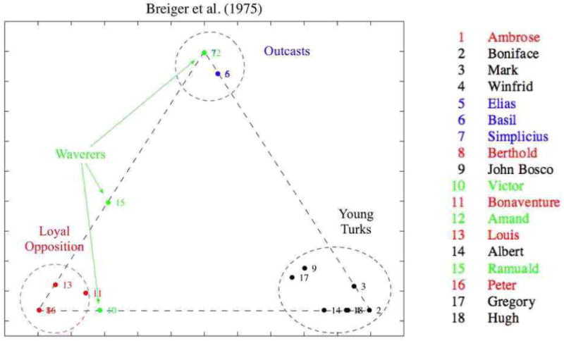
Posterior mixed membership vectors, ${\overrightarrow{\pi }}_{1:18}$, projected in the simplex. The estimates correspond to a model with $B:={\mathbb{I}}_3$, and α̂ = 0.058. Numbered points can be mapped to monks' names using the legend on the right. The colors identify the four factions defined by Sampson's anthropological observations.

Later, we considered six graphs encoding specific relations—positive and negative influence, positive and negative praise, esteem and disesteem—and we performed independent analyses using MMSB. This allowed us to look for signal about the mixed membership of monks to factions that may have been lost in the data set prepared by Breiger et al. (1975) because of averaging. Figure 4 shows the projections in the simplex of the posterior mixed membership vectors for each of the six relations above. For instance, we can see how Victor, Amand, and Ramuald—the three waverers—display mixed membership in terms of positive and negative influence, positive praise, and disesteem. The mixed membership of Amand, in particular, is expressed in terms of these relations, but not in terms of negative praise or esteem. This finding is supported Sampson's anthropological observations, and it suggests that relevant substantive information has been lost when the graphs corresponding to multiple sociometric relations have been collapsed into a single social network (Breiger et al., 1975). Methods for the analysis of multiple sociometric relations are thus to be preferred. In Appendices A and B extend the mixed membership stochastic blockmodel to deal with the case of multivariate relations, and we solve estimation and inference in the general case.

Figure 4.

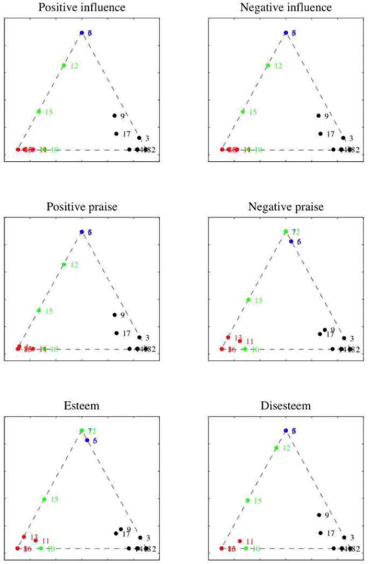
Independent analyses of six graphs encoding the relations: positive and negative influence, positive and negative praise, esteem and disesteem. Posterior mixed membership vectors for each graph, corresponding to models with $B:={\mathbb{I}}_3$, and α̂ via empirical Bayes, are projected in the simplex. (Legend as in Figure 3.)

3 Parameter Estimation and Posterior Inference

In this section, we tackle the two computational problems for the MMSB: posterior inference of the pernode mixed membership vectors and per-pair roles, and parameter estimation of the Dirichlet parameters and Bernoulli rate matrix. We use empirical Bayes to estimate the parameters $\left(\overrightarrow{\alpha },B\right)$, and employ a mean-field approximation scheme (Jordan et al., 1999) for posterior inference.

3.1 Posterior inference

In posterior inference, we would like to compute the posterior distribution of the latent variables given a collection of observations. As for other mixed membership models, this is intractable to compute. The normalizing constant of the posterior is the marginal probability of the data, which requires an intractable integral over the simplicial vectors ${\overrightarrow{\pi }}_p$,

$$p(R|\overrightarrow{\alpha },B)={\mathit{\int }}_{{\overrightarrow{\pi }}_{1:N}}\prod _{p,q}\sum _{z_{p\leftarrow q},z_{p\to q}}P(R(p,q)|{\overrightarrow{z}}_{p\to q},{\overrightarrow{z}}_{p\leftarrow q},B)P({\overrightarrow{z}}_{p\to q}|{\overrightarrow{\pi }}_p)P({\overrightarrow{z}}_{p\leftarrow q}|{\overrightarrow{\pi }}_q)\prod _{p}P({\overrightarrow{\pi }}_p|\overrightarrow{\alpha }).$$ (2)

A number of approxiate inference algorithms for mixed membership models have appeared in recent years, including mean-field variational methods (Blei et al., 2003; Teh et al., 2007), expectation propagation (Minka and Lafferty, 2002), and Monte Carlo Markov chain sampling (MCMC) (Erosheva and Fienberg, 2005; Griffiths and Steyvers, 2004).

We appeal to mean-field variational methods to approximate the posterior of interest. Mean-field variational methods provide a practical deterministic alternative to MCMC. MCMC is not practical for the MMSB due to the large number of latent variables needed to be sampled. The main idea behind variational methods is to posit a simple distribution of the latent variables with free parameters. These parameters are fit to be close in Kullback-Leibler divergence to the true posterior of interest. Good reviews of variational methods method can be found in a number of papers (Jordan et al., 1999; Wainwright and Jordan, 2003; Xing et al., 2003; Bishop et al., 2003)

The log of the marginal probability in Equation 2 can be bound with Jensen's inequality as follows,

$$logp\left(R|\alpha ,B\right)\ge {\mathbb{E}}_q\left[logp\left(R,{\overrightarrow{\pi }}_{1:N},Z_{\to },Z_{\leftarrow }|\alpha ,B\right)\right]-{\mathbb{E}}_q\left[logq\left({\overrightarrow{\pi }}_{1:N},Z_{\to },Z_{\leftarrow }\right)\right],$$ (3)

by introducing a distribution of the latent variables q that depends on a set of free parameters We specify q as the mean-field fully-factorized family,

$$q({\overrightarrow{\pi }}_{1:N},Z_{\to },Z_{\leftarrow }|{\overrightarrow{\gamma }}_{1:N},{\mathrm{\Phi }}_{\to },{\mathrm{\Phi }}_{\leftarrow })=\prod _p{q}_1({\overrightarrow{\pi }}_p|{\overrightarrow{\gamma }}_p)\prod _{p,q}\left(q_2({\overrightarrow{z}}_{p\to q}|{\overrightarrow{\phi }}_{p\to q})q_2({\overrightarrow{z}}_{p\leftarrow q}|{\overrightarrow{\phi }}_{p\leftarrow q})\right),$$ (4)

where q₁ is a Dirichlet, q₂ is a multinomial, and $\{{\overrightarrow{\gamma }}_{1:N},{\mathrm{\Phi }}_{\to },{\mathrm{\Phi }}_{\leftarrow }\}$ are the set of free variational parameters that can be set to tighten the bound.

Tightening the bound with respect to the variational parameters is equivalent to minimizing the KL divergence between q and the true posterior. When all the nodes in the graphical model are conjugate pairs or mixtures of conjugate pairs, we can directly write down a coordinate ascent algorithm for this optimization (Xing et al., 2003; Bishop et al., 2003). The update for the variational multinomial parameters is

$${\widehat{\phi }}_{p\to q,g}\propto e^{{\mathbb{E}}_q\left[log{\pi }_{p,g}\right]}\cdot \prod _h{\left(B{\left(g,h\right)}^{R\left(p,q\right)}\cdot {\left(1-B\left(g,h\right)\right)}^{1-R\left(p,q\right)}\right)}^{{\phi }_{p\leftarrow q,h}}$$ (5)

$${\widehat{\phi }}_{p\leftarrow q,h}\propto e^{{\mathbb{E}}_q\left[log{\pi }_{q,h}\right]}\cdot \prod _g{\left(B{\left(g,h\right)}^{R\left(p,q\right)}\cdot {\left(1-B\left(g,h\right)\right)}^{1-R\left(p,q\right)}\right)}^{{\phi }_{p\to q,g}},$$ (6)

for g, h = 1, …, K. The update for the variational Dirichlet parameters γ_p,k is

$${\widehat{\gamma }}_{p,k}={\alpha }_k+\sum _q{\phi }_{p\to q,k}+\sum _q{\phi }_{p\leftarrow q,k},$$ (7)

for all nodes p = 1,…, N and k = 1,…, K. An analytical expression for ${\mathbb{E}}_q\left[log{\pi }_{q,h}\right]$ is derived in Appendix B.3. The complete coordinate ascent algorithm to perform variational inference is described in Figure 5.

Figure 5.

Top: The two-layered variational inference for $(\overrightarrow{\gamma },{\phi }_{p\to q,g},{\phi }_{p\leftarrow q,h})$ and M = 1. The inner algorithm consists of Step 5. The function f is described in details in the bottom panel. The partial updates in Step 6 for $\overrightarrow{\gamma }$ and B refer to Equation 18 of Section B.4 and Equation 19 of Section B.5, respectively. Bottom: Inference for the variational parameters $({\overrightarrow{\phi }}_{p\to q},{\overrightarrow{\phi }}_{p\leftarrow q})$ corresponding to the basic observation R(p, q). This nested algorithm details Step 5 in the top panel. The functions f₁ and f₂ are the updates for φ_p→q,g and φ_p←q,g described in Equations 16 and 17 of Section B.4.

To improve convergence in the relational data setting, we introduce a nested variational inference scheme based on an alternative schedule of updates to the traditional ordering. In a naïve iteration scheme for variational inference, one initializes the variational Dirichlet parameters ${\overrightarrow{\gamma }}_{1:N}$ and the variational multinomial parameters $({\overrightarrow{\phi }}_{p\to q},{\overrightarrow{\phi }}_{p\leftarrow q})$ to non-informative values, and then iterates until convergence the following two steps: (i) update ${\overrightarrow{\phi }}_{p\to q}$ and ${\phi }_{p\leftarrow q}$ for all edges (p, q), and (ii) update ${\overrightarrow{\gamma }}_p$ for all nodes $p\in \mathcal{N}$. In such algorithm, at each variational inference cycle we need to allocate NK + 2N²K scalars.

In our experiments, the naïve variational algorithm often failed to converge, or converged only after many iterations. We attribute this behavior to the dependence between ${\overrightarrow{\gamma }}_{1:N}$ and B, which is not satisfied by the naïve algorithm. Some intuition about why this may happen follows. From a purely algorithmic perspective, the naïve variational EM algorithm instantiates a large coordinate ascent algorithm, where the parameters can be semantically divided into coherent blocks. Blocks are processed in a specific order, and the parameters within each block get all updated each time.² At every new iteration the naïve algorithm sets all the elements of ${\overrightarrow{\gamma }}_{1:N}^{t+1}$ equal to the same constant. This dampens the likelihood by suddenly breaking the dependence between the estimates of parameters in ${\widehat{\overrightarrow{\gamma }}}_{1:N}^t$ and in B̂^t that was being inferred from the data during the previous iteration.

Instead, the nested variational inference algorithm maintains some of this dependence that is being inferred from the data across the various iterations. This is achieved mainly through a different scheduling of the parameter updates in the various blocks. To a minor extent, the dependence is maintained by always keeping the block of free parameters, $({\overrightarrow{\phi }}_{p\to q},{\overrightarrow{\phi }}_{p\leftarrow q})$, optimized given the other variational parameters. Note that these parameters are involved in the updates of parameters in ${\overrightarrow{\gamma }}_{1:N}$ and in B, thus providing us with a channel to maintain some of the dependence among them, i.e., by keeping them at their optimal value given the data.

Furthermore, the nested algorithm has the advantage that it trades time for space thus allowing us to deal with large graphs; at each variational cycle we need to allocate NK + 2K scalars only. The increased running time is partially offset by the fact that the algorithm can be parallelized and leads to empirically observed faster convergence rates. This algorithm is also better than MCMC variations (i.e., blocked and collapsed Gibbs samplers) in terms of memory requirements and convergence rates—an empirical comparison between the naïve and nested variational inference schemes in presented in Figure 7, left panel.

Figure 7.

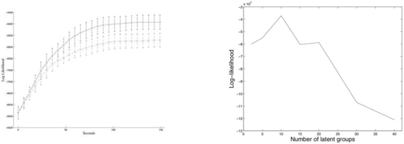
Left: The running time of the naïve variational inference (dashed, red line) against the running time of our enhanced (nested) variational inference algorithm (solid, black line), on a graph with 100 nodes and 4 clusters. Right: The held-out log-likelihood is indicative of the true number of latent clusters, on simulated data. In the example shown, the peak identifies the correct number of clusters, K* = 10.

3.2 Parameter estimation

We compute the empirical Bayes estimates of the model hyper-parameters $\left\{\overrightarrow{\alpha },B\right\}$ with a variational expectation-maximization (EM) algorithm. Alternatives to empirical Bayes have been proposed to fix the hyper-parameters and reduce the computation. The results, however, are not always satisfactory and often times cause of concern, since the inference is sensitive to the choice of the hyper-parameters (Airoldi et al., 2006a). Empirical Bayes, on the other hand, guides the posterior inference towards a region of the hyper-parameter space that is supported by the data.

Variational EM uses the lower bound in Equation 3 as a surrogate for the likelihood. To find a local optimum of the bound, we iterate between: fitting the variational distribution q to approximate the posterior, and maximizing the corresponding lower bound for the likelihood with respect to the parameters. The latter M-step is equivalent to finding the MLE using expected sufficient statistics under the variational distribution. We consider the maximization step for each parameter in turn.

A closed form solution for the approximate maximum likelihood estimate of $\overrightarrow{\alpha }$ does not exist (Minka, 2003). We use a linear-time Newton-Raphson method, where the gradient and Hessian are

$$\begin{array}{l}\frac{\partial {ℒ}_{\overrightarrow{\alpha }}}{\partial {\alpha }_k}=N\left(\psi (\sum _k{\alpha }_k)-\psi ({\alpha }_k)\right)+\sum _p\left(\psi ({\gamma }_{p,k})-\psi (\sum _k{\gamma }_{p,k})\right),\\ \frac{\partial {ℒ}_{\overrightarrow{\alpha }}}{\partial {\alpha }_{k_1}{\alpha }_{k_2}}=N\left({\mathbb{I}}_{(k_1=k_2)}\cdot {\psi }^{\prime }({\alpha }_{k_1})-{\psi }^{\prime }(\sum _k{\alpha }_k)\right).\end{array}$$

The approximate MLE of B is

$$\widehat{B}\left(g,h\right)=\frac{{\sum }_{p,q}R\left(p,q\right)\cdot {\phi }_{p\to qg}{\phi }_{p\leftarrow qh}}{{\sum }_{p,q}{\phi }_{p\to qg}{\phi }_{p\leftarrow qh}},$$ (8)

for every index pair (g, h) ∈ [1, K] × [1, K]. Finally, the approximate MLE of the sparsity parameter ρ is

$$\widehat{\rho }=\frac{{\sum }_{p,q}(1-R(p,q))\cdot ({\sum }_{g,h}{\phi }_{p\to qg}{\phi }_{p\leftarrow qh})}{{\sum }_{p,q}{\sum }_{g,h}{\phi }_{p\to qg}{\phi }_{p\leftarrow qh}}.$$ (9)

Alternatively, we can fix ρ prior to the analysis; the density of the interaction matrix is estimated with d̂ = Σ_p,q R(p, q)/N², and the sparsity parameter is set to ρ̃ = (1 − d̂). This latter estimator attributes all the information in the non-interactions to the point mass, i.e., to latent sources other than the block model B or the mixed membership vectors ${\overrightarrow{\pi }}_{1:N}$. It does however provide a quick recipe to reduce the computational burden during exploratory analyses.³

Several model selection strategies are available for complex hierarchical models. In our setting, model selection translates into the determination of a plausible value of the number of groups K. In the various analyses presented, we selected the optimal value of K with the highest averaged held-out likelihood in a cross-validation experiment, on large networks, and using an approximation to BIC, on small networks.

4 Experiments and Results

Here, we present experiments on simulated data, and we develop two applications to social and protein interaction networks. The three problem settings serve different purposes.

Simulations are performed in Section 4.1 to show that both mixed membership, ${\overrightarrow{\pi }}_{1:N}$, and the latent block structure, B, can be recovered from data, when they exist, and that the nested variational inference algorithm is as fast as the naïve implementation while reaching a higher peak in the likelihood—coeteris paribus.

The application to a friendship network among students in Section 4.2 tests the model on a real data set where we expect a well-defined latent block structure to inform the observed connectivity patterns in the network. In this application, the blocks are interpretable in terms of grades. We compare our results with those that were recently published with a simple mixture of blocks (Doreian et al., 2007) and with a latent space model (Handcock et al., 2007) on the same data.

The application to a protein interaction network in Section 4.3 tests the model on a real data set where we expect a noisy, vague latent block structure to inform the observed connectivity patterns in the network to some degree. In this application, the blocks are interpretable in terms functional biological contexts. This application tests to what extent our model can reduce the dimensionality of the data, while revealing substantive information about the functionality of proteins that can be used to inform subsequent analyses.

4.1 Exploring Expected Model Behavior with Simulations

In developing the MMSB and the corresponding computation, our hope is the the model can recover both the mixed membership of nodes to clusters and the latent block structure among clusters in situations where a block structure exists and the relations are measured with some error. To substantiate this claim, we sampled graphs of 100, 300, and 600 nodes from blockmodels with 4, 10, and 20 clusters, respectively, using the MMSB. We used different values of α to simulate a range of settings in terms of membership of nodes to clusters—from almost unique (α = 0.05) to mixed (α = 0.25).

4.1.1 Recovering the Truth

The variational EM algorithm successfully recovers both the latent block model B and the latent mixed membership vectors ${\overrightarrow{\pi }}_{1:N}$. In Figure 6 we show the adjacency matrices of binary interactions where rows, i.e., nodes, are reordered according to their most likely membership. The nine panels are organized in to a three-by-three grid; panels in the same row correspond to the same combinations of (# nodes and # groups), whereas panels in the same columns correspond to the same value of α that was used to generate the data. In each panel, the estimated reordering of the nodes (i.e., the reordering of rows and columns in the interaction matrix) reveals the block model that was originally used to simulate the interactions. As α increases, each node is likely to belong to more clusters. As a consequence, they express interaction patterns of clusters. This phenomenon reflects in the reordered interaction matrices as the block structure is less evident.

Figure 6.

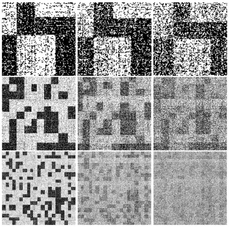
Adjacency matrices of corresponding to simulated interaction graphs with 100 nodes and 4 clusters, 300 nodes and 10 clusters, 600 nodes and 20 clusters (top to bottom) and α equal to 0.05, 0.1 and 0.25 (left to right). Rows, which corresponds to nodes, are reordered according to their most likely membership. The estimated reordering reveals the original blockmodel in all the data settings we tested.

4.1.2 Nested Variational Inference

The nested variational algorithm drives the log-likelihood to converge as fast as the naïve variational inference algorithm does, but reaches a significantly higher plateau. In the left panel of Figure 7, we compare the running times of the nested variational-EM algorithm versus the naïve implementation on a graph with 100 nodes and 4 clusters. We measure the number of seconds on the X axis and the log-likelihood on the Y axis. The two curves are averages over 26 experiments, and the error bars are at three standard deviations. Each of the 26 pairs of experiments was initialized with the same values for the parameters. The nested algorithm, which is more efficient in terms of space, converged faster. Furthermore, the nested variational algorithm can be parallelized given that the updates for each interaction (i, j) are independent of one another.

4.1.3 Choosing the Number of Groups

Figure 7 (right panel) shows an example where cross-validation is sufficient to perform model selection for the MMSB. The example shown corresponds to a network among 300 nodes with K = 10 clusters. We measure the number of latent clusters on the X axis and the average held-out log-likelihood, corresponding to five-fold cross-validation experiments, on the Y axis. A peak in this curve identifies the optimal number of clusters, to the extend of describing the data. The nested variational EM algorithm was run till convergence, for each value of K we tested, with a tolerance of ε = 10⁻⁵. In the example shown, our estimate for K occurs at the peak in the average held-out log-likelihood, and equals the correct number of clusters, K* = 10

4.2 Application to Social Network Analysis

The National Longitudinal Study of Adolescent Health is nationally representative study that explores the how social contexts such as families, friends, peers, schools, neighborhoods, and communities influence health and risk behaviors of adolescents, and their outcomes in young adulthood (Harris et al., 2003; Udry, 2003). Here, we analyze a friendship network among the students, at the same school that was considered by Handcock et al. (2007) and discussants.

A questionnaire was administered to a sample of students who were allowed to nominate up to 10 friends. At the school we picked, friendship nominations were collected among 71 students in grades 7 to 12. Two students did not nominate any friends so we analyzed the network of binary, asymmetric friendship relations among the remaining 69 students. The left panel of Figure 8 shows the raw friendship relations, and we contrast this to the estimated networks in the central and right panels based on our model estimates.

Figure 8.

Original matrix of friensdhip relations among 69 students in grades 7 to 12 (left), and friendship estimated relations obtained by thresholding the posterior expectations ${\overrightarrow{\pi }}_p\prime B{\overrightarrow{\pi }}_q|R$ (center), and ${\overrightarrow{\phi }}_p\prime B{\overrightarrow{\phi }}_q|R$ (right).

Given the size of the network we used BIC to perform model selection, as in the monks example of Section 2.2. The results suggest a model with K* = 6 groups. (We fix K* = 6 in the analyses that follow.) The hyper-parameters were estimated with the nested variational EM. They are α̂ = 0.0487, ρ̂ = 0.936, and a fairly diagonal block-to-block connectivity matrix,

$$\widehat{B}=\left[\begin{array}{llllll}0.3235\hfill & 0.0\hfill & 0.0\hfill & 0.0\hfill & 0.0\hfill & 0.0\hfill \\ 0.0\hfill & 0.3614\hfill & 0.0002\hfill & 0.0\hfill & 0.0\hfill & 0.0\hfill \\ 0.0\hfill & 0.0\hfill & 0.2607\hfill & 0.0\hfill & 0.0\hfill & 0.0002\hfill \\ 0.0\hfill & 0.0\hfill & 0.0\hfill & 0.3751\hfill & 0.0009\hfill & 0.0\hfill \\ 0.0\hfill & 0.0\hfill & 0.0\hfill & 0.0002\hfill & 0.3795\hfill & 0.0\hfill \\ 0.0\hfill & 0.0\hfill & 0.0\hfill & 0.0\hfill & 0.0\hfill & 0.3719\hfill \end{array}\right].$$

Figure 9 shows the expected posterior mixed membership scores for the 69 students in the sample; few students display mixed membership. The rarity of mixed membership in this context is expected. Mixed membership, instead, may signal unexpected social situations for further investigation. For instance, it may signal a family bond such as brotherhood, or a kid that is repeating a grade and is thus part of a broader social clique. In this data set we can successfully attempt an interpretation of the clusters in terms of grades. Table 1 shows the correspondence between clusters and grades in terms of students, for three alternative models. The three models are our mixed membership stochastic blockmodel (MMSB), a simpler stochastic block mixture model (Doreian et al., 2007) (MSB), and the latent space cluster model (Handcock et al., 2007) (LSCM).

Figure 9.

The posterior mixed membership scores, $\overrightarrow{\pi }$, for the 69 students. Each panel correspond to a student; we order the clusters 1 to 6 on the X axis, and we measure the student's grade of membership to these clusters on the Y axis.

Table 1.

Grade levels versus (highest) expected posterior membership for the 69 students, according to three alternative models. MMSB is the proposed mixed membership stochastic blockmodel, MSB is a simpler stochastic block mixture model (Doreian et al., 2007), and LSCM is the latent space cluster model (Handcock et al., 2007).

	MMSB Clusters						MSB Clusters						LSCM Clusters
Grade	1	2	3	4	5	6	1	2	3	4	5	6	1	2	3	4	5	6
7	13	1	0	0	0	0	13	1	0	0	0	0	13	1	0	0	0	0
8	0	9	2	0	0	1	0	10	2	0	0	0	0	11	1	0	0	0
9	0	0	16	0	0	0	0	0	10	0	0	6	0	0	7	6	3	0
10	0	0	0	10	0	0	0	0	0	10	0	0	0	0	0	0	3	7
11	0	0	1	0	11	1	0	0	1	0	11	1	0	0	0	0	3	10
12	0	0	0	0	0	4	0	0	0	0	0	4	0	0	0	0	0	4

Concluding this example, we note how the model decouples the observed friendship patterns into two complementary sources of variability. On the one hand, the connectivity matrix B is a global, unconstrained set of hyper-parameters. On the other hand, the mixed membership vectors ${\overrightarrow{\pi }}_{1:N}$ provide a collection of node-specific latent vectors, which inform the directed connections in the graph in a symmetric fashion—and can be used to produce node-specific predictions.

4.3 Application to Protein Interactions in Saccharomyces Cerevisiae

Protein-protein interactions (PPI) form the physical basis for the formation of complexes and pathways that carry out different biological processes. A number of high-throughput experimental approaches have been applied to determine the set of interacting proteins on a proteome-wide scale in yeast. These include the two-hybrid (Y2H) screens and mass spectrometry methods. Mass spectrometry can be used to identify components of protein complexes (Gavin et al., 2002; Ho et al., 2002).

High-throughput methods, though, may miss complexes that are not present under the given conditions. For example, tagging may disturb complex formation and weakly associated components may dissociate and escape detection. Statistical models that encode information about functional processes with high precision are an essential tool for carrying out probabilistic de-noising of biological signals from high-throughput experiments.

Our goal is to identify the proteins' diverse functional roles by analyzing their local and global patterns of interaction via MMSB. The biochemical composition of individual proteins make them suitable for carrying out a specific set of cellular operations, or functions. Proteins typically carry out these functions as part of stable protein complexes (Krogan et al., 2006). There are many situations in which proteins are believed to interact (Alberts et al., 2002). The main intuition behind our methodology is that pairs of protein interact because they are part of the same stable protein complex, i.e., co-location, or because they are part of interacting protein complexes as they carry out compatible cellular operations.

4.3.1 Gold Standards for Functional Annotations

The Munich Institute for Protein Sequencing (MIPS) database was created in 1998 based on evidence derived from a variety of experimental techniques, but does not include information from high-throughput data sets (Mewes et al., 2004). It contains about 8000 protein complex associations in yeast. We analyze a subset of this collection containing 871 proteins, the interactions amongst which were hand-curated. The institute also provides a set of functional annotations, alternative to the gene ontology (GO). These annotations are organized in a tree, with 15 general functions at the first level, 72 more specific functions at an intermediate level, and 255 annotations at the the leaf level. In Table 2 we map the 871 proteins in our collections to the main functions of the MIPS annotation tree; proteins in our sub-collection have about 2.4 functional annotations on average.⁴

Table 2.

The 15 high-level functional categories obtained by cutting the MIPS annotation tree at the first level and how many proteins (among the 871 we consider) participate in each of them. Most proteins participate in more than one functional category, with an average of ≈ 2.4 functional annotations for each protein.

#	Category	Count
1	Metabolism	125
2	Energy	56
3	Cell cycle & DNA processing	162
4	Transcription (tRNA)	258
5	Protein synthesis	220
6	Protein fate	170
7	Cellular transportation	122
8	Cell rescue, defence & virulence	6
9	Interaction w/ cell. environment	18
10	Cellular regulation	37
11	Cellular other	78
12	Control of cell organization	36
13	Sub-cellular activities	789
14	Protein regulators	1
15	Transport facilitation	41

By mapping proteins to the 15 general functions, we obtain a 15-dimensional representation for each protein. In Figure 10 each panel corresponds to a protein; the 15 functional categories are ordered as in Table 2 on the X axis, whereas the presence or absence of the corresponding functional annotation is displayed on the Y axis.

Figure 10.

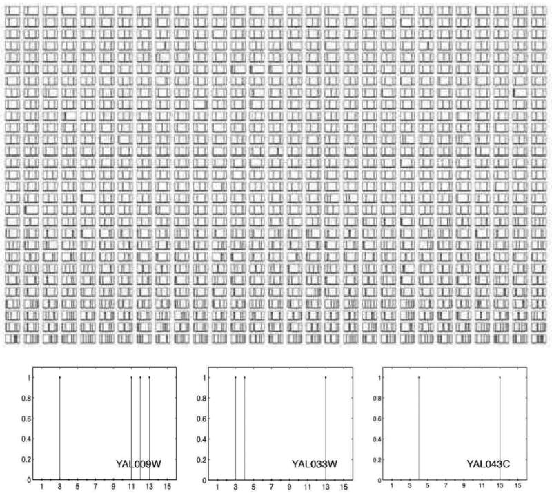
By mapping individual proteins to the 15 general functions in Table 2, we obtain a 15-dimensional representation for each protein. Here, each panel corresponds to a protein; the 15 functional categories are displayed on the X axis, whereas the presence or absence of the corresponding functional annotation is displayed on the Y axis. The plots at the bottom zoom into three example panels (proteins).

4.3.2 Brief Summary of Previous Findings

In previous work, we established the usefulness of an admixture of latent blockmodels for analyzing protein-protein interaction data (Airoldi et al., 2005). For example, we used the MMSB for testing functional interaction hypotheses (by setting a null hypothesis for B), and unsupervised estimation experiments. In the next Section, we assess whether, and how much, functionally relevant biological signal can be captured in by the MMSB.

In summary, the results in Airoldi et al. (2005) show that the MMSB identifies protein complexes whose member proteins are tightly interacting with one another. The identifiable protein complexes correlate with the following four categories of Table 2: cell cycle & DNA processing, transcription, protein synthesis, and sub-cellular activities. The high correlation of inferred protein complexes can be leveraged for predicting the presence of absence of functional annotations, for example, by using a logistic regression. However, there is not enough signal in the data to independently predict annotations in other functional categories. The empirical Bayes estimates of the hyper-parameters that support these conclusions in the various types of analyses are consistent; α̂ < 1 and small; and B̂ nearly block diagonal with two positive blocks comprising the four identifiable protein complexes. In these previous analyses, we fixed the number of latent protein complexes to 15; the number of broad functional categories in Table 2.

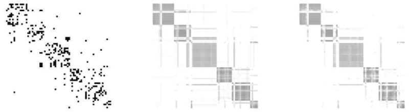
The latent protein complexes are not a-priori identifiable in our model. To resolve this, we estimated a mapping between latent complexes and functions by minimizing the divergence between true and predicted marginal frequencies of membership, where the truth was evaluated on a small fraction of the interactions. We used this mapping to compare predicted versus known functional annotations for all proteins. The best estimated mapping is shown in the left panel of Figure 11, along with the marginal latent category membership, and it is compared to the 15 broad functional categories Table 2, along with the known category membership (in the MIPS database), in the right panel. Figure 12 displays a few examples of predicted mixed membership probabilities against the true annotations, given the estimated mapping of latent protein complexes to functional categories.

Figure 11.

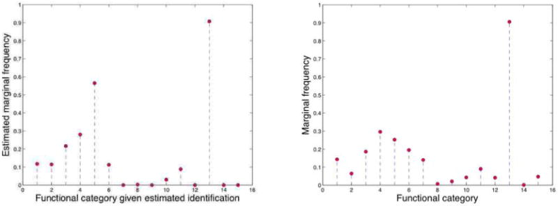
We estimate the mapping of latent groups to functions. The two plots show the marginal frequencies of membership of proteins to true functions (bottom) and to identified functions (top), in the cross-validation experiment. The mapping is selected to maximize the accuracy of the predictions on the training set, in the cross-validation experiment, and to minimize the divergence between marginal true and predicted frequencies if no training data is available—see Section 4.3.2.

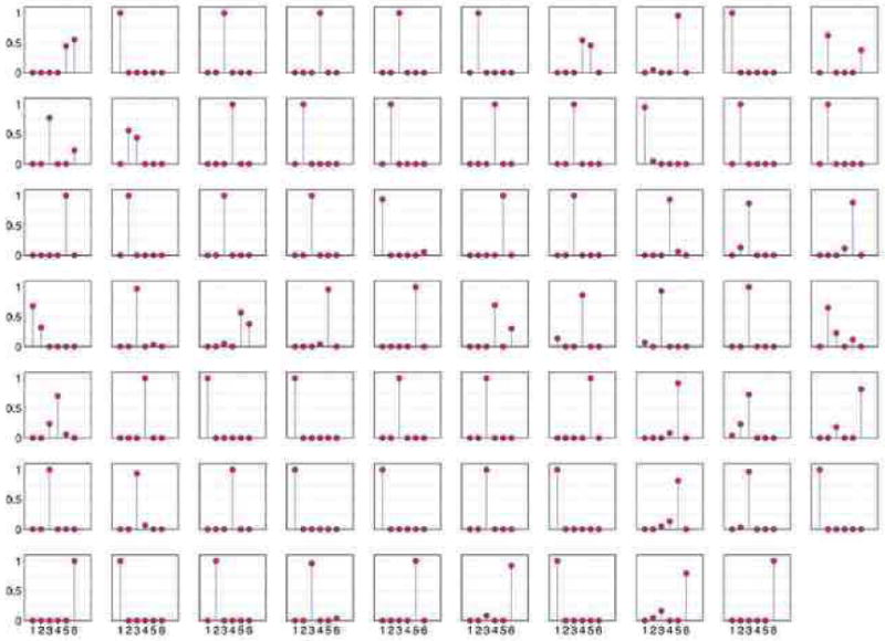
Figure 12.

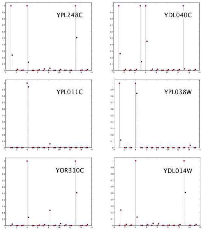
Predicted mixed-membership probabilities (dashed, red lines) versus binary manually curated functional annotations (solid, black lines) for 6 example proteins. The identification of latent groups to functions is estimated, Figure 11.

4.3.3 Measuring the Functional Content in the Posterior

In a follow-up study we considered the gene ontology (GO) (Ashburner et al., 2000) as the source of functional annotations to consider as ground truth in our analyses. GO is a broader and finer grained functional annotation scheme if compared to that produced by the Munich Institute for Protein Sequencing. Furthermore, we explored a much larger model space than in the previous study, in order to tests to what extent MMSB can reduce the dimensionality of the data while revealing substantive information about the functionality of proteins that can be used to inform subsequent analyses. We fit models with a number blocks up to K = 225. Thanks to our nested variational inference algorithm, we were able to perform five-fold cross-validation for each value of K. We determined that a fairly parsimonious model (K* = 50) provides a good description of the observed protein interaction network. This fact is (qualitatively) consistent with the quality of the predictions that were obtained with a parsimonious model (K = 15) in the previous section, in a different setting. This finding supports the hypothesis that groups of interacting proteins in the MIPS data set encode biological signal at a scale of aggregation that is higher than that of protein complexes.⁵

We settled on a model with K* = 50 blocks. To evaluate the functional content of the interactions predicted by such model, we first computed the posterior probabilities of interactions by thresholding the posterior expectations

$$\mathbb{E}\left[R\left(p,q\right)=1\right]\approx {\widehat{\overrightarrow{\pi }}}_p\prime \widehat{B}{\widehat{\overrightarrow{\pi }}}_q\text{and}\mathbb{E}\left[R\left(p,q\right)=1\right]\approx {\widehat{\overrightarrow{\phi }}}_{p\to q}\prime \widehat{B}{\widehat{\overrightarrow{\phi }}}_{p\leftarrow q},$$

and we then computed the precision-recall curves corresponding to these predictions (Myers et al., 2006). These curves are shown in Figure 13 as the light blue (−×) line and the the dark blue (−+) line. In Figure 13 we also plotted the functional content of the original MIPS collection. This plot confirms that the MIPS collection of interactions, our data, is one of the most precise (the Y axis measures precision) and most extensive (the X axis measures the amount of functional annotations predicted, a measure of recall) source of biologically relevant interactions available to date—the yellow diamond, point # 2. The posterior means of $\left({\overrightarrow{\pi }}_{1:N}\right)$ and the estimates of (α, B) provide a parsimonious representation for the MIPS collection, and lead to precise interaction estimates, in moderate amount (the light blue, –× line). The posterior means of (Z_→, Z_←) provide a richer representation for the data, and describe most of the functional content of the MIPS collection with high precision (the dark blue, −+ line). Most importantly, notice the estimated protein interaction networks, i.e., pluses and crosses, corresponding to lower levels of recall feature a more precise functional content than the original. This means that the proposed latent block structure is helpful in summarizing the collection of interactions—by ranking them properly. (It also happens that dense blocks of predicted interactions contain known functional predictions that were not in the MIPS collection.) Table 3 provides more information about three instances of predicted interaction networks displayed in Figure 13; namely, those corresponding the points annotated with the numbers 1 (a collection of interactions predicted with the $\overrightarrow{\pi }$'s), 2 (the original MIPS collection of interactions), and 3 (a collection of interactions predicted with the $\overrightarrow{\phi }$'s). Specifically, the table shows a breakdown of the predicted (posterior) collections of interactions in each example network into the gene ontology categories. A count in the second-to-last column of Table 3 corresponds to the fact that both proteins are annotated with the same GO functional category.⁶ Figure 14 investigates the correlations between the data sets (in rows) we considered in Figure 13 and few gene ontology categories (in columns). The intensity of the square (red is high) measures the area under the precision-recall curve (Myers et al., 2006).

Figure 13.

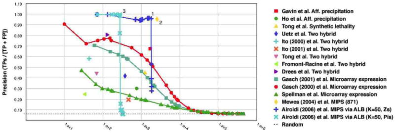
In the top panel we measure the functional content of the the MIPS collection of protein interactions (yellow diamond), and compare it against other published collections of interactions and microarray data, and to the posterior estimates of the MMSB models—computed as described in Section 4.3.3. A breakdown of three estimated interaction networks (the points annotated 1, 2, and 3) into most represented gene ontology categories is detailed in Table 3.

Table 3.

Breakdown of three example interaction networks into most represented gene ontology categories—see text for more details. The digit in the first column indicates the example network in Figure 13 that any given line refers to. The last two columns quote the number of predicted, and possible pairs for each GO term.

#	GO Term	Description	Pred.	Tot.
1	GO:0043285	Biopolymer catabolism	561	17020
1	GO:0006366	Transcription from RNA polymerase II promoter	341	36046
1	GO:0006412	Protein biosynthesis	281	299925
1	GO:0006260	DNA replication	196	5253
1	GO:0006461	Protein complex assembly	191	11175
1	GO:0016568	Chromatin modification	172	15400
1	GO:0006473	Protein amino acid acetylation	91	666
1	GO:0006360	Transcription from RNA polymerase I promoter	78	378
1	GO:0042592	Homeostasis	78	5778
2	GO:0043285	Biopolymer catabolism	631	17020
2	GO:0006366	Transcription from RNA polymerase II promoter	414	36046
2	GO:0016568	Chromatin modification	229	15400
2	GO:0006260	DNA replication	226	5253
2	GO:0006412	Protein biosynthesis	225	299925
2	GO:0045045	Secretory pathway	151	18915
2	GO:0006793	Phosphorus metabolism	134	17391
2	GO:0048193	Golgi vesicle transport	128	9180
2	GO:0006352	Transcription initiation	121	1540
3	GO:0006412	Protein biosynthesis	277	299925
3	GO:0006461	Protein complex assembly	190	11175
3	GO:0009889	Regulation of biosynthesis	28	990
3	GO:0051246	Regulation of protein metabolism	28	903
3	GO:0007046	Ribosome biogenesis	10	21528
3	GO:0006512	Ubiquitin cycle	3	2211

Figure 14.

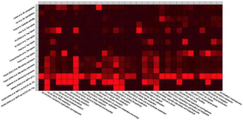
We investigate the correlations between data collections (rows) and a sample of gene ontology categories (columns). The intensity of the square (red is high) measures the area under the precision-recall curve.

In this application, the MMSB learned information about (i) the mixed membership of objects to latent groups, and (ii) the connectivity patterns among latent groups. These quantities were useful in describing and summarizing the functional content of the MIPS collection of protein interactions. This suggests the use of MMSB as a dimensionality reduction approach that may be useful for performing model-driven denoising of new collections of interactions, such as those measured via high-throughput experiments.

5 Discussion

Below we place our research in a larger modeling context, offer some insights into the inner workings of the model, and briefly comment on limitations and extensions.

Modern probabilistic models for relational data analysis are rooted in the stochastic blockmodels for psychometric and sociological analysis, pioneered by Lorrain and White (1971) and by Holland and Leinhardt (1975). In statistics, this line of research has been extended in various contexts over the years (Fienberg et al., 1985; Wasserman and Pattison, 1996; Snijders, 2002; Hoff et al., 2002; Doreian et al., 2004). In machine learning, the related technique of Markov random networks (Frank and Strauss, 1986) have been used for link prediction (Taskar et al., 2003) and the traditional blockmodels have been extended to include nonparametric Bayesian priors (Kemp et al., 2004, 2006) and to integrate relations and text (McCallum et al., 2007).

There is a particularly close relationship between the MMSB and the latent space models (Hoff et al., 2002; Handcock et al., 2007). In the latent space models, the latent vectors are drawn from Gaussian distributions and the interaction data is drawn from a Gaussian with mean ${\overrightarrow{\pi }}_p\prime \mathbb{I}{\overrightarrow{\pi }}_q$. In the MMSB, the marginal probability of an interaction takes a similar form, ${\overrightarrow{\pi }}_p\prime B{\overrightarrow{\pi }}_q$, where B is the matrix of probabilities of interactions for each pair of latent groups. Two major differences exist between these approaches. In MMSB, the distribution over the latent vectors is a Dirichlet and the underlying data distribution is arbitrary—we have chosen Bernoulli. The posterior inference in latent space models (Hoff et al., 2002; Handcock et al., 2007) is carried out via MCMC sampling, while we have developed a scalable variational inference algorithm to analyze large network structures. (It would be interesting to develop a variational algorithm for the latent space models as well.)

We note how the model decouples the observed friendship patterns into two complementary sources of variability. On the one hand, the connectivity matrix B is a global, unconstrained set of hyper-parameters. On the other hand, the mixed membership vectors ${\overrightarrow{\pi }}_{1:N}$ provide a collection of node-specific latent vectors, which inform the directed connections in the graph in a symmetric fashion. Last, the single membership indicators $({\overrightarrow{z}}_{p\to q},{\overrightarrow{z}}_{p\leftarrow q})$ provide a collection interaction-specific latent variables.

A recurring question, which bears relevance to mixed membership models in general, is why we do not integrate out the single membership indicators— $({\overrightarrow{z}}_{p\to q},{\overrightarrow{z}}_{p\leftarrow q})$. While this may lead to computational efficiencies we would often lose interpretable quantities that are useful for making predictions, for de-noising new measurements, or for performing other tasks. In fact, the posterior distributions of such quantities typically carry substantive information about elements of the application at hand. In the application to protein interaction networks of Section 4.3, for example, they encode the interaction-specific memberships of individual proteins to protein complexes.

A limitation of our model can be best appreciated in a simulation setting. If we consider structural properties of the network MMSB is capable of generating, we count a wide array of local and global connectivity patterns. But the model does not readily generate hubs, that is, nodes connected with a large number of directed or undirected connections, or networks with skewed degree distributions.

From a data analysis perspective, we speculate that the value of MMSB in capturing substantive information about a problem will increase in semi-supervised setting—where, for example, information about the membership of genes to functional contexts is included in the form of prior distributions. In such a setting we may be interested in looking at the change between prior and posterior membership; a sharp change may signal biological phenomena worth investigating.

We need not assume that the number of groups/blocks, K, is finite. It is possible, for example, to posit that the mixed-membership vectors are sampled form a stochastic process D_α, in the nonparametric setting. In particular, in order to maintain mixed membership of nodes to groups/blocks we need to sample them from a hierarchical Dirichlet process (Teh et al., 2006), rather than from a Diriclet Process (Escobar and West, 1995).

6 Conclusions

In this paper we introduced mixed membership stochastic blockmodels, a novel class of latent variable models for relational data. These models provide exploratory tools for scientific analyses in applications where the observations can be represented as a collection of unipartite graphs. The nested variational inference algorithm is parallelizable and allows fast approximate inference on large graphs.

The relational nature of such data as well as the multiple goals of the analysis in the applications we considered motivated our technical choices. Latent variables in our models are introduced to capture application-specific substantive elements of interest, e.g., monks and factions in the monastery. The applications to social and biological networks we considered share considerable similarities in the way such elements relate. This allowed us to identify a general formulation of the model that we present in Appendix A. Approximate variational inference for the general model is presented in Appendix B.

A General Model Formulation

In general, mixed membership stochastic blockmodels can be specified in terms of assumptions at four levels: population, node, latent variable, and sampling scheme level.

A1–Population Level

Assume that there are K classes or sub-populations in the population of interest. We denote by f ( R(p, q) | B(g, h) ) the probability distribution of the relation measured on the pair of nodes (p, q), where the p-th node is in the h-th sub-population, the q-th node is in the h-th sub-population, and B(g, h) contains the relevant parameters. The indices i, j run in 1, …, N, and the indices g, h run in 1, …, K.

A2—Node Level

The components of the membership vector ${\overrightarrow{\pi }}_p={[{\overrightarrow{\pi }}_p(1),\dots ,{\overrightarrow{\pi }}_p(k)]}^{\prime }$ encodes the mixed membership of the n-th node to the various sub-populations. The distribution of the observed response R(p, q) given the relevant, node-specific memberships, $({\overrightarrow{\pi }}_p,{\overrightarrow{\pi }}_q)$, is then

$$\mathit{\text{Pr}}(R\left(p,q\right)|{\overrightarrow{\pi }}_p,{\overrightarrow{\pi }}_q,B)=\sum _{g,h=1}^K{\overrightarrow{\pi }}_p\left(g\right)f\left(R\left(p,q\right)|B\left(g,h\right)\right){\overrightarrow{\pi }}_q\left(h\right).$$ (10)

Conditional on the mixed memberships, the response edges y_jnm are independent of one another, both across distinct graphs and pairs of nodes.

A3—Latent Variable Level

Assume that the mixed membership vectors ${\overrightarrow{\pi }}_{1:N}$ are realizations of a latent variable with distribution $D_{\overrightarrow{\alpha }}$, with parameter vector $\overrightarrow{\alpha }$. The probability of observing R(p, q), given the parameters, is then

$$\mathit{\text{Pr}}\left(R\left(p,q\right)|\overrightarrow{\alpha },B\right)=\mathit{\int }\mathit{\text{Pr}}(R\left(p,q\right)|{\overrightarrow{\pi }}_p,{\overrightarrow{\pi }}_q,B)D_{\overrightarrow{\alpha }}\left(d\overrightarrow{\pi }\right).$$ (11)

A4—Sampling Scheme Level

Assume that the M independent replications of the relations measured on the population of nodes are independent of one another. The probability of observing the whole collection of graphs, R_1:M, given the parameters, is then given by the following equation.

$$\mathit{\text{Pr}}(R_{1:M}|\overrightarrow{\alpha },B)=\prod _{m=1}^M\prod _{p,q=1}^N\mathit{\text{Pr}}(R_m\left(p,q\right)|\overrightarrow{\alpha },B).$$ (12)

Full model specifications immediately adapt to the different kinds of data, e.g., multiple data types through the choice of f, or parametric or semi-parametric specifications of the prior on the number of clusters through the choice of D_α.

B Details of the Variational Approximation

Here we present more details about the derivation of the variational EM algorithm presented in Section 3. Furthermore, we address a setting where M replicates are available about the paired measurements, G_1:M = (N, R_1:M), and relations R_m(p, q) take values into an arbitrary metric space according to f ( R_m(p, q) | .. ). An extension of the inference algorithm to address the case or multivariate relations, say J-dimensional, and multiple blockmodels B_1:J each corresponding to a distinct relational response, can be derived with minor modifications of the derivations that follow.

B.1 Variational Expectation-Maximization

We begin by briefly summarizing the general strategy we intend to use. The approximate variant of EM we describe here is often referred to as Variational EM (Beal and Ghahramani, 2003). We begin by rewriting Y = R for the data, $X=\left({\overrightarrow{\pi }}_{1:N},Z_{\to },Z_{\leftarrow }\right)$ for the latent variables, and $\mathrm{\Theta }=\left(\overrightarrow{\alpha },B\right)$ for the model's parameters. Briefly, it is possible to lower bound the likelihood, p(Y|Θ), making use of Jensen's inequality and of any distribution on the latent variables q(X),

$$\begin{array}{l}p\left(Y|\mathrm{\Theta }\right)=log{\mathit{\int }}_{\chi }p\left(Y,X|\mathrm{\Theta }\right)dX\\ =log{\mathit{\int }}_{\chi }q\left(X\right)\frac{p\left(Y,X|\mathrm{\Theta }\right)}{q\left(X\right)}dX\left(\text{for any}q\right)\\ \ge {\mathit{\int }}_{\chi }q\left(X\right)log\frac{p\left(Y,X|\mathrm{\Theta }\right)}{q\left(X\right)}dX\left(\text{Jensen's}\right)\\ ={\mathbb{E}}_q\left[logp\left(Y,X|\mathrm{\Theta }\right)-logq\left(X\right)\right]=:ℒ\left(q,\mathrm{\Theta }\right)\end{array}$$ (13)

In EM, the lower bound $ℒ(q,\mathrm{\Theta })$ is then iteratively maximized with respect to Θ, in the M step, and q in the E step (Dempster et al., 1977). In particular, at the t-th iteration of the E step we set

$$q^{\left(t\right)}=p(X|Y,{\mathrm{\Theta }}^{\left(t-1\right)}),$$ (14)

that is, equal to the posterior distribution of the latent variables given the data and the estimates of the parameters at the previous iteration.

Unfortunately, we cannot compute the posterior in Equation 14 for the admixture of latent blocks model. Rather, we define a direct parametric approximation to it, q̃ = q_Δ(X), which involves an extra set of variational parameters, Δ, and entails an approximate lower bound for the likelihood ${ℒ}_{\mathrm{\Delta }}(q,\mathrm{\Theta })$. At the t-th iteration of the E step, we then minimize the Kullback-Leibler divergence between q^(t) and $q_{\mathrm{\Delta }}^{\left(t\right)}$, with respect to Δ, using the data.⁷ The optimal parametric approximation is, in fact, a proper posterior as it depends on the data Y, although indirectly, $q^{\left(t\right)}\approx q_{\mathrm{\Delta }\ast \left(Y\right)}^{\left(t\right)}\left(X\right)=p\left(X|Y\right)$.

B.2 Lower Bound for the Likelihood

According to the mean-field theory (Jordan et al., 1999; Xing et al., 2003), one can approximate an intractable distribution such as the one defined by Equation (1) by a fully factored distribution $q\left({\overrightarrow{\pi }}_{1:N},Z_{1:M}^{\to },Z_{1:M}^{\leftarrow }\right)$ defined as follows:

$$\begin{array}{l}q({\overrightarrow{\pi }}_{1:N},Z_{1:M}^{\to },Z_{1:M}^{\leftarrow }|{\overrightarrow{\gamma }}_{1:N},{\mathrm{\Phi }}_{1:M}^{\to },{\mathrm{\Phi }}_{1:M}^{\leftarrow })\\ =\prod _p{q}_1({\overrightarrow{\pi }}_p|{\overrightarrow{\gamma }}_p)\prod _m\prod _{p,q}\left(q_2({\overrightarrow{z}}_{p\to q}^m|{\overrightarrow{\phi }}_{p\to q}^m,1)q_2({\overrightarrow{z}}_{p\leftarrow q}^m|{\overrightarrow{\phi }}_{p\leftarrow q}^m,1)\right),\end{array}$$ (15)

where q₁ is a Dirichlet, q₂ is a multinomial, and $\mathrm{\Delta }=({\overrightarrow{\gamma }}_{1:N},{\mathrm{\Phi }}_{1:M}^{\to },{\mathrm{\Phi }}_{1:M}^{\leftarrow })$ represent the set of free variational parameters need to be estimated in the approximate distribution.

Minimizing the Kulback-Leibler divergence between this $q({\overrightarrow{\pi }}_{1:N},Z_{1:M}^{\to },Z_{1:M}^{\leftarrow }|\mathrm{\Delta })$ and the original $p({\overrightarrow{\pi }}_{1:N},Z_{1:M}^{\to },Z_{1:M}^{\leftarrow }$ defined by Equation (1) leads to the following approximate lower bound for the likelihood.

$$\begin{array}{l}{ℒ}_{\mathrm{\Delta }}(q,\mathrm{\Theta })={\mathbb{E}}_q[log\prod _m\prod _{p,q}{p}_1(R_m(p,q)|{\overrightarrow{z}}_{p\to q}^m,{\overrightarrow{z}}_{p\leftarrow q}^m,B)]\\ +{\mathbb{E}}_q[log\prod _m\prod _{p,q}{p}_2({\overrightarrow{z}}_{p\to q}^m|{\overrightarrow{\pi }}_p,1)]+{\mathbb{E}}_q[log\prod _m\prod _{p,q}{p}_2({\overrightarrow{z}}_{p\leftarrow q}^m|{\overrightarrow{\pi }}_q,1)]\\ +{\mathbb{E}}_q[log\prod _p{p}_3({\overrightarrow{\pi }}_p|\overrightarrow{\alpha })]-{\mathbb{E}}_q[\prod _p{q}_1({\overrightarrow{\pi }}_p|{\overrightarrow{\gamma }}_p)]\\ -{\mathbb{E}}_q[log\prod _m\prod _{p,q}{q}_2({\overrightarrow{z}}_{p\to q}^m|{\overrightarrow{\phi }}_{p\to q}^m,1)]-{\mathbb{E}}_q[log\prod _m\prod _{p,q}{q}_2({\overrightarrow{z}}_{p\leftarrow q}^m|{\overrightarrow{\phi }}_{p\leftarrow q}^m,1)].\end{array}$$

Working on the single expectations leads to

$$\begin{array}{l}{ℒ}_{\mathrm{\Delta }}(q,\mathrm{\Theta })=\sum _m\sum _{p,q}\sum _{g,h}{\phi }_{p\to q,g}^m{\phi }_{p\leftarrow q,h}^m\cdot f(R_m(p,q),B(g,h))\\ +\sum _m\sum _{p,q}\sum _g{\phi }_{p\to q,g}^m[\psi ({\gamma }_{p,g})-\psi (\sum _g{\gamma }_{p,g})]\\ +\sum _m\sum _{p,q}\sum _h{\phi }_{p\leftarrow q,h}^m[\psi ({\gamma }_{p,h})-\psi (\sum _h{\gamma }_{p,h})]\\ +\sum _{p}log\mathrm{\Gamma }(\sum _k{\alpha }_k)-\sum _{p,k}log\mathrm{\Gamma }({\alpha }_k)+\sum _{p,k}({\alpha }_k-1)[\psi ({\gamma }_{p,k})-\psi (\sum _k{\gamma }_{p,k})]\\ -\sum _{p}log\mathrm{\Gamma }(\sum _k{\gamma }_{p,k})+\sum _{p,k}log\mathrm{\Gamma }({\gamma }_{p,k})-\sum _{p,k}({\gamma }_{p,k}-1)[\psi ({\gamma }_{p,k})-\psi (\sum _k{\gamma }_{p,k})]\\ -\sum _m\sum _{p,q}\sum _g{\phi }_{p\to q,g}^{m}log{\phi }_{p\to q,g}^m-\sum _m\sum _{p,q}\sum _h{\phi }_{p\leftarrow q,h}^{m}log{\phi }_{p\leftarrow q,h}^m\end{array}$$

where

$$f\left(R_m\left(p,q\right),B\left(g,h\right)\right)=R_m\left(p,q\right)logB\left(g,h\right)+\left(1-R_m\left(p,q\right)\right)log\left(1-B\left(g,h\right)\right);$$

m runs over 1, …, M; p, q run over 1, …, N; g, h, k run over 1, …, K; and ψ(x) is the derivative of the log-gamma function, $\frac{dlog\mathrm{\Gamma }\left(x\right)}{dx}$.

B.3 The Expected Value of the Log of a Dirichlet Random Vector

The computation of the lower bound for the likelihood requires us to evaluate ${\mathbb{E}}_q[log{\overrightarrow{\pi }}_p]$ for p = 1, …, N. Recall that the density of an exponential family distribution with natural parameter $\overrightarrow{\theta }$ can be written as

$$\begin{array}{l}p(x|\alpha )=h(x)\cdot c(\alpha )\cdot exp\{\sum _k{\theta }_k(\alpha )\cdot t_k(x)\}\\ =h(x)\cdot exp\{\sum _k{\theta }_k(\alpha )\cdot t_k(x)-logc(\alpha )\}.\end{array}$$

Omitting the node index p for convenience, we can rewrite the density of the Dirichlet distribution p₃ as an exponential family distribution,

$$p_3\left(\overrightarrow{\pi }|\overrightarrow{\alpha }\right)=exp\left\{\sum _k\left({\alpha }_k-1\right)log\left({\pi }_k\right)-log\frac{{\prod }_k\mathrm{\Gamma }\left({\alpha }_k\right)}{\mathrm{\Gamma }\left({\sum }_k{\alpha }_k\right)}\right\},$$

with natural parameters ${\theta }_k(\overrightarrow{\alpha })=({\alpha }_k-1)$ and natural sufficient statistics $t_k(\overrightarrow{\pi })=log({\pi }_k)$. Let $c^{\prime }(\overrightarrow{\theta })=c({\alpha }_1(\overrightarrow{\theta }),\dots ,{\alpha }_K(\overrightarrow{\theta }))$; using a well known property of the exponential family distributions Schervish (1995) we find that

$${\mathbb{E}}_q\left[log{\pi }_k\right]={\mathbb{E}}_{\overrightarrow{\theta }}\left[log{t}_k(x)\right]=\psi ({\alpha }_k)-\psi (\sum _k{\alpha }_k),$$

where ψ(x) is the derivative of the log-gamma function, $\frac{dlog\mathrm{\Gamma }\left(x\right)}{dx}$.

B.4 Variational E Step

The approximate lower bound for the likelihood ${ℒ}_{\mathrm{\Delta }}(q,\mathrm{\Theta })$ can be maximized using exponential family arguments and coordinate ascent Wainwright and Jordan (2003).

Isolating terms containing ${\phi }_{p\to q,g}^m$ and ${\phi }_{p\leftarrow q,h}^m$ we obtain ${ℒ}_{{\phi }_{p\to q,g}^m}\left(q,\mathrm{\Theta }\right)$ and ${ℒ}_{{\phi }_{p\to q,g}^m}\left(q,\mathrm{\Theta }\right)$. The natural parameters ${\overrightarrow{g}}_{p\to q}^m$ and ${\overrightarrow{g}}_{p\leftarrow q}^m$ corresponding to the natural sufficient statistics $log({\overrightarrow{z}}_{p\to q}^m)$ and $log({\overrightarrow{z}}_{p\leftarrow q}^m)$ are functions of the other latent variables and the observations. We find that

$$\begin{array}{c}{g}_{p\to q,g}^m=log{\pi }_{p,g}+\sum _h{z}_{p\leftarrow q,h}^m\cdot f\left(R_m\left(p,q\right),B\left(g,h\right)\right),\\ g_{p\leftarrow q,h}^m=log{\pi }_{q,h}+\sum _g{z}_{p\to q,g}^m\cdot f\left(R_m\left(p,q\right),B\left(g,h\right)\right),\end{array}$$

for all pairs of nodes (p, q) in the m-th network; where g, h = 1, …, K, and

$$f\left(R_m\left(p,q\right),B\left(g,h\right)\right)=R_m\left(p,q\right)logB\left(g,h\right)+\left(1-R_m\left(p,q\right)\right)log\left(1-B\left(g,h\right)\right).$$

This leads to the following updates for the variational parameters $({\overrightarrow{\phi }}_{p\to q}^m,{\overrightarrow{\phi }}_{p\leftarrow q}^m)$, for a pair of nodes (p, q) in the m-th network:

$$\begin{array}{l}{\widehat{\phi }}_{p\to q,g}^m\propto e^{{\mathbb{E}}_q\left[g_{p\to q,g}^m\right]}\\ =e^{{\mathbb{E}}_q\left[log{\pi }_{p,g}\right]}\cdot e^{{\sum }_h{\phi }_{p\leftarrow q,h}^m\cdot {\mathbb{E}}_q\left[f\left(R_m\left(p,q\right),B\left(g,h\right)\right)\right]}\\ =e^{{\mathbb{E}}_q\left[log{\pi }_{p,g}\right]}\cdot \prod _h{\left(B{\left(g,h\right)}^{R_m\left(p,q\right)}\cdot {\left(1-B\left(g,h\right)\right)}^{1-R_m\left(p,q\right)}\right)}^{{\phi }_{p\leftarrow q,h}^m},\end{array}$$ (16)

$$\begin{array}{l}{\widehat{\phi }}_{p\leftarrow q,h}^m\propto e^{{\mathbb{E}}_q\left[g_{p\leftarrow q,h}^m\right]}\\ =e^{{\mathbb{E}}_q\left[log{\pi }_{q,h}\right]}\cdot e^{{\sum }_g{\phi }_{p\to q,g}^m\cdot {\mathbb{E}}_q\left[f\left(R_m\left(p,q\right),B\left(g,h\right)\right)\right]}\\ =e^{{\mathbb{E}}_q\left[log{\pi }_{q,h}\right]}\cdot \prod _g{\left(B{\left(g,h\right)}^{R_m\left(p,q\right)}\cdot {\left(1-B\left(g,h\right)\right)}^{1-R_m\left(p,q\right)}\right)}^{{\phi }_{p\to q,g}^m},\end{array}$$ (17)

for g, h = 1, …, K. These estimates of the parameters underlying the distribution of the nodes' group indicators ${\overrightarrow{\phi }}_{p\to q}^m$ and ${\overrightarrow{\phi }}_{p\leftarrow q}^m$ need be normalized, to make sure ${\sum }_k{\phi }_{p\to q,k}^m={\sum }_k{\phi }_{p\leftarrow q,k}^m=1$.

Isolating terms containing γ_p,k we obtain ${ℒ}_{{\gamma }_{p,k}}\left(q,\mathrm{\Theta }\right)$. Setting $\frac{\partial {ℒ}_{{\gamma }_{p,k}}}{\partial {\gamma }_{p,k}}$ equal to zero and solving for γ_p,k yields:

$${\widehat{\gamma }}_{p,k}={\alpha }_k+\sum _m\sum _q{\phi }_{p\to q,k}^m+\sum _m\sum _q{\phi }_{p\leftarrow q,k}^m,$$ (18)

for all nodes $p\in \mathcal{P}$ and k = 1, …, K.

The t-th iteration of the variational E step is carried out for fixed values of ${\mathrm{\Theta }}^{\left(t-1\right)}=({\overrightarrow{\alpha }}^{\left(t-1\right)},B^{\left(t-1\right)})$, and finds the optimal approximate lower bound for the likelihood ${ℒ}_{\mathrm{\Delta }\ast }(q,{\mathrm{\Theta }}^{\left(t-1\right)})$.

B.5 Variational M Step

The optimal lower bound ${ℒ}_{\mathrm{\Delta }\ast }(q^{\left(t-1\right)},\mathrm{\Theta })$ provides a tractable surrogate for the likelihood at the t-th iteration of the variational M step. We derive empirical Bayes estimates for the hyper-parameters Θ that are based upon it.⁸ That is, we maximize ${ℒ}_{\mathrm{\Delta }\ast }(q^{\left(t-1\right)},\mathrm{\Theta })$ with respect to Θ, given expected sufficient statistics computed using ${ℒ}_{\mathrm{\Delta }\ast }(q^{\left(t-1\right)},{\mathrm{\Theta }}^{\left(t-1\right)})$.

Isolating terms containing $\overrightarrow{\alpha }$ we obtain ${ℒ}_{\overrightarrow{\alpha }}\left(q,\Theta \right)$. Unfortunately, a closed form solution for the approximate maximum likelihood estimate of $\overrightarrow{\alpha }$ does not exist Blei et al. (2003). We can produce a Newton-Raphson method that is linear in time, where the gradient and Hessian for the bound ${ℒ}_{\overrightarrow{\alpha }}$ are

$$\begin{array}{l}\frac{\partial {ℒ}_{\overrightarrow{\alpha }}}{\partial {\alpha }_k}=N\left(\psi (\sum _k{\alpha }_k)-\psi ({\alpha }_k)\right)+\sum _p\left(\psi ({\gamma }_{p,k})-\psi (\sum _k{\gamma }_{p,k})\right),\\ \frac{\partial {ℒ}_{\overrightarrow{\alpha }}}{\partial {\alpha }_{k_1}{\alpha }_{k_2}}=N\left({\mathbb{I}}_{\left(k_1=k_2\right)}\cdot {\psi }^{\prime }({\alpha }_{k_1})-{\psi }^{\prime }(\sum _k{\alpha }_k)\right).\end{array}$$

Isolating terms containing B we obtain ${ℒ}_B$, whose approximate maximum is

$$\widehat{B}\left(g,h\right)=\frac{1}{M}\sum _m\left(\frac{{\sum }_{p,q}{R}_m\left(p,q\right)\cdot {\phi }_{p\to qg}^m{\phi }_{p\leftarrow gh}^m}{{\sum }_{p,q}{\phi }_{p\to qg}^m{\phi }_{p\leftarrow qh}^m}\right),$$ (19)

for every index pair (g, h) ∈ [1, K] × [1, K].

In Section 2.1 we introduced an extra parameter, ρ, to control the relative importance of presence and absence of interactions in likelihood, i.e., the score that informs inference and estimation. Isolating terms containing ρ we obtain ${ℒ}_{\rho }$. We may then estimate the sparsity parameter ρ by

$$\widehat{\rho }=\frac{1}{M}\sum _m\left(\frac{{\sum }_{p,q}\left(1-R_m\left(p,q\right)\right)\cdot \left({\sum }_{g,h}{\phi }_{p\to qg}^m{\phi }_{p\leftarrow qh}^m\right)}{{\sum }_{p,q}{\sum }_{g,h}{\phi }_{p\to qg}^m{\phi }_{p\leftarrow qh}^m}\right).$$ (20)

Alternatively, we can fix ρ prior to the analysis; the density of the interaction matrix is estimated with d̂ = Σ_m,p,q R_m(p, q)/(N²M), and the sparsity parameter is set to ρ̃ = (1 − d̂). This latter estimator attributes all the information in the non-interactions to the point mass, i.e., to latent sources other than the block model B or the mixed membership vectors ${\overrightarrow{\pi }}_{1:N}$. It does, however, provide a quick recipe to reduce the computational burden during exploratory analyses.⁹

References

- Airoldi EM, Blei DM, Xing EP, Fienberg SE. ACM SIGKDD Workshop on Link Discovery: Issues, Approaches and Applications. 2005. A latent mixed-membership model for relational data. [Google Scholar]
- Airoldi EM, Fienberg SE, Joutard C, Love TM. Technical Report CMU-ML-06-101. School of Computer Science, Carnegie Mellon University; Apr, 2006a. Discovering latent patterns with hierarchical Bayesian mixed-membership models and the issue of model choice. [Google Scholar]
- Airoldi EM, Fienberg SE, Xing EP. Biological context analysis of gene expression data. Jun, 2006b. Manuscript. [Google Scholar]
- Alberts B, Johnson A, Lewis J, Raff M, Roberts K, Walter P. Molecular Biology of the Cell. 4th. Garland: 2002. [Google Scholar]
- Ashburner M, Ball CA, Blake JA, Botstein D, Butler H, Cherry JM, Davis AP, Dolinski K, Dwight SS, Eppig JT, Harris MA, Hill DP, Issel-Tarver L, Kasarskis A, Lewis S, Matese JC, Richardson JE, Ringwald M, Rubinand GM, Sherlock G. Gene ontology: Tool for the unification of biology. The gene ontology consortium. Nature Genetics. 2000;25(1):25–29. doi: 10.1038/75556. [DOI] [PMC free article] [PubMed] [Google Scholar]
- Beal MJ, Ghahramani Z. The variational Bayesian EM algorithm for incomplete data: With application to scoring graphical model structures. In: Bernardo JM, Bayarri MJ, Berger JO, Dawid AP, Heckerman D, Smith AFM, West M, editors. Bayesian Statistics. Vol. 7. Oxford University Press; 2003. pp. 453–464. [Google Scholar]
- Berkman L, Singer BH, Manton K. Black/white differences in health status and mortality among the elderly. Demography. 1989;26(4):661–678. [PubMed] [Google Scholar]
- Bishop C, Spiegelhalter D, Winn J. VIBES: A variational inference engine for Bayesian networks. In: Becker S, Thrun S, Obermayer K, editors. Advances in Neural Information Processing Systems 15. MIT Press; Cambridge, MA: 2003. pp. 777–784. [Google Scholar]
- Blei DM, Ng A, Jordan MI. Latent Dirichlet allocation. Journal of Machine Learning Research. 2003;3:993–1022. [Google Scholar]
- Bradley RT. Charisma and Social Structure. Paragon House; 1987. [Google Scholar]
- Breiger RL, Boorman SA, Arabie P. An algorithm for clustering relational data with applications to social network analysis and comparison to multidimensional scaling. Journal of Mathematical Psychology. 1975;12:328–383. [Google Scholar]
- Buntine WL, Jakulin A. Discrete components analysis. In: Saunders C, Grobelnik M, Gunn S, Shawe-Taylor J, editors. Subspace, Latent Structure and Feature Selection Techniques. Springer-Verlag; 2006. to appear. [Google Scholar]
- Davis GB, Carley KM. Clearing the FOG: Fuzzy, overlapping groups for social networks. 2006. Manuscript. [Google Scholar]
- Dempster A, Laird N, Rubin D. Maximum likelihood from incomplete data via the EM algorithm. Journal of the Royal Statistical Society, Series B. 1977;39:1–38. [Google Scholar]
- Doreian P, Batagelj V, Ferligoj A. Generalized Blockmodeling. Cambridge University Press; 2004. [Google Scholar]
- Doreian P, Batagelj V, Ferligoj A. Discussion of “Model-based clustering for social networks”. Journal of the Royal Statistical Society, Series A. 2007;170 [Google Scholar]
- Erosheva EA. PhD thesis. Carnegie Mellon University, Department of Statistics; 2002. Grade of membership and latent structure models with application to disability survey data. [Google Scholar]
- Erosheva EA, Fienberg SE. Bayesian mixed membership models for soft clustering and classification. In: Weihs C, Gaul W, editors. Classification—The Ubiquitous Challenge. Springer-Verlag; 2005. pp. 11–26. [Google Scholar]
- Escobar M, West M. Bayesian density estimation and inference using mixtures. Journal of the American Statistical Association. 1995;90:577–588. [Google Scholar]
- Fienberg SE, Meyer MM, Wasserman S. Statistical analysis of multiple sociometric relations. Journal of the American Statistical Association. 1985;80:51–67. [Google Scholar]
- Frank O, Strauss D. Markov graphs. Journal of the American Statistical Association. 1986;81:832–842. [Google Scholar]
- Gavin AC, Bosche M, Krause R, Grandi P, Marzioch M, Bauer A, Schultz J, et al. Functional organization of the yeast proteome by systematic analysis of protein complexes. Nature. 2002;415:141–147. doi: 10.1038/415141a. [DOI] [PubMed] [Google Scholar]
- Griffiths TL, Steyvers M. Finding scientific topics. Proceedings of the National Academy of Sciences. 2004;101 1:5228–5235. doi: 10.1073/pnas.0307752101. [DOI] [PMC free article] [PubMed] [Google Scholar]
- Handcock MS, Raftery AE, Tantrum JM. Model-based clustering for social networks. Journal of the Royal Statistical Society, Series A. 2007;170:1–22. [Google Scholar]
- Harris KM, Florey F, Tabor J, Bearman PS, Jones J, Udry RJ. Technical report. Caorlina Population Center, University of North Carolina; Chapel Hill: 2003. The national longitudinal study of adolescent health: research design. [Google Scholar]
- Ho Y, Gruhler A, Heilbut A, Bader GD, Moore L, Adams SL, Millar A, Taylor P, Bennett K, Boutilier K, et al. Systematic identification of protein complexes in saccharomyces cerevisiae by mass spectrometry. Nature. 2002;415:180–183. doi: 10.1038/415180a. [DOI] [PubMed] [Google Scholar]
- Hoff PD, Raftery AE, Handcock MS. Latent space approaches to social network analysis. Journal of the American Statistical Association. 2002;97:1090–1098. [Google Scholar]
- Holland PW, Leinhardt S. Local structure in social networks. In: Heise D, editor. Sociological Methodology. Jossey-Bass; 1975. pp. 1–45. [Google Scholar]
- Jordan M, Ghahramani Z, Jaakkola T, Saul L. Introduction to variational methods for graphical models. Machine Learning. 1999;37:183–233. [Google Scholar]
- Kemp C, Griffiths TL, Tenenbaum JB. Technical Report AI Memo 2004-019. MIT; 2004. Discovering latent classes in relational data. [Google Scholar]
- Kemp C, Tenenbaum JB, Griffiths TL, Yamada T, Ueda N. Learning systems of concepts with an infinite relational model. Proceedings of the 21st National Conference on Artificial Intelligence; 2006. [Google Scholar]
- Krogan NJ, Cagney G, Yu H, Zhong G, Guo X, Ignatchenko A, Li J, Pu S, Datta N, Tikuisis AP, Punna T, Peregrin-Alvarez JM, Shales M, Zhang X, Davey M, Robinson MD, Paccanaro A, Bray JE, Sheung A, Beattie B, Richards DP, Canadien V, Lalev A, Mena F, Wong P, Starostine A, Canete MM, Vlasblom J, Wu S, Orsi C, Collins SR, Chandran S, Haw R, Rilstone JJ, Gandi K, Thompson NJ, Musso G, St Onge P, Ghanny S, Lam MHY, Butland G, Altaf-Ul AM, Kanaya S, Shilatifard A, O'Shea E, Weissman JS, Ingles CJ, Hughes TR, Parkinson J, Gerstein M, Wodak SJ, Emili A, Greenblatt JF. Global landscape of protein complexes in the yeast Saccharomyces Cerevisiae. Nature. 2006;440(7084):637–643. doi: 10.1038/nature04670. [DOI] [PubMed] [Google Scholar]
- Li FF, Perona P. A Bayesian hierarchical model for learning natural scene categories. IEEE Computer Vision and Pattern Recognition. 2005 [Google Scholar]
- Lorrain F, White HC. Structural equivalence of individuals in social networks. Journal of Mathematical Sociology. 1971;1:49–80. [Google Scholar]
- McCallum A, Wang X, Mohanty N. Statistical Network Analysis: Models, Issues and New Directions, Lecture Notes in Computer Science. Springer-Verlag; 2007. Joint group and topic discovery from relations and text. [Google Scholar]
- Mewes HW, Amid C, Arnold R, Frishman D, Guldener U, et al. Mips: analysis and annotation of proteins from whole genomes. Nucleic Acids Research. 2004;32:D41–44. doi: 10.1093/nar/gkh092. [DOI] [PMC free article] [PubMed] [Google Scholar]
- Minka T. Estimating a Dirichlet distribution. 2003. Manuscript. [Google Scholar]
- Minka T, Lafferty J. Expectation-propagation for the generative aspect model. Uncertainty in Artificial Intelligence. 2002 [Google Scholar]
- Myers CL, Barret DA, Hibbs MA, Huttenhower C, Troyanskaya OG. Finding function: An evaluation framework for functional genomics. BMC Genomics. 2006;7(187) doi: 10.1186/1471-2164-7-187. [DOI] [PMC free article] [PubMed] [Google Scholar]
- Pritchard JK, Stephens M, Rosenberg NA, Donnelly P. Association mapping in structured populations. American Journal of Human Genetics. 2000;67:170–181. doi: 10.1086/302959. [DOI] [PMC free article] [PubMed] [Google Scholar]
- Sampson FS. PhD thesis. Cornell University; 1968. A Novitiate in a period of change: An experimental and case study of social relationships. [Google Scholar]
- Schervish Mark J. Theory of Statistics. Springer; 1995. [Google Scholar]
- Snijders TAB. Markov chain monte carlo estimation of exponential random graph models. Journal of Social Structure. 2002 [Google Scholar]
- Snijders TAB, Nowicki K. Estimation and prediction for stochastic blockmodels for graphs with latent block structure. Journal of Classification. 1997;14:75–100. [Google Scholar]
- Taskar B, Wong MF, Abbeel P, Koller D. Neural Information Processing Systems 15. 2003. Link prediction in relational data. [Google Scholar]
- Teh YW, Jordan MI, Beal MJ, Blei DM. Hierarchical Dirichlet processes. Journal of the American Statistical Association. 2006;101(476):1566–1581. [Google Scholar]
- Teh YW, Newman D, Welling M. Advances in Neural Information Processing Systems. Vol. 19. 2007. A collapsed variational bayesian inference algorithm for latent dirichlet allocation. [Google Scholar]
- Udry RJ. Technical report. Caorlina Population Center, University of North Carolina; Chapel Hill: 2003. The national longitudinal study of adolescent health: (add health) waves i and ii, 1994–1996; wave iii 2001–2002. [Google Scholar]
- Volinsky CT, Raftery AE. Bayesian information criterion for censored survival models. Biometrics. 2000;56:256–262. doi: 10.1111/j.0006-341x.2000.00256.x. [DOI] [PubMed] [Google Scholar]
- Wainwright MJ, Jordan MI. Technical Report 649. Department of Statistics, University of California; Berkeley: 2003. Graphical models, exponential families and variational inference. [Google Scholar]
- Wang YJ, Wong GY. Stochastic blockmodels for directed graphs. Journal of the American Statistical Association. 1987;82:8–19. [Google Scholar]
- Wasserman S, Pattison P. Logit models and logistic regression for social networks: I. an introduction to markov graphs and p*. Psychometrika. 1996;61:401–425. [Google Scholar]
- Xing EP, Jordan MI, Russell S. A generalized mean field algorithm for variational inference in exponential families. Uncertainty in Artificial Intelligence. 2003;19 [Google Scholar]