NONLINEAR TUBE-FITTING FOR THE ANALYSIS OF ANATOMICAL AND FUNCTIONAL STRUCTURES

Abstract

We are concerned with the estimation of the exterior surface and interior summaries of tube-shaped anatomical structures. This interest is motivated by two distinct scientific goals, one dealing with the distribution of HIV microbicide in the colon and the other with measuring degradation in white-matter tracts in the brain. Our problem is posed as the estimation of the support of a distribution in three dimensions from a sample from that distribution, possibly measured with error. We propose a novel tube-fitting algorithm to construct such estimators. Further, we conduct a simulation study to aid in the choice of a key parameter of the algorithm, and we test our algorithm with validation study tailored to the motivating data sets. Finally, we apply the tube-fitting algorithm to a colon image produced by single photon emission computed tomography (SPECT) and to a white-matter tract image produced using diffusion tensor imaging (DTI).

1. Introduction

A common problem in biomedical imaging research is to mathematically model anatomical structures and to summarize them in an appropriate space. In this manuscript we focus on modeling tube-like anatomical structures, such as the colon or white matter fiber bundles in the brain. In our setting the objects of measurement are measured by biological signals represented in a two- or three-dimensional array obtained via imaging or some other indirect measurement of anatomy or function. Finding the best mathematical representation of the tube to quantify the anatomical or functional image remains a difficult—and neglected—problem in statistics. In this manuscript we develop an algorithm for fitting tubes to collections of points and apply this algorithm to data from two motivating examples based on different medical imaging modalities.

Our first application is to single-photon-emission computed tomography (SPECT) images from an experiment to evaluate the distributional penetrance of anti-human immunodeficiency virus (HIV) microbicidal lubricants in the colon. SPECT images are produced by applying computed-tomography techniques to projections of photons emitted by a radioactive tracer. In this experiment a radio-labeled over-the-counter lubricant was distributed in a subject’s colon.

Knowledge of the distributional penetrance of the tracer, along with knowledge of the distribution of HIV-infected semen after intercourse with an infected partner, would give crucial information regarding efficacy of the treatment for preventing transmission. This experiment is one of the first to experimentally investigate the distributional properties of microbicidal lubricants. Thus, this manuscript represents early work on this topic. Here, we study only the distributional penetrance of the lubricant via SPECT imaging. Our goals are to obtain an accurate tube through the tracer to outline the colon, along with a metric to measure the tube’s extent at various orthogonal cross-sections.

Our second application is to diffusion tensor imaging (DTI) tractography. DTI is a magnetic resonance imaging (MRI) technique used to identify white-matter tracts by measuring the diffusivity of water in the brain along several gradients. White-matter tracts are made up of myelinated axons. Axons are the long projections of nerve cells that carry electrical signals, and are sheathed in a fatty substance called myelin which insulates and speeds the transmission of signals. Measuring the diffusion of water is useful as water diffuses preferentially, or anisotropically, along white-matter tracts, unlike the isotropic diffusion that takes place in gray matter. Hence, DTI gives more detailed images of white-matter anatomy compared to standard MRI techniques. In fact, anisotropic diffusion can be used to reconstruct bundles of white-matter tracts, a process called tractography [Basser, Mattiello and LeBihan (1994b); Basser et al. (2000); Mori and Barker (1999); LeBihan et al. (2001)]. While several tractography methods are available, we note that our tube-fitting algorithm does not depend on which of these methods is used. Moreover, it applies to nontractography-based tract segmentations as well.

DTI-based tract segmentation holds great promise as a quantitative measure of white-matter health, though tractography methods are still in development. An example of potential application of tractography is to the study of multiple sclerosis (MS), which causes demyelination. Individuals with MS can suffer profound disability, such as loss of vision and motor function. The ability to quantify tissue damage using DTI tractography has important clinical and research implications. Several parameters of the tracts, including shape, volume and anisotropy, may be useful for monitoring the progression of MS.

In both of these applications we seek a method of mathematically modeling the tracer or anatomical structure with an envelope or tube that “represents” the object in imaging space. Here, what is meant by “represents” is context- and modality-specific, as different imaging techniques and settings can result in vastly different goals for estimating the tube. A strength of our proposed method is its ability to accommodate a large variety of settings.

We distinguish the tube-fitting problem from the volume of excellent work on simultaneous confidence bounds around estimated functions. In our case, the tube is not a measure of uncertainty, but is instead is the estimand of interest.

The steps of the tube-fitting algorithm are illustrated in Figure 1 using data from our first application. Each of these steps will be examined in detail in Section 4, but we provide an overview here. Panel 1 shows the data taken from a SPECT image and panel 2 adds a curve fitted through the center of the data. In panel 3 we select a point f₀ on the curve and identify nearby image points; panel 4 is a detail of panel 3. Panels 5 and 6 show the local linearization method used to project the nearby image points into the plane orthogonal to the fitted curve at f₀, while panel 7 shows an ellipse used as an estimate of the tube’s extent. Panel 8 shows this ellipse in the context of the image points and centerline. Finally, panel 9 shows the result of many iterations of the steps of the tube-fitting algorithm. We will refer to this figure often in our exposition of the tube-fitting algorithm.

Fig. 1.

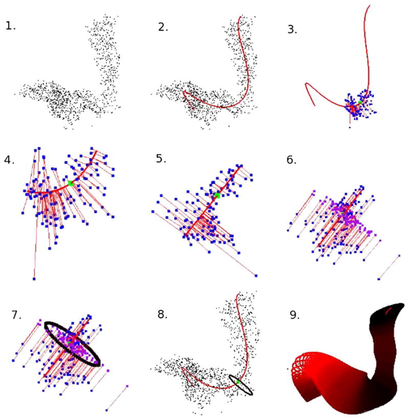
A “Roadmap” of the tube-fitting algorithm.

The curve fitted through the center of the data represents the “spine” of the tube. It is also useful in our applications to represent the metric by which measures of extent of the tube are taken. This component relies on existing methodology; the remaining steps of the tube-fitting algorithm and the application to two imaging modalities represent the methodological advances of this manuscript.

We apply the tube-fitting algorithm to an example of each type of image. The results indicate that the procedure could be used in the SPECT application as a replacement for the invasive sigmoidoscope procedure, which is currently used instead of image processing. In the second application, our algorithm is used to extract MRI quantities at many points along a white-matter tract. This is an improvement over the current approach, which examines tracts by looking at a sequence of axial slices along the image and which does not produce satisfactory results when the long axis of the tube is not normal to the axial plane (see Section 6).

The manuscript is structured as follows. Section 2 describes the data sets in detail. Section 3 outlines the modified-principal-curve algorithm that serves as the basis of the tube-fitting procedure. Section 4 gives the detailed tube-fitting algorithm. Section 5 provides a validation study of the algorithm. Section 6 presents the application to SPECT and DT images. Section 7 is a discussion.

2. Motivating data sets

2.1. SPECT colon imaging

Our SPECT colon data arise from an experiment designed to study the viability of microbicide lubricant for HIV transmission during anal intercourse [Hendrix et al. (2008); Hendrix, Cao and Fuchs (2009)]. SPECT imaging uses a radioactive isotope as the source signal. Projections of emitted photons are collected via gamma cameras mounted on a gantry that are rotated around the subject. Computed tomography algorithms are used to convert the projection images into a three-dimensional image. The principal benefit of SPECT imaging is the ability to image changes in tracer position and distribution within an anatomical structure over time, rather than simply imaging anatomy.

The experiment was designed to simultaneously image the distribution of surrogates for the microbicide lubricant and the viral-mixed semen to assess if the coverage of the lubricant is sufficient. The experiment used an over-the-counter lubricant as a surrogate for the microbicide, which was mixed with a radioactive tracer (TC-sulfur colloid). A radiolabeled surrogate for the viral-mixed semen is being used for extensions of the experiment, though the data considered here contains only the lubricant.

Ten milliliters of the radiolabeled lubricant was injected into the subject’s colon, who subsequently simulated receptive anal intercourse using an artificial phallus. The subject was then imaged using a dual-head VG SPECT imaging system (GE Medical Systems, Waukesha, WI) equipped with a low-end X-ray computed tomography system (Hawkeye). The image was reconstructed using an ordered subsets EM algorithm and filtered as provided with the scanner software (GE eNTE-GRA workstation, version 1.04). We present analysis of the reconstructed SPECT image of the distributed lubricant.

2.2. Quantification of DTI tractography

As mentioned above, DTI [Basser, Mattiello and LeBihan (1994b)] has two major values as an imaging modality: its sensitivity to tissue microstructure [Beaulieu (2002)] and its ability to guide tractography of the major white matter tracts [Mori et al. (1999)]. This is due to DTI’s sensitivity to diffusion anisotropy [Basser and Pierpaoli (1996)]—the tendency of water to diffuse in a particular direction, which, in the brain and spinal cord, is often along the course of an axonal tract. By combining analysis of tissue microstructure with tractography, we can limit our focus to one or several tracts with specific functional correlates, for example, motion, vision and language. Within these tracts, we can analyze not only quantities derived from DTI including anisotropy, absolute and directional diffusivity of water, and tract volume, but also quantities derived from other MRI sequences that have been coregistered to the DTI [Reich et al. (2007)]. This offers the possibility of a comprehensive, multimodal approach to analyzing the structure-dysfunction relationship in the central nervous system.

To compare tract-specific imaging results across individuals, a normalization procedure is required. There are two general approaches: whole-brain normalization, which involves warping brains to match one another or some canonical atlas, and tract-specific normalization, which focuses specifically on the tract of interest. The former approach is computationally intensive and may require sacrificing optimal registration of the tract of interest to achieve acceptable registration of the whole brain. We have introduced an approximate tract-specific normalization approach that samples tracts in a slice-by-slice manner [Reich et al. (2007)]; this approach has yielded promising correlations between tract-specific MRI quantities and clinical disability scores [Reich et al. (2008, 2009)]. However, because white matter tracts in the brain do not typically run perpendicular to the cardinal imaging planes (axial, coronal and sagittal), a parametric approach that accounts for each tract’s specific shape and anatomical course would reduce noise and might increase sensitivity for detection of relevant abnormalities. The parameterization would be different for each tract but would ideally be generated by an algorithm that could be applied automatically to any tract. In particular, we hope that the tube-fitting algorithm will allow us to estimate quantities derived from DTI at many points along a tract, regardless of the anatomical course of that tract.

Details of our MRI acquisition protocol have been described [Reich et al. (2006)]. On a 3-Tesla Philips Intera scanner, we obtained whole-brain DTI images in the axial plane (2.2 × 2.2 × 2.2 mm voxels interpolated on the scanner to 0.8 × 0.8 × 2.2 mm; parallel imaging with a sensitivity-encoding reduction factor of 2; 2 averages; 32 noncoplanar gradient directions with a nominal b-value of 700 s/mm²; and a scanner average of 5 minimally diffusion-weighted scans with b ≈ 33 s/mm²). We coregistered all images to the first minimally diffusion-weighted scan using the Automatic Image Registration (AIR) algorithm [Woods, Cherry and Mazziotta (1992)] with a 6-parameter rigid-body transformation, and we corrected the gradient directions for the rotational component of the transformation. We then estimated the diffusion tensor in the standard fashion [Basser, Mattiello and LeBihan (1994a)], diagonalized the tensor to obtain its eigenvalues and eigenvectors, and calculated maps of anisotropy and diffusivity. These analyses were performed in DtiStudio [Jiang et al. (2006)], as well as with custom software purpose-written in Matlab (The Mathworks, Natick, MA).

We used the DTI data sets to obtain 3D reconstructions of the corticospinal tracts using the fiber association by continuous tractography method [Mori et al. (1999, 2005); Mori and van Zijl (2002)]. We reconstructed the tracts using fractional anisotropy and the principal eigenvector of the diffusion tensor. We used every voxel in the brain with fractional anisotropy > 0.13 as a potential starting point for tractography and halted individual tracts once a voxel with fractional anisotropy < 0.13 was encountered or when the reconstructed tract turned at an angle steeper than 40 degrees from one voxel to the next. We chose multiple restrictive regions of interest to limit the reconstructed corticospinal tracts to their known anatomical course; these regions of interest have been described previously [Reich et al. (2006)] and were drawn in the rostral medulla, rostral pons and subcortical white matter. We manually excluded the rare spurious fibers that were included in this reconstruction but that clearly fell outside the major portion of the corticospinal tract.

3. Modified principal curve algorithm

To construct our tube, we first need a fitted curve that acts as a centerline for our data. Statistical analysis for three-dimensional curve-fitting and centerline calculation has received little attention in the statistical community. (We emphasize the difference between fitting nonparametric functions, a process well studied in the smoothing literature, and nonparametric curve-fitting.) However, curve fitting has received a great deal of attention in the computer-vision and medical-image-processing literature. Relevant literature exists in the field of virtual colonoscopy and localization of polyps [see, for example, McFarland et al. (1997); Samara et al. (1998, 1999); Hong et al. (1997); Chiou et al. (1998); Deschamps and Cohen (2001)]. These approaches generally require connected curves, and are not directly applicable to the range of problems that we consider, which may have interrupted structures or may be a voxel-wise reduction of connected-curve data. Also relevant from the image processing literature is the tremendous volume of work on Bezier curves and B-splines [see the review in Cohen, Riesenfeld and Elber (2001)]. Though we have explored Bezier approaches, we do not utilize them because of the large amount of user input required to appropriately place knots.

Another popular collection of techniques treats the points of the image as a networked graph and uses combinatorial algorithms to find globally optimal paths [Cohen and Kimmel (1997); Chaudhuri et al. (2004); Chiou et al. (1999); Bitter et al. (2000a, 2000b)]. Dijkstra’s algorithm is often used to find solutions [Dijkstra (1959)].

Perhaps the most statistical approach that we have encountered relies on the use of principal curves [Hastie and Stuetzle (1989); Hastie (1984); Hastie, Tibshirani and Friedman (2001)]. These generalizations of principal components find a curve achieving a local minimum for the sum of the orthogonal distances of the points onto the curve. This approach is useful in statistical methods of image analysis [Banfield and Raftery (1992); Caffo et al. (2009)]. Numerous modifications of the principal-curve idea have been published [see the discussion in Kegl et al. (2000)]. In addition, there are related stochastic search algorithms for finding centerlines, as considered in Deng (2007). Our approach in this manuscript utilizes the modified-principal-curve algorithm presented in Caffo et al. (2009). This procedure can accommodate interrupted curves, constrained points and can fit low variation curves that the original algorithm could not. We briefly describe the procedure below.

To start, we need a method for representing a curve. The study of differential geometry has revealed several equivalent methods for representing real-valued curves [Cohen, Riesenfeld and Elber (2001); Thorpe (1979); Kreyszig (1991)], including implicit representations, the set of points {(x, y, z) ℝ³ | F (x, y, z) = G(x, y, z) = 0}, for surfaces F and G and parametric representations. We focus entirely on parametric representations, of which implicit representations are a special case [Kreyszig (1991)]. An allowable parametric representation sets f (t) = {f^x(t), f ^y(t), f ^Z(t)}: [a, b] → ℝ³, where [a, b] is an interval in ℝ and at least one of df ^x(t)/dt, df ^y(t)/dt or df ^z(t)/dt is nonzero. We assume the constraint t ∈ [0, 1] for identifiability. However, this assumption alone does not uniquely specify a curve. Indeed, if the curve is considered to be the location of a particle at time t, then the same curve can arise from particles following the same path at different rates.

Given this parametric curve representation, we view the process of fitting a curve through three-dimensional coordinates as inherently a missing-data problem. Let ${\{(X_i,Y_i,Z_i)\}}_{i=1}^n$ be a collection of realized values for the coordinate functions. The process of finding a curve through them largely amounts to finding a reasonable estimates for the missing data ${\{t_i\}}_{i=1}^n$. However, estimating the missing time data, ${\{t_i\}}_{i=1}^n$, is a difficult process.

Here ${\{X_i,Y_i,Z_i\}}_{i=1}^n$ are lattice values of points in the image surviving a thresholding procedure for noise reduction. In addition, to improve computing times, we often work with a subset of the points, sampled uniformly, as the curve is often well defined with much fewer points. This is not necessary for the DTI tractography example, but it speeds up computing substantially at no loss of quality-of-fit for the SPECT colon data.

The basic principal curve algorithm is a blocked-maximization algorithm that iterates between two steps: calculating the time points and fitting curves to the coordinate data: {(X_i, t_i)}, {(Y_i, t_i)}, {(Z_i, t_i)}. Suppose that an initial estimate of f, say, f̃, is given. Then, the t_i are calculated as

$$t_i=\underset{t\in [0,1]}{\text{argmin}}\left|\right|\stackrel{\sim }{f}(t)-(X_i,Y_i,Z_i)\left|\right|.$$ (1)

The estimate f̃ is then updated by fitting a smoother between the {X_i} and the {t_i}, the {Y_i} and the {t_i}, and the {Z_i} and the {t_i}, separately. We use cubic regression splines for this portion of the algorithm, though other smoothers could be used. However, regression splines allow for easily calculated derivatives on the coordinate function. The steps of updating the {t_i} and f̃ are iterated until the change in f̃ between successive steps is sufficiently small.

Several modifications to the principal curve algorithm outlined above are proposed by Caffo et al. (2009). First, the modified-principal-curve approach allows for user-specified end points. Second, it molds the curve by gradually increasing the degrees of freedom in the regression splines, so that gross features of the curve are captured before fitting finer details. This provides for better fits to complex curves. Third, the modified approach incorporates image intensities to adjust the emphasis placed on high- and low-intensity points in the curve-fitting. Fourth, a grid search is used to perform the minimization in the second step of the algorithm to speed up convergence. Finally, the stopping criterion is based on relative change in mean square error. As described originally, the modified-principal-curve-fitting algorithm also allows for user-specified interior points, though constrained interior points did not lead to better fits in our applications.

The modified principal curve algorithm is semiautomated, requiring user defined endpoints and, in some cases, adjustment of the final number of degrees of freedom used in the regression splines. This algorithm provides a differentiable curve that acts as a centerline through the data. We emphasize, however, that the algorithm used to construct the centerline curve functions independently of the algorithm used to fit the tube. So, for example, other less automated procedures, such as using B-splines with user-selected knot points, could be used for this step.

4. Tube-fitting algorithm

In the previous section we outlined the curve-fitting algorithm, which provides the centerline for our tube-fitting algorithm. Before we begin the exposition of the tube-fitting algorithm, we pause briefly to reiterate our goal and outline our general approach.

In this section our aim is to provide an estimate of the boundary of a tube-shaped structure based on a collection of observed data points from the interior of this structure. To accomplish this, we estimate the centerline of the structure and, at many points along this centerline, estimate the cross-sectional extent of the tube. The tube-fitting algorithm consists of a collection of steps that can proceed from any point on the centerline and progresses to an estimate of cross-sectional boundary of the tube. While the basic outline of the procedure is simple and intuitive, many of the steps require special care.

The steps in the tube-fitting algorithm are as follows: (i) select a starting point f₀ on the centerline; (ii) identify nearby image points; (iii) project nearby image points onto the plane orthogonal to the centerline at f₀; (iv) fit a bivariate normal distribution to the (now two-dimensional) points in the orthogonal plane; (v) use a level set of the bivariate normal to define the tube at the chosen starting point on the fitted curve. Each of these steps will be examined in greater detail in the following subsections. Further, we encourage the reader to refer often to Figure 1, which shows graphically the steps in the tube-fitting algorithm.

We pause to discuss the choice of an ellipse (the level set of a bivariate normal) as the shape of the cross-sectional boundary of the tube. Our first inclination was to use the convex hull—the smallest closed set containing the points—because it is flexible and comparatively unrestrictive. For a one-dimensional cross section, this approach is analogous to using the minimum and maximum. However, such estimates do not account for any noise in the measurements inherent in some imaging techniques and would only be acceptable for very high resolution images without noise. Moreover, similar to elliptical cross sections, convex hulls cannot estimate nonconvex cross-sectional shapes. A circle centered at the origin, that is, the level set of a bivariate normal distribution with no correlation, was too restrictive for the shapes seen in practice.

Therefore, as a compromise between these extremes, we use an ellipse to define the boundary of the tube. This choice coincides with observed points projected into the orthogonal plane as well as our scientific collaborators’ knowledge of the anatomical structures in our motivating data sets; for other applications, a different choice for the shape of the boundary may be needed. We emphasize that our algorithm is easily adapted to these other applications, in that only the final step is changed. Last, in Section 4.7 we explore our algorithm’s performance in a case in which the cross section is not elliptical.

4.1. Step 1: Selecting a starting point

The elements of the tube-fitting algorithm discussed in this subsection are illustrated in panels 3 and 4 of Figure 1.

As noted, the tube-fitting algorithm consists of several steps that are repeated along the length of the centerline. We prefer to take 50 equally spaced points on the centerline as the individual starting points at which we estimate cross sections of the tube. The steps in the algorithm are the same, regardless of the position of the starting point. To aid in the clarity of our figures, we display a starting point in the middle of the curve. We emphasize that the starting points, and hence the locations where the cross section of the tube is estimated, do not have to be the projection of an observed point onto the curve, nor does it have to lie on the lattice defined by the imaging coordinates.

Notationally, we will call the starting point on the centerline f₀. Also, we recall the latent variable t that was used in Section 3 to parameterize the centerline f (t). Let t₀ be the value of that variable such that f₀ = f (t₀). The variable t will prove to be a useful tool in the following steps, as it orders the image points according to their orthogonal projection onto the centerline f (t).

4.2. Step 2: Identifying nearby image points

The elements of the tube-fitting algorithm discussed in this subsection are illustrated in panels 3 and 4 of Figure 1.

Again, in the steps of our algorithm we are trying to estimate the cross-sectional extent of the tube-shaped structure at f₀. We base our estimate of the boundary on image points that are local to f₀. In this subsection we discuss what is meant by “local” in this context.

Let the set ${\{P_i\}}_{i=1}^n$ be the points from the image used in the curve-fitting procedure, so that P_i = (X_i, Y_i, Z_i). Recall that in Section 3 we assigned to each P_i a value of the latent variable t_i such that the distance between P_i and the centerline f (t) is minimized. Our goal in this subsection is to select points in ${\{P_i\}}_{i=1}^n$ that are near f₀. We use the collection ${\{t_i\}}_{i=1}^n$ to do this. As we argue below, this is preferable to the seemingly more intuitive approach of using Euclidean distance.

The neighborhood of points to be used in estimating the cross-sectional extent of the tube is

$$\{P_{i_j}\}=\{P_i\mid \mid t_0-t_i\mid <t_r\},$$ (2)

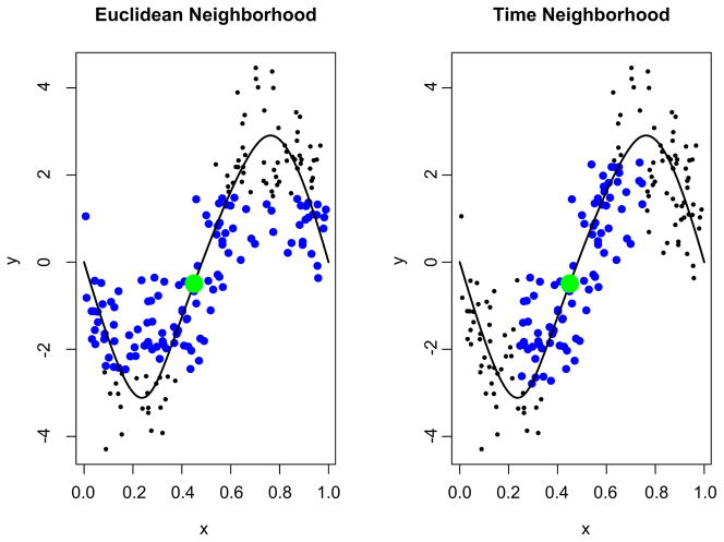
where t_r is the range of the time window. Intuitively, measuring proximity in terms of the latent variable t allows us to select the nearest neighbors of f₀, defining “local” in terms of distance on the curve f (t). This strategy for defining a neighborhood of observed points around f₀ has major benefits over competing methods, such as using a neighborhood based on the Euclidean distance between the observed points and f₀. Specifically, for f₀ near high curvature in the fitted curve, observed points can then overly contribute to the fitted tube at multiple locations. See Figure 2 for a two-dimensional illustration. The blue points in the left panel are in the Euclidean neighborhood structure of P₀, and include points that lack face validity for contributing to the estimate of the extent of the tube. In contrast, the right panel shows that the neighborhood defined as (2) has much better behavior. We note that in areas of low curvature, our method for choosing {P_ij} coincides with the method using Euclidean distance.

Fig. 2.

Comparison of methods for defining the neighborhood around f₀. In the left, the neighborhood is defined as though points with a Euclidean distance from f₀ less than 2; in the right, we use a t-window with t_r = 0.2. In both, the point f₀ is shown in green, and the points in the set {P_ij} are shown in blue.

For our applications, we have found that choosing 0.05 ≤ t_r ≤ 0.2, depending on the total number of image points, includes enough points to estimate the tube’s shape without using locations that are very distant. (Recall that our curve-fitting algorithm specifies 0 ≤ t ≤ 1.) However, we emphasize that truncating points in this way is done primarily for computational purposes. In estimating the extend of the tube, we weight points (see below) by their distance in t, so that further away points contribute less to the estimate.

4.3. Step 3: Local linearization and projection onto the cross-sectional plane

The elements of the tube-fitting algorithm discussed in this subsection are illustrated in panels 5 and 6 of Figure 1.

Thus far, we have selected a starting point f₀ and found the collection of nearby points {P_ij}. Next, we will project the points {P_ij} onto the orthogonal cross section; once the points are projected into a single two-dimensional plane, we will estimate the tube’s extent.

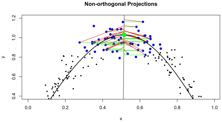
The projection of the set {P_ij} onto the orthogonal plane is a step that may strike a reader as unexpectedly complex. A simple, intuitive and standard approach is to take as the projection of P_i the point in the orthogonal plane with minimum Euclidean distance from P_i. However, in the context of our tube-fitting algorithm, this standard projection fails in the following way. In areas of modest or high curvature, such projections skew toward the interior of the curve, rather than remaining centered around the centerline. Estimates of the extent of the tube are therefore similarly skewed. Figure 3 illustrates this point using a two-dimensional analog, showing standard projections and projections using our novel projection approach which we explain next. A three-dimensional illustration appears in Section 5.

Fig. 3.

Two projection methods shown in an area of high curvature: in green, standard projections minimizing the distance between a point and the line; in red, our modified projections that maintain a point’s distance from the fitted curve. Again, f₀ is highlighted in green and the {P_ij} are shown in blue.

Instead of the standard projection, we use a method that maintains a point’s distance and direction from the centerline in its projected position on the orthogonal plane. Conceptually, our method stretches the space containing the centerline f (t) and the points P_i around it so that f (t) is linear. Our conceptual framework then considers the plane containing the image point P_ij and the point on the centerline f (t_ij) as a transparent sheet [note this plane is orthogonal to the centerline at f (t_ij) from our construction of t_ij]. The projection of {P_ij} onto the cross-sectional plane is found by stacking one such transparent sheet for each point in {P_ij}, overlaying them so that the points {f (t_ij)} coincide.

More technically, our projection method is carried out in the following steps. Consider the plane orthogonal to f (t_i). By the construction of f (t), both P_i and f (t_i) lie in this plane. We rotate and translate this plane so that: (i) the plane is parallel to the axial plane of the image (i.e., is horizontal), (ii) the height of the plane is Z = 0, and (iii) the point f (t_i) is at the origin.

To accomplish this, we let n = g(t_i) = ▽ f (t_i)/||f (t_i)|| and, hence, the plane orthogonal to f (t) at f (t_i) is the collection of points R = {r ∈ ℝ³ | n · (f (t_i) − r) = 0}. Let A be the rotation matrix so that AR is horizontal (parallel to the XY plane). Finally, let $P_i^{\prime }=\mathbf{A}{\mathbf{P}}_{\mathbf{i}}-\mathbf{A}f(t_i)$.

Notice that $P_i^{\prime }$ has Z coordinate 0 and its distance from the origin is equal to the distance between P_i and its projection onto the fitted curve, f (t_i). We perform this process for all points in the neighborhood of P₀, {P_ij}, to obtain a set of rotated and translated points, { $P_{i_j}^{\prime }$}. These points in two-dimensional space have distance and direction from the origin that is the same as their distance and direction from the fitted centerline. In effect, we have locally linearized our fitted curve and collapsed the locations in the current t -window into a single plane.

4.4. Step 4: Fitting a bivariate normal in the orthogonal plane

In Sections 4.1 and 4.2 we selected a starting point and found image points that were near our starting point. In the previous section we projected points local to f₀ onto the cross-sectional plane. Next, we fit a bivariate normal distribution to the projected points in the cross-sectional plane.

Our task here is subtly affected by our overarching goal to provide an estimate of the boundary of the tube-shaped structure at our current starting point f₀. While we have selected points local to f₀ to construct this estimate, we further use weights so that more distant points have a smaller impact on the estimation than nearer points. Again, we use the latent variable t as a tool for constructing these weights, precisely because t is a measure of distance along the centerline rather than a measure of Euclidean distance.

Specifically, we use a cosine-transformed distance as the weight:

$$w_{i_j}=\frac{cos[(t_{i_j}-t_0)\pi /r]+1}{{\sum }_{j=1}^{J}cos[(t_{i_j}-t_0)\pi /r]+1}$$ (3)

with r the half width of the t-window. This weighting scheme has the desired effect of emphasizing nearby points while smoothly decreasing to zero for more distant points. We note that other weighting schemes that decrease to zero at the tails, specifically kernel weighting schemes, give very similar results. Schemes that do not decrease to zero, like one that gives uniform weight to all points in the t window, are less desirable because the resulting tube is not necessarily smooth.

Let {w_ij} be the collection of normalized weights. Then the estimated bivariate normal has mean and variance

$$\stackrel{\sim }{\mu }=\sum _{j=1}^J{w}_{i_j}{P}_{i_j}^{\prime }\text{and}\mathrm{\sum }^{\sim }=\sum _{j=1}^J{w}_{i_j}(P_{i_j}^{\prime }-\stackrel{\sim }{\mu }){(P_{i_j}^{\prime }-\stackrel{\sim }{\mu })}^T,$$ (4)

where 1 ≤ j ≤ J indexes i_j and { $P_{i_j}^{\prime }$} is the projection of the local points into the cross-sectional plane.

4.5. Step 5: Estimating the tube’s boundary

The elements of the tube-fitting algorithm discussed in this subsection are illustrated in panels 7 and 8 of Figure 1.

In the final step of our algorithm, we select a level set of the bivariate normal fit in the previous step as our estimate of the cross-sectional boundary of the tube. In the two-dimensional cross-sectional plane, the tube is estimated by the level set

$${\widehat{G}}^{\prime }(t_0)=\{P\in {\mathbb{R}}^2\mid \mid 2\pi \mathrm{\sum }^{\sim }{\mid }^{-1/2}exp\{-{(P-\stackrel{\sim }{\mu })}^{\prime }{\mathrm{\sum }^{\sim }}^{-1}(P-\stackrel{\sim }{\mu })/2\}>l\},$$ (5)

where Ĝ (t₀) is the elliptical estimate of the boundary and l is chosen so that

$${\int }_{P\in {\widehat{G}}^{\prime }(t_0)}\mid 2\stackrel{\sim }{\pi }\mathrm{\sum }^{\sim }{\mid }^{-1/2}exp\{-{(P-\stackrel{\sim }{\mu })}^{\prime }{\mathrm{\sum }^{\sim }}^{-1}(P-\stackrel{\sim }{\mu })/2\}dP=1-\alpha .$$ (6)

Typically the choice of α will be context-specific, depending on the shape of the true boundary G(t₀) and the measurement error variance (if any exists). In Section 4.6 we explore the effect of α on the resulting estimate Ĝ (t₀). Last, we recall that our projection method took each point into the XY -plane through a series of rotations and translations. We apply these steps in reverse to take the fitted ellipse into our original space.

4.6. Choosing α

As previously mentioned, the underlying modality and noise characteristics of the image impacts how one selects the cross-sectional ellipse covering the structure; in other words, how one selects α in the level set of the bivariate normal. Our two examples highlight the difficulty in obtaining a universal rule. The SPECT image is clearly very noisy, as is required by the underlying Poisson decay of the tracer and the other sources of noise imposed during image acquisition and reconstruction. The DTI tract, on the other hand, appears nearly noise free. However, there is noise in the underlying DTI image and potential noise and bias from the tractography algorithm. However, without repeat scans, it is impossible to characterize this variability in the DTI image. Therefore, we seek the most accurate representation of the tract image, acknowledging that there are sources of noise and bias that are not represented or quantified. Thus, the choice of α differs greatly in these two applications.

To elaborate on this choice, we have two competing goals: (i) to maximize the coverage of the true cross section by our estimated ellipse; and (ii) to avoid choosing the ellipse excessively large through the inclusion of points not in the cross section. To characterize these goals, we examine the quantities

$$TP=\frac{A\{G(t_0)\cap \widehat{G}(t_0)\}}{A\{G(t_0)\}}\text{and}FP=\frac{A\{G{(t_0)}^c\cap \widehat{G}(t_0)\}}{A\{G(t_0)\}},$$ (7)

where A(·) gives the area of the designated shape, and again G(t₀) is the true cross-sectional boundary of the tube and Ĝ (t₀) is the elliptical estimate of the boundary. These quantities, TP and FP, can be thought of respectively as the true and false positive rates normalized to the area of G(t₀), so that 0 ≤ TP ≤ 1 and 0 ≤ FP. These quantities are analogs of the true and false positive rates from the analysis of classification data.

As discussed above, because it depends highly on the distribution of measurement errors and other factors, the choice of α will be context-specific. We therefore advise a validation study tailored to the application at hand, if such a study is possible. Indeed, in Section 5 we present validation data both to confirm the tube-fitting algorithm and to aid in selecting α for our SPECT imaging application. However, a study of this kind is not always possible, so here we present a brief simulation designed to provide a basis for evaluating the interplay between the choice of α and noise levels in the image.

We posit an underlying collection of true points from an ellipse and add spherical noise. The goal is to estimate the ellipse. Thus, two sources of variation are considered, the sampling of underlying true points and noise. The simulation consisted of the following steps:

1. Points are sampled uniformly from the interior of the underlying ellipse G.

2. Normal errors with variance matrix Σ = σ²I_2×2 are added to the sampled points to give observed points.

3. From the observed points, a bivariate normal is estimated and used to construct Ĝ for a range of α values.

4. TP and FP are calculated for each of the α values.

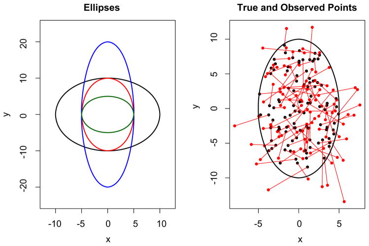
These steps are iterated 100 times each for a variety of ellipse shapes and measurement error variances. Figure 4 shows some of the ellipses G used in our simulation, as well as a representative collection of sample points and observed points.

Fig. 4.

The left panel shows several of the true ellipses used in our simulation. On the right, we show the points sampled uniformly from an ellipse in black and the points observed with measurement error in red.

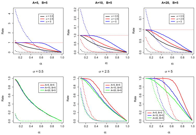
We found that two main factors should contribute to the choice of α: the measurement error variance and the eccentricity of the ellipse. The eccentricity of an ellipse with semi-major and -minor axes A and B, respectively, is defined as $e=\sqrt{\frac{A^2-B^2}{A^2}}$. For low measurement error variance, say, σ = 0.1 * B, the eccentricity of the ellipse is irrelevant: taking α = 0.12 gives TP = 0.95 and FP = 0.1. For large measurement error variance, the eccentricity of the ellipse is quite important. Indeed, for an ellipse with A = B and σ = B, α = 0.62 yields TP = 0.95 and FP = 0.2, while for an ellipse with A = 4B and σ = B, the same choice of α gives TP = 0.55 and FP = 0.05. Figure 5 shows the results of our simulation study. We present these results in two ways. First, keeping the eccentricity of the ellipse constant, we examine the effect of varying σ on TP and FP. Second, we keep σ constant and allow the shape of the ellipse to vary. Finally, we note that the results presented here hold for ellipses in other scales; that is, TP and FP as a function of α are the same for A = B = 10 and σ = 5 and for A = B = 100 and σ = 50.

Fig. 5.

Results of the simulation for choosing α. For all panels, the solid line represents TP and the dashed line FP. In the top row, each panel fixes the shape of G and varies σ, while in the bottom row σ is fixed for each panel and the shape of the ellipse changes.

4.7. Performance of ellipse as cross-sectional shape

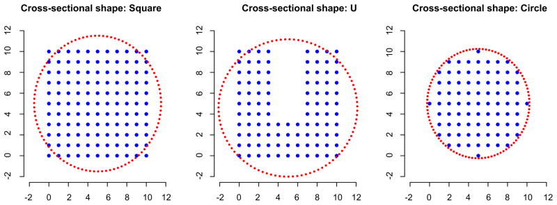
Finally, we used a simulation study to examine the effect of choosing an ellipse as the shape for the tube’s cross section when the true cross section is nonelliptical. We used a variety of cross-sectional shapes: a square, a “U” and, for reference, a circle. For each cross section, we created a three-dimensional structure by stacking fifty copies of the shape, one on top of the next. We applied the tube-fitting algorithm as presented (that is, using an ellipse as the cross section) with α = 0.12 to each of these structures.

In Figure 6, we show each of the cross sections, as well as a typical estimated ellipse. For the square, our ellipse misses the corners and mistakenly includes extra points on the sides. However, the true and false positive rates, 0.967 and 0.146, respectively, indicate that miss-specifying the cross-sectional shape in this case still provides a reasonable estimate of the three-dimensional structure. We note that using a convex hull as to estimate the extent of this structure would be ideal, having a true positive rate equal to 1 and a false positive rate equal to zero. For the “U” shape, the ellipse includes almost all of the true image points, but also includes a large number of nonimage points; the true and false positive rates are 0.98 and 0.338. This cross-sectional shape is particularly difficult; a convex hull would include many nonimage points and have a high false positive rate. For the circle, the ellipse performs well, as is expected; the true and false positive rates are 1 and 0.089. Further, we note that taking α = 0.14, rather than α = 0.12, gives true and false positive rates equal to 1 and 0, respectively.

Fig. 6.

Three true cross-sectional shapes used in our simulation, as well as a typical estimated ellipse.

From this simulation, we see that misspecification of the cross-sectional shape can result in a lower true positive rate and higher false positive rate, but that the performance of the fitted tube is generally still reasonable. Moreover, in situations where the true cross section is approximately or exactly elliptical, as is true in our applications, the fitted tube performs quite well. Last, we reiterate that the choice of the cross-sectional shape is the last step of the tube-fitting algorithm, and can be changed in a straightforward way in other applications without affecting the majority of the algorithm.

5. Validation

Before applying our tube-fitting algorithm to image data, we pursued a brief validation study using mathematical phantoms. A mathematical phantom is simply a shape, created digitally, which is then passed through a computational model of the imaging process. Accurate computational models of diffusion imaging are not available due to the inherent complexity of nuclear spin systems and water diffusion. On the other hand, very accurate models for some transmission and emission imaging, such as X-rays, planar scintigraphy, SPECT, PET (positron emission tomography) and CT (X-ray computed tomography) are available. In these cases the imaging process is perhaps simpler to model than in MRI and highly accurate models of the imaging physics have been created. To generate the SPECT images for validation, we used system models implemented in the Division of Medical Imaging Physics in the Department of Radiology at the Johns Hopkins University. In this method, the projection data of the phantom were obtained using an analytical projector that models all of the important components of the images physics, including photon interactions inside both the phantom and the detector system. The 3D SPECT images were then reconstructed from the projection data using an iterative statistical algorithm.

Our phantom is a three-dimensional coil of fixed diameter; we also investigated coils with monotonically increasing or decreasing diameters, with very similar results. The phantom was projected using the analytical projector described above with effects of attenuation and detector resolution blur. Poisson noise with data-derived means was also added to the projection data. Several noise levels were investigated to mimic images taken at baseline, three hours, 10 and 24 hours after introduction of the tracer. (Later images are noisier than earlier images.) The SPECT images were reconstructed using the OS-EM algorithm [Hudson and Larkin (1994)].

Each image had an imaging space of over 20,000 nonbackground voxels. To speed up curve-fitting and tube-fitting algorithms, we randomly sampled 1000 locations among these, separately for each validation image. The algorithms were run on the sampled locations, and the resulting fitted tube was compared to the true underlying anatomical structure. Additionally, we varied the level set of the bivariate normal used to define the tube at each point along the fitted curve, which is equivalent to varying the choice of α. Particularly, we were interested in the proportion of points included in the tube that were indeed in the anatomical structure (true positives), the proportion of points included in the tube that are not in the structure (false positives), and the effect of α—the level of the bivariate normal used in constructing Ĝ ′ (t₀)—on these rates. Our goals are to maximize the true positive rate while minimizing the false positive rate; that is, we want our tube to be large enough to capture the structure but not so large as to include extraneous points.

There are two important differences between our current validation study and the simulation study in Section 4.6. The first is that our current study is tailored to the SPECT application, and is therefore preferable for selecting α in this setting. Second, the true and false positive rates discussed here are taken over the entire fitted tube, rather than at a single fitted ellipse as in our previous simulations.

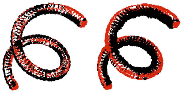
It is worth noting that the fitted tube captured the shape of the anatomical structure quite well, even in noisier images. As seen in the left panel of Figure 7, the false positives and false negatives occurred primarily in a thin layer on the outer surface of the anatomical structure. These errors are at least in part due to variations in the fitted curve and tube induced by randomly sampling 1000 points from the more that 20,000 nonbackground voxels rather than to a general deficiency in the tube-fitting algorithm. All other errors occurred at the endpoints of the tube, due to the placement of the user specified endpoints in the the curve-fitting algorithm. We include in the right panel of Figure 7 a similar image for a tube constructed using standard orthogonal projections. Here, the false positives occur almost exclusively on the interior side of the structure and the false negatives occur almost exclusively on the exterior side; this is consistent with our concerns above, namely, that orthogonal projections skew toward the interior of the fitted curve. These observations reinforce our projection method and give us confidence in the ability of the tube-fitting algorithm to accurately reproduce an imaged structure.

Fig. 7.

False positives (black) and false negatives (red) in tubes fitted to a SPECT scan at 10 hours. Tubes were constructed using our local linearization method of projecting (left) and standard orthogonal projections (right).

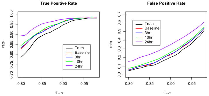
Figure 8 shows the true and false positive rates as a function of 1 − α. From these graphs we see that for a fixed α, noisier images contain greater rates of both true and false positives; the noise in the image leads to a wider fitted tube. We also note that the α level set used to construct the tube does not correspond to the true positive rate. Hence, it must be viewed as a tuning parameter used to balance the true and false positive rates. Based on these figures, we select 0.8 ≤ 1 − α ≤ 0.9, depending on the amount of noise in the image. For noiseless images (shown in Figure 8 as “Truth”), choosing 1 − α = 0.9 gives a true positive rate ≈0.95 and a false positive rate ≈0.15; for our noisiest image (24 hours after baseline), choosing 1 − α = 0.8 gives similar rates. We note that our selection is based on visual inspection rather than a well-defined optimizing procedure.

Fig. 8.

True positive and false negative rates for each of the five validation images as a function of the level used to determine the fitted tube.

6. Applications

6.1. SPECT images

We first consider the SPECT colon image, which was taken shortly after introduction of the tracer. We first filtered the image with a simple histogram filter to remove low intensity background noise and artifacts from the reconstruction process. Next we sampled a subset of the remaining points to both fit the curve and the tube. We used the modified principal curve-fitting algorithm with K = 5 final degrees of freedom to find the centerline. Next, we employed the tube-fitting algorithm with a time window width r = 0.2 and α = 0.15. Other time windows produced generally similar results. However, shorter windows are more sensitive to local variations in the density of sampled points, whereas longer windows oversmooth and lose some gross anatomical features.

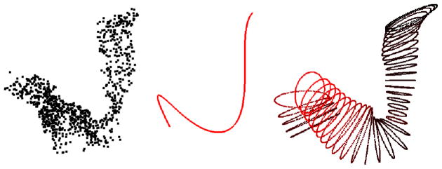
Figure 9 shows the sampled colon data, the fitted curve and the fitted tube colored according to tracer concentration. As described above, the tracer concentration at each point along the curve was taken to be the summed concentration of those points used to define the tube at that point. Though the fitted tube plausibly recreates colon anatomy in terms of shape and width, we are unable to make a comparison between the fitted tube and the subject’s colon. SPECT-CT scanners typically produce poor CT scans; therefore, we lack good anatomical images that could be used to make this comparison. However, a benefit of the tube-fitting method is that it allows us to recreate the colon without radiating participants unnecessarily or requiring additional expensive equipment.

Fig. 9.

Three steps of the tube-fitting process. Farthest left is the sampled data from the SPECT image; center is the centerline produced by the curve-fitting algorithm; right is the fitted tube, shaded by tracer concentration (red is higher concentration, black is lower).

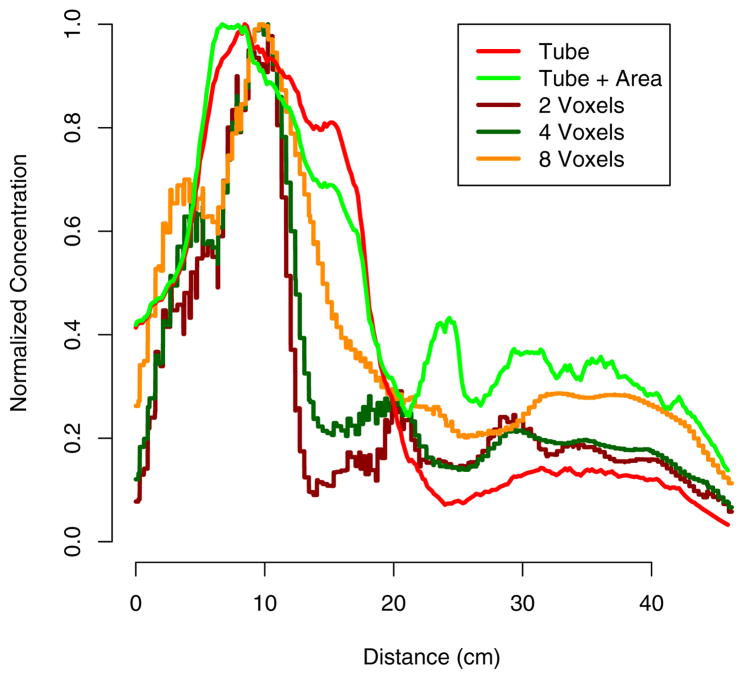
Figure 10 shows the concentration-by-distance curve. To find distance along the curve, we initially employed the arc-length formula

Fig. 10.

Concentration by distance from beginning of curve (near the anus). Concentration calculated using t-window and voxel-neighborhood approaches. Each curve is normalized to its maximum value.

$$d(t)={\int }_0^T\sqrt{{\left\{\frac{d}{dt}{\widehat{f}}^x(t)\right\}}^2+{\left\{\frac{d}{dt}{\widehat{f}}^y(t)\right\}}^2+{\left\{\frac{d}{dt}{\widehat{f}}^z(t)\right\}}^2}dt,$$ (8)

using the final fitted curve. Though often the gradient of the fitted curve is easy to calculate, a closed-form solution for the integral is not available. We have found that simply calculating distance using the function value along the fine grid of values of t used to create the tube is equally accurate. That is, we simply use linear approximation between equally spaced latent time points to measure distance along the curve.

Computing the concentration at each distance from the curve onset can be accomplished in a variety of ways. Using the the neighborhood of t₀ described in Section 4, we can define for each ellipse the collection of intensities {C_ij} for those points {P_ij} that are used to estimate the tube G(t₀). A straightforward approach defines a proxy for the concentration as ${\sum }_{j=1}^J{C}_{i_j}$. However, a more accurate measure of concentration is $\frac{{\sum }_{j=1}^J{C}_{i_j}}{A}$, where A = area{Ĝ(t₀)}, which takes the cross-sectional area of the colon into account. We compare these methods for finding concentration to those using a voxel-wise squared neighborhood approach [Caffo et al. (2009)]. This approach consists of finding all image points that fall within a cube of a given edge length and summing the concentrations of those points. Three comparative drawbacks are apparent in this method: (i) as in the case of the projections above, points that are near in terms of Euclidean distance but not t-distance may be included; (ii) there is no way to account for the width of the colon at each point; and (iii) the voxel-neighborhood approach is significantly more computationally intensive, especially for larger cube sizes. Notice in Figure 10 that the voxel-neighborhood approach potentially underestimates concentration by averaging background voxels along with nonbackground.

6.2. DTI

Our second application is to a diffusion-tensor tractogram of the intracranial portion of the corticospinal tract; this tract runs from the cerebral cortex of the posterior frontal lobe to the spinal cord and consists primarily of motor axons.

As with the colon application, we begin by implementing the curve-fitting algorithm to the image data to find a centerline. Though the imaged tract has less apparent complexity than the colon, to achieve an optimal fit we use K = 8 as the final degrees of freedom. It is also worth noting that the image contains only 231 locations, so no sampling is necessary. (The point density of DTI-derived tractograms can be highly variable, and, as noted above in Section 2.2, there is substantial undersampling bias for tractograms of the corticospinal tract.) Next, we employ the tube-fitting algorithm with time-window width of r = 0.4 and α = 0.1. The time-window width is much wider than in the case of the colon application due to the relative sparsity of points: a wider window is necessary to fit reasonable bivariate normals, though such a wide window may smooth some of the finer details of the tract. A lower α is chosen because of the low noise level in the tract image.

In Section 2.2 we noted that one of the goals of DTI is to compare tract-specific MRI quantities across patients. For example, we would like to compare the fractional anisotropy (FA) at many points along the cortico-spinal tract across subjects. Previously, tract profiles have been constructed slice-by-slice; that is, by using the average FA in a spatial window for each axial slice. Profiles constructed in this way have correlated promisingly with clinical disability scores; however, this approach only works well when the tract is perpendicular to the axial plane, and, moreover, only uses information in one plane rather than borrowing information from neighboring planes.

Instead, we propose to use the fitted tube to construct the FA profile. Here, the fitted tube is overlayed on the FA map and those points on the interior of the tube are used to estimate the profile. At each point along the tract, the FA value is taken to be the weighted average of those points falling in the t-window, just as we estimated the concentration in our SPECT example. This approach has the following benefits: (i) it follows the anatomical course of the tract; (ii) it can be used when the tract is not orthogonal to any cardinal imaging plane; and (iii) it smoothly estimates the tract’s FA profile.

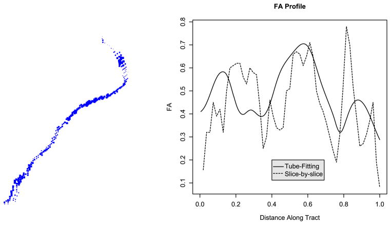
Figure 11 shows a single subject’s left cortico-spinal tract with image points scaled by FA value, and the FA profile generated using both the tube-fitting algorithm and the slice-by-slice approach. Note that the tube-fitting approach results in a smoother profile. More importantly, the tube-fitting method gives a profile that follows the course of the tract and accurately represents FA values at each position along the tract, whereas the slice-by-slice approach gives FA values in a given imaging plane.

Fig. 11.

On the left, we show the left cortico-spinal tract scaled by FA value. On the right, we show the FA profile constructed using the tube-fitting algorithm and using the slice-by-slice method.

7. Discussion

We have introduced a novel method for fitting three-dimensional tubes to imaging structures. Notably, we demonstrated the utility of the method on two very distinct imaging applications under different imaging modalities. In the colon SPECT imaging application, the tube-fitting method greatly improves upon previously used method of voxel-wise square neighborhoods. Moreover, our method produces an accurate mathematical model of the structure. Such characterization of the object of interest could be useful for subsequent shape analysis and for defining new measures of extent, volume and other features of anatomical structures.

With regard to future applications, we note that the ongoing SPECT study is now collecting dual-isotope images, with the goal of comparing the relative distribution of microbicidal lubricants and HIV-infected semen in the colon. Surrogates for both, tagged with tracers emitting gamma photons with different wavelengths, are injected at the same time and are simultaneously imaged. Such dual-isotope studies may lead to drastically improved fits—using image data from both tracers greatly increases the number of points available for our curve- and tube-fitting algorithms. However, these studies raise the problem of accurately distinguishing and characterizing two tracer distributions in the colon. Moreover, the study now collects images serially at several time points, giving us the opportunity to study changes in the concentration-by-distance curves over time. We are currently investigating the use of the accompanying X-ray computed tomography image for registration across time. Also, determining an anatomical landmark to compare curves across subjects remains difficult. We anticipate that bone landmarks from the CT image could be used to solve this problem, though we acknowledge that the colon can be fairly mobile across time and it’s relation to bones may not be straightforward.

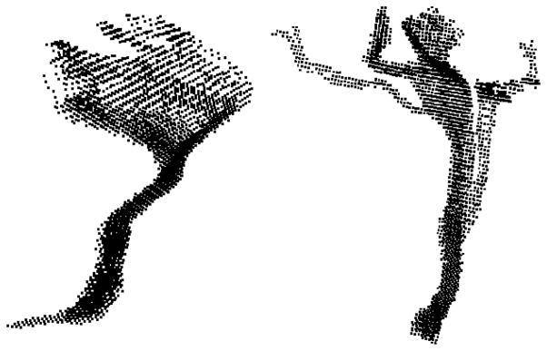
In the case of DTI tractography, the application of the tube-fitting algorithm to longitudinal images of multiple sclerosis patients will provide measures of disease progression. Ideally, one could use these measures to provide clinical evidence for the effectiveness of treatments. Validating the prediction performance of such measures remains an important problem. Moreover, the curve-fitting technique may not be applicable to all tracts (see Figure 12), and without an accurate centerline or without additional assumptions such as spatial contiguity of all points within the tract (so that the sampled tracts shown here can be considered nonrandom under-samplings), the tube-fitting algorithm will not work. A possible solution could be to adapt the curve-fitting technique found in Chung et al. (2010) that uses tractography path information for use in these more difficult tracts. Also, we are currently only using tracts created after ample preprocessing. Quantities derived from the original DTI image, such as anisotropy or diffusivity measurements, may produce more informative summaries of the tube. It is also possible that tube-fitting for this problem is best integrated into the tractography algorithm, which we have currently treated as a completely separate preprocessing step. Alternatively, the tensor itself could potentially be used to derive the individual tubes, obviating the need for tractography. However, we note that the fact that our algorithm only relies on existing tractography algorithms is also a strength, as it can be immediately applied.

Fig. 12.

Example corticospinal tracts for which the curve-fitting algorithm (and therefore the tube-fitting algorithm) fails.

We also note that one of the most important white matter tracts, the corpus callosum, which connects the left and right hemispheres of the brain, is not a tube-like structure. Instead it is more of a surface, with no clear centerline. Clearly, to analyze such structures a different approach is necessary. We are investigating the possibility of using principal surfaces for this task [Leblanc and Tibshirani (1994); Chang et al. (2001)].

A related problem germane to both application is the study of curves and tubes across individuals and across time. For example, the analysis of the volume/distance curves or the analysis of other features estimated by the tube remains an open question.

The curve-fitting algorithm itself could be improved. As seen above, it is not universally applicable. Moreover, a more automated algorithm with less user input is desirable. We are currently experimenting with a new stochastic search algorithm for finding centerlines, such as the use of genetic algorithms and simulated annealing. A benefit of these approaches is the wide range of objective functions which can be constructed to force a desired curve fit.

The tube-fitting algorithm presented here is a novel approach for the estimation of the the support of distributions in three dimensions. It is limited in that it requires the support to have a reasonable centerline and in that it uses ellipses to estimate the cross-sectional extent. However, it has proved a useful algorithm in two applications and holds a good deal of potential to be utilized in the field of medical imaging.

References

- Banfield JD, Raftery AE. Ice floe identification in satellite images using mathematical morphology and clustering about principal curves. J Amer Statist Assoc. 1992;87:7–16. [Google Scholar]
- Basser P, Mattiello J, LeBihan D. Estimation of the effective self-diffusion tensor from the NMR spin echo. J Magn Reson B. 1994a;103:247–254. doi: 10.1006/jmrb.1994.1037. [DOI] [PubMed] [Google Scholar]
- Basser P, Mattiello J, LeBihan D. MR diffusion tensor spectroscopy and imaging. Biophys J. 1994b;66:259–267. doi: 10.1016/S0006-3495(94)80775-1. [DOI] [PMC free article] [PubMed] [Google Scholar]
- Basser P, Pierpaoli C. Microstructural and physiological features of tissues elucidated by quantitative-diffusion-tensor MRI. J Magn Reson B. 1996;111:209–219. doi: 10.1006/jmrb.1996.0086. [DOI] [PubMed] [Google Scholar]
- Basser P, Pajevic S, Pierpaoli C, Duda J. In vivo fiber tractography using DT-MRI data. Magn Reson Med. 2000;44:625–632. doi: 10.1002/1522-2594(200010)44:4<625::aid-mrm17>3.0.co;2-o. [DOI] [PubMed] [Google Scholar]
- Beaulieu C. The basis of anisotropic water diffusion in the nervous system—a technical review. NMR Biomed. 2002;15:435–455. doi: 10.1002/nbm.782. [DOI] [PubMed] [Google Scholar]
- Bitter I, Sato M, Bender M, Kaufman A, Wan M, Wax M. Automatic, accurate and robust colon centerline algorithm. Radiology. 2000a;217(Suppl 705):370. [Google Scholar]
- Bitter I, Sato M, Bender M, McDonnell K, Kaufman A, Wan M. CEASAR: A smooth, accurate and robust centerline extraction algorithm. Proc. of IEEE Visualisation; Salt Lake City, UT. 2000b. pp. 45–52. [Google Scholar]
- Caffo BS, Crainiceanu CM, Deng L, Hendrix CW. A case study in pharmacologic colon imaging using principal curves in single photon emission computed tomography. J Amer Statist Assoc. 2009;103:1470–1480. doi: 10.1198/016214508000000832. [DOI] [PMC free article] [PubMed] [Google Scholar]
- Chang KY, Ghosh J, Inc I, Sunnyvale C. A unified model for probabilistic principal surfaces. IEEE Trans Pattern Anal Mach Intell. 2001;23:22–41. [Google Scholar]
- Chaudhuri P, Khandekar R, Sethi D, Kalra P. An efficient central path algorithm for virtual navigation. Proceedings of the Computer Graphics International (CGI’04); Washington, DC: IEEE Computer Society; 2004. pp. 188–195. [Google Scholar]
- Chiou R, Kaufman A, Liang Z, Hong L, Achniotou M. Interactive path planning for virtual endoscopy. Proceedings of the IEEE Nuclear Science and Medical Imaging Conference; Toronto, ON. 1998. pp. 2069–2072. [Google Scholar]
- Chiou R, Kaufman A, Liang Z, Hong L, Achniotou M. An interactive fly-path planning using potential fields and cell decomposition for virtual endoscopy. IEEE Trans Nuclear Sci. 1999;46:1045–1049. [Google Scholar]
- Chung MK, Adluru N, Lee J, Lazar M, Lainhart J. Cosine series representation of 3d curves and its application to white matter fiber bundles in diffusion tensor imaging. Statist Interface. 2010;3:69–80. doi: 10.4310/sii.2010.v3.n1.a6. [DOI] [PMC free article] [PubMed] [Google Scholar]
- Cohen L, Kimmel R. Global minimum for active contour models: A minimal path approach. J Comput Vision. 1997;24:57–78. [Google Scholar]
- Cohen E, Riesenfeld RF, Elber G. Geometric Modeling With Splines: An Introduction. A.K. Peters; Natick, MA: 2001. [Google Scholar]
- Deng L. Master’s thesis. Dept. Biostatistics, Johns Hopkins Univ; 2007. Spline-based curve fitting with applications to kinetic imaging. [Google Scholar]
- Deschamps T, Cohen L. Fast extraction of minimal paths in 3D images and applications to virtual endoscopy. Med Image Anal. 2001;5:281–299. doi: 10.1016/s1361-8415(01)00046-9. [DOI] [PubMed] [Google Scholar]
- Dijkstra E. A note on two problems in connexion with graphs. Numer Math. 1959:1 269–271. MR0107609. [Google Scholar]
- Hastie TJ. Principal curves and surfaces Technical Report 11. Laboratory for Computational Statistics, Dept. Statistics, Stanford Univ; 1984. [Google Scholar]
- Hastie TJ, Stuetzle WJ. Principal curves. J Amer Statist Assoc. 1989;84:502–516. MR1010339. [Google Scholar]
- Hastie TJ, Tibshirani R, Friedman J. The Elements of Statistical Learning. Springer; New York: 2001. MR1851606. [Google Scholar]
- Hendrix CW, Cao YJ, Fuchs EJ. Topical microbicides to prevent HIV: Clinical drug development challenges. Annu Rev Pharmacol Toxicol. 2009;49:349–375. doi: 10.1146/annurev.pharmtox.48.113006.094906. [DOI] [PubMed] [Google Scholar]
- Hendrix CW, Fuchs EJ, Macura KJ, Lee LA, Parsons TL, Bakshi RP, Khan WA, Guidos A, Leal JP, Wahl R. Quantitative imaging and sigmoidoscopy to assess distribution of rectal microbicide surrogates. Clin Pharmacol Ther. 2008;83:97–105. doi: 10.1038/sj.clpt.6100236. [DOI] [PubMed] [Google Scholar]
- Hong L, Muraki S, Kaufman A, Bartz D, He T. Virtual voyage: Interactive navigation in the human colon. Proceedings of SIGGRAPH; Los Angeles, CA.. 1997. pp. 27–34. [Google Scholar]
- Hudson H, Larkin R. Accelerated image reconstruction using ordered subsets of projection data. IEEE Trans Med Imaging. 1994;13:601–609. doi: 10.1109/42.363108. [DOI] [PubMed] [Google Scholar]
- Jiang H, van Zijl PC, Kim J, Pearlson GD, Mori S. DtiStudio: Resource program for diffusion tensor computation and fiber bundle tracking. Comput Methods Programs Biomed. 2006;81:106–116. doi: 10.1016/j.cmpb.2005.08.004. [DOI] [PubMed] [Google Scholar]
- Kegl B, Krzyzak A, Linder T, Zeger K. Learning and design of principal curves. IEEE Trans Pattern Anal Mach Intell. 2000;22:281–297. [Google Scholar]
- Kreyszig E. Differential Geometry. Dover Publications; New York: 1991. MR1118149. [Google Scholar]
- LeBihan D, Mangin J, Poupon C, Clark C. Diffusion tensor imaging: Concepts and applications. J Magn Reson Imaging. 2001;13:534–546. doi: 10.1002/jmri.1076. [DOI] [PubMed] [Google Scholar]
- Leblanc M, Tibshirani R. Adaptive principal surfaces. J Amer Statist Assoc. 1994;89:53–64. [Google Scholar]
- McFarland E, Wang G, Brink J, Balfe D, Heiken J, Vannier M. Spiral computed tomographic colonography: Determination of the central axis and digital unraveling of the colon. Acad Radiol. 1997;4:367–373. doi: 10.1016/s1076-6332(97)80119-5. [DOI] [PubMed] [Google Scholar]
- Mori S, Barker P. Diffusion magnetic resonance imaging: Its principle and applications. Anat Rec New Anat. 1999;257:102–109. doi: 10.1002/(SICI)1097-0185(19990615)257:3<102::AID-AR7>3.0.CO;2-6. [DOI] [PubMed] [Google Scholar]
- Mori S, Crain BJ, Chacko VP, van Zijl PC. Three-dimensional tracking of axonal projections in the brain by magnetic resonance imaging. Ann Neurol. 1999;45:265–269. doi: 10.1002/1531-8249(199902)45:2<265::aid-ana21>3.0.co;2-3. [DOI] [PubMed] [Google Scholar]
- Mori S, van Zijl PC. Fiber tracking: Principles and strategies—a technical review. Ann Neurol. 2002;15:468–480. doi: 10.1002/nbm.781. [DOI] [PubMed] [Google Scholar]
- Mori S, Wakana S, van Zijl PCM, Nagae-Poetscher LM. MRI Atlas of Human White Matter. Elsevier; Amsterdam: 2005. [Google Scholar]
- Reich DS, Smith SA, Jones CK, Zackowski KM, van Zijl PC, Calabresi PA, Mori S. Quantitative characterization of the corticospinal tract at 3T. Am J Neuroradiol. 2006;27:2168–2178. [PMC free article] [PubMed] [Google Scholar]
- Reich DS, Smith SA, Zackowski KM, Gordon-Lipkin EM, Jones CK, Farrell JA, Mori S, van Zijl PC, Calabresi PA. Multiparametric magnetic resonance imaging analysis of the corticospinal tract in multiple sclerosis. Neuroimage. 2007;38:271–279. doi: 10.1016/j.neuroimage.2007.07.049. [DOI] [PMC free article] [PubMed] [Google Scholar]
- Reich DS, Zackowski KM, Gordon-Lipkin EM, Smith SA, Chodkowski BA, Cutter GR, Calabresi PA. Corticospinal tract abnormalities are associated with weakness in multiple sclerosis. Am J Neuroradiol. 2008;29:333–339. doi: 10.3174/ajnr.A0788. [DOI] [PMC free article] [PubMed] [Google Scholar]
- Reich DS, Smith SA, Gordon-Lipkin EM, Ozturk A, Caffo BS, Balcer LJ, Calabresi PA. Damage to the optic radiation in multiple sclerosis is associated with retinal injury and visual disability. Arch Neurol. 2009;66:998–1006. doi: 10.1001/archneurol.2009.107. [DOI] [PMC free article] [PubMed] [Google Scholar]
- Samara Y, Fiebich M, Dachman A, Doi K, Hoffmann KR. Automated centerline tracking of the human colon. Proceedings of the SPIE Conference on Image Processing; Bellingham, WA: SPIE; 1998. pp. 740–746. [Google Scholar]
- Samara Y, Fiebich M, Dachman A, Kuniyoshi J, Doi K, Hoffmann KR. Automated calculation of the centering of the human colon on CT images. Acad Radiol. 1999;6:352–359. doi: 10.1016/s1076-6332(99)80230-x. [DOI] [PubMed] [Google Scholar]
- Thorpe JA. Elementary Topics in Differential Geometry. Springer; New York: 1979. MR0528129. [Google Scholar]
- Woods RP, Cherry SR, Mazziotta JC. Rapid automated algorithm for aligning and reslicing PET images. J Comput Assist Tomogr. 1992;16:620–633. doi: 10.1097/00004728-199207000-00024. [DOI] [PubMed] [Google Scholar]