Novel scatter compensation of list-mode PET data using spatial and energy dependent corrections

Abstract

With the widespread use of PET crystals with greatly improved energy resolution (e.g., 11.5% with LYSO as compared to 20% with BGO) and of list-mode acquisitions, the use of the energy of individual events in scatter correction schemes becomes feasible. We propose a novel scatter approach that incorporates the energy of individual photons in the scatter correction and reconstruction of list-mode PET data in addition to the spatial information presently used in clinical scanners. First, we rewrite the Poisson likelihood function of list-mode PET data including the energy distributions of primary and scatter coincidences and show that this expression yields an MLEM reconstruction algorithm containing both energy and spatial dependent corrections. To estimate the spatial distribution of scatter coincidences we use the single scatter simulation (SSS). Next, we derive two new formulae which allow estimation of the 2D (coincidences) energy probability density functions (E-PDF) of primary and scatter coincidences from the 1D (photons) E-PDFs associated with each photon. We also describe an accurate and robust object-specific method for estimating these 1D E-PDFs based on a decomposition of the total energy spectra detected across the scanner into primary and scattered components. Finally, we show that the energy information can be used to accurately normalize the scatter sinogram to the data. We compared the performance of this novel scatter correction incorporating both the position and energy of detected coincidences to that of the traditional approach modeling only the spatial distribution of scatter coincidences in 3D Monte Carlo simulations of a medium cylindrical phantom and a large, non uniform NCAT phantom. Incorporating the energy information in the scatter correction decreased bias in the activity distribution estimation by ~20% and ~40% in the cold regions of the large NCAT phantom at energy resolutions 11.5 and 20% at 511 keV, respectively, compared to when using the spatial information alone.

I. Introduction

Compton scattering of gamma photons in the patient affects quantification and reduces contrast, especially in 3D mode and in large patients where the scatter fraction (defined as the ratio of scatter coincidences divided by primary plus scatter coincidences) is frequently greater than 50%. Many scatter corrections exist that are based on the estimation of a scatter sinogram and its incorporation in the projector of an iterative reconstruction algorithm. Two of these approaches, the Monte Carlo simulation (MC) [1]–[3] and the single scatter simulation (SSS) [4], incorporate a detailed description of the Compton scattering process and are robust in the case of complex, non uniform attenuation and activity maps. However, MC and SSS depend on the unknown activity distribution and yield sinograms that require scaling to the data. These drawbacks can introduce important biases in the estimation of the activity distribution. Indeed, presence of scatter in the data affects the accuracy of the initial estimation of the activity map and therefore that of the scatter sinogram; while normalizing the scatter sinogram using the traditional “tail fitting” approach (which consists in fitting the tails of the scatter sinogram to the counts detected outside of the patient) can be very noisy and inaccurate when few coincidences are detected outside of the patient, e.g. in large patients and/or dynamic acquisitions [5].

In this work, we propose a new scatter correction that has the potential to mitigate these problems by modeling the energy distribution of primary and scattered coincidences in addition to their spatial distribution in the normalization and reconstruction processes. This strategy is motivated by the fact that the energy carries some probabilistic information about the status of detected photons, in increasing amount as the energy resolution of PET scanners improves. Moreover, the energy information is increasingly available in the list-mode files of modern PET scanners. Our approach is fundamentally different from existing techniques that use several large energy windows. Indeed, these energy window-based strategies use the energy indirectly in order to estimate a scatter sinogram [6]–[8], whereas we propose incorporating the individual energy of detected photons directly into the correction process, using a probabilistic model.

We describe the theoretical framework of our methodology in section II, which we then evaluate using realistic Monte Carlo simulations in sections III and IV.

II. Theory

A. Background

Very few authors, to our knowledge, have proposed using the individual energy of detected photons in the scatter correction of list-mode PET data. Levkovitz et al [9] and Chen et al [10] proposed similar approaches in which coincidences are weighted in the reconstruction procedure using an energy-dependent scheme. A major limitation of this approach is that these weights are not computed specifically for the object imaged but are either fixed to arbitrary values [9] or precomputed using Monte Carlo simulations of phantoms of different size and shapes [10]. Moreover, their inclusion in the reconstruction algorithm is not based on a rigorous statistical model of the data and might therefore yield biased estimates of the activity distribution. Popescu et al [11] proposed a more theoretically sound approach in which the energy probability density functions (E-PDFs) of scattered and primary coincidences are included in an MLEM reconstruction algorithm of list-mode PET data. They also proposed estimating the scatter sinogram using the energy information. As in the work of Chen et al and Levkovitz et al however, their energy model is based on energy basis functions that are pre-computed using Monte Carlo simulations of phantoms of different sizes and shapes.

Our approach is based on a reconstruction algorithm similar to that of Popescu et al incorporating both spatial and energy dependent corrections [11]. An important difference between our approach and those discussed above however is that it is based on an object-specific estimation of the primary and scattered coincidences E-PDFs. Another difference between our work and that of Popescu et al is that we do not attempt to use the energy information alone to scatter correct the data. Instead, we use it in addition to the scatter sinogram, computed independently with SSS, to improve the overall accuracy of the scatter correction.

In the rest of the paper, we note discrete probabilities Pr (.) and continuous densities P(.).

B. MLEM reconstruction algorithm of list-mode PET data with energy and spatial dependent corrections

1) List-mode log likelihood function with energy and scatter dependences

In the following we note ${\mathbf{E}}_n=\left(E_n^1,E_n^2\right)$ and ${\mathbf{X}}_n=\left(X_n^1,X_n^2\right)$ the vectors of energies and positions of the photons forming coincidence n, respectively. Using these notations, the Poisson log-likelihood function of list-mode data containing N coincidences, for which E_n and X_n are measured, is:

$$logL=\sum _{n=1}^{N}log\left({\alpha }_n{\sum }_{i=1}^M{a}_{ni}{\rho }_i{+}_n{S}_n\right)-\sum _{i=1}^M{s}_i{\rho }_i-\sum _{k=1}^K{S}_k-logN!,$$ (1)

where M is the number of image pixels, ρ is the unknown activity distribution, a_ni is the probability that a coincidence emitted from pixel i be detected in LOR X_n, s is the sensitivity image and S contains the average number of scatter coincidences detected in each of the K LORs of the scanner (i.e., the scatter sinogram). The terms α_n and β_n in Eq. (1) contain the dependence of the log-likelihood on the energy and are defined as α_n ≜ P (E_n | X_n, Pri.) and β_n ≜ P (E_n | X_n, Sca.), where “Pri.” and “Sca.” denote a primary and a scatter coincidence, respectively. In other words, α_n and β_n are 2D energy probability density functions (E-PDFs), depending a priori on the LOR X_n. Like the traditional log-likelihood function of list-mode PET data without scatter coincidences and energy terms, the log-likelihood of Eq. (1) is concave and therefore has a unique global maximum [12].

2) MLEM reconstruction of the activity distribution

Using a similar complete data space than the one used in [12], it is possible to show that an EM algorithm [13] maximizing the log-likelihood function in Eq. (1) is:

$${\rho }_j^{(a+1)}=\frac{{\rho }_j^{(a)}}{s_j}\sum _{n=1}^N\frac{{\alpha }_n{a}_{nj}}{{\alpha }_n{\sum }_{i=1}^M{\alpha }_{ni}{\rho }_i^{(a)}+{\beta }_n{S}_n},$$ (2)

where a is the iteration number. An outline of the derivation of this algorithm is shown in the Appendix. Eq. (2) is a reconstruction algorithm of list-mode PET data incorporating both spatial (via the scatter sinogram S) and energy dependent scatter corrections (via the E-PDFs α_n and β_n). It can account for random coincidences as well by adding them in the projector as follow: ${\alpha }_n{\sum }_{i=1}^M{a}_{ni}{\rho }_i^{(a)}+{\beta }_n{S}_n+R_n$. In the absence of randoms we note that Eq. (2) only depends on β/α, which is the likelihood ratio that one would form to test whether a coincidence is scattered or not, based on the energy of its photons. In other words, including the E-PDFs α and β in the reconstruction algorithm yields useful information when these distributions are the most different. In the extreme case where α = β, Eq. (2) in fact simplifies to the conventional MLEM reconstruction of list-mode data with only spatially dependent scatter corrections [14], [15].

C. Estimation of primary and scatter coincidence energy densities

In this section we present a new, object-specific method for computing the E-PDFs α and β.

1) Calculation of coincidences E-PDFs from photons E-PDFs

By definition, α ≜ P (E | X, Pri.) and β ≜ P(E | X, Sca.) are the 2D densities of primary and scatter coincidences’ vector of energies (Fig. 1). Estimating directly these 2D densities for every line of response is difficult in practice because very few coincidences are detected per LOR in a typical PET acquisition [16]. Instead, we propose decomposing α and β in terms of 1D photon E-PDFs that can be estimated with less noise.

Fig. 1.

A and B: Energy densities α and β obtained by histogramming the primary and scattered coincidences detected in a Monte Carlo simulation. C and D: Densities α and β estimated using Eqs. (3)–(6) and the primary and scatter photon spectra that were exactly known in this simulation. The densities C and D are very close to A and B but are less noisy since they were estimated from 1D photon’ spectra that contain fewer bins than 2D coincidences energy histograms.

As shown in Fig. 1(A), α is non negligible only when both photon energies are close to 511 keV as they must both be primary to form a primary coincidence. We have therefore:

$$\alpha =P(\mathbf{E}\mid \mathbf{X},\text{Pri}.)=P(E^1\mid \mathbf{X},\text{Pri}.)P(E^2\mid \mathbf{X},\text{Pri}.),$$ (3)

where E = (E¹, E²) is the vector of the photons’ energies and X = (X¹, X²) is the vector of the photons’ positions. A close form expression for β is more complex because there are three types of scattered coincidences: photon 1 is scattered and photon 2 is primary (type a); 1 is primary and 2 is scattered (type b) and both 1 and 2 are scattered (type c). The scattered coincidences of types a and b yield the edges of β along the axes E¹ = 511 keV and E² = 511 keV that are visible on Fig. 1(B), whereas those of type c account for the small plateau in the quadrangle of low energies. Applying Bayes rule to the definition of β yields:

$$\beta =P(\mathbf{E}\mid \mathbf{X},\text{Sca}.)=Pr(\text{Sca}.\mid \mathbf{E},\mathbf{X})P(\mathbf{E}\mid \mathbf{X})/Pr(\text{Sca}.\mid \mathbf{X}),$$ (4)

where the first factor in the numerator can be computed as:

$$Pr(\text{Sca}.\mid \mathbf{E},\mathbf{X})=\underset{\text{type}\text{a}}{\underbrace{Pr({\text{Sca}.}^1\mid E^1,\mathbf{X})Pr({\text{Pri}.}^2\mid E^2,\mathbf{X})}}+\underset{\text{type}\text{b}}{\underbrace{Pr({\text{Pri}.}^1\mid E^1,\mathbf{X})Pr({\text{Sca}.}^2\mid E^2,\mathbf{X})}}+\underset{\text{type}\text{c}}{\underbrace{Pr({\text{Sca}.}^1\mid E^1,\mathbf{X})Pr({\text{Sca}.}^2\mid E^2,\mathbf{X})}},$$ (5)

and the second factor as:

$$P(\mathbf{E}\mid \mathbf{X})=P(E^1\mid \mathbf{X})P(E^2\mid \mathbf{X}).$$ (6)

The normalization term P (Sca. | X) in Eq. (4) is simply obtained by summing the product Pr (Sca.| E, X)P (E | X) over all possible energies. We note that individual photon probabilities in Eqs. (3)–(6) depend on the line of response X and not only on their crystal of detection Xⁱ, since the spectra of photons detected in the same crystal but in different LORs are a priori different.

As shown in Fig. 2, the 1D photon densities in Eqs. (3)–(6) can be directly estimated from the knowledge of primary and scatter energy spectra in the crystals defining the LOR X.

Fig. 2.

Computation of the 1D probability Pr (Pri. | E) and the 1D density P (E | Pri.) using the local energy spectra of primary and scattered photons.

$$Pr(\text{Pri}.\mid E)=\frac{p}{p=s}P(E\mid \text{Pri}.)=\frac{p}{A}$$

2) Estimation of primary and scatter photons’ spectra

a) Binning of local energy spectra

As explained previously, estimating α and β using Eqs. (3)–(6) requires, in theory, knowing the primary and scattered photons’ spectra in every LOR of the scanner. This is not feasible in practice because a typical PET acquisition contains fewer coincidences (~ 100×10⁶) than the number of LORs in modern 3D PET scanners (~ 300 × 10⁶). Therefore, we propose estimating photon energy spectra in the crystals of the PET scanner rather than in its LORs. Even with this drastic reduction in the number of spectra to estimate (from ~ 300×10⁶ LORs to ~ 25,000 crystals), the number of spectra to be estimated is still considerable and, if needed, adjacent crystals can be grouped in large “sectors” in order to further reduce noise. Since the surface of the PET scanner roughly defines a cylinder, we propose decomposing it in polar sectors defined by their average angular position θ and their axial position z in the direction of the scanner’ axis. The total number of sectors in the axial (N_z) and angular (N_θ) directions must be chosen in order to minimize noise in the spectra, and therefore depends on the number of coincidences detected during the acquisition.

b)Decomposition of total spectra into primary and scatter components

Once the total energy spectra binned in N_z × N_θ polar sectors, these can be fitted with a model of local primary and scattered spectra. A simple fit is sufficient to estimate primary and scatter spectra because these distributions do not overlap at low energies, as shown in Fig. 2, except for primary photons that deposited a fraction of their energy in the detector that we therefore chose to treat as scattered photons. Doing so allows us to model primary spectra with Gaussian functions. For modeling scatter spectra, we propose using an object-specific factor model depending on a small number of scatter shapes. This model is based on the observation in Monte Carlo simulations that scatter spectra detected in the same axial sector z but in different angular sectors θ are, to a good approximation, proportional to the same shape (one factor can therefore be thought of as the average scatter spectra at a given axial position z). We propose estimating these scatter factors using a Monte Carlo simulation (MC), which is fast since estimating a few shapes requires simulating only a few tens of millions of coincidences. The activity and attenuation maps used as input of the MC simulation can be the same as those used in the SSS calculation (see section II. D. 1)). Combining the model of primary and scatter spectra described above yields the following model of the energy spectrum detected in the polar sector (z, θ):

$$A_{z,\theta }exp\left\{-\frac{{(E-511)}^2}{2{\sigma }_{z,\theta }^2}\right\}+B_{z,\theta }{F}_z(E),$$ (7)

where A_z,θ and B_z,θ are the amplitude of the primary and scatter components in sector (z, θ), σ_z,θ is the standard deviation of the primary spectrum in sector (z, θ) (i.e., the local energy resolution) and F_z (E) is the scatter factor at axial position z. When fitting Eq. (7) to total spectra, A_{z, θ} and σ_z,θ can be initialized to the height of the total spectrum at 511 keV and the average energy resolution of the scanner at 511 keV, respectively. B_z,θ can be initialized by imposing that the area under the total spectra at low energy, that we define here as E < 511 − 3σ_z,θ, is equal to the area under the scatter spectra.

D. Estimation of the scatter sinogram

1) Single scatter simulation

We propose estimating the scatter sinogram S using the single scatter simulation (SSS) that we implemented for the purpose of this study according to [4].

2) Normalization of the scatter sinogram

The scatter sinogram computed with SSS must be scaled to the data (a variant of SSS exists that is intrinsically normalized to the data but is systematically biased because of the absence of modeling of multiple scatter coincidences in SSS, and must therefore also be scaled in practice [15], [17], [18]). Since SSS only computes the scatter distribution in thick direct planes, the SSS sinogram is normalized to the data detected in the segment 0 (i.e., the segment containing the direct planes). The most common approach for normalizing the scatter sinogram to the data consists in fitting its tails to the coincidences detected outside of the boundaries of the object, which are usually estimated by thresholding the attenuation correction factors to a value close to 1 [15], [17], [18]. This method, called “tails fitting”, is not robust when few or no coincidences are detected outside the object, for example in large patients and in dynamic acquisitions (short frames). As an alternative to tails fitting, we propose a new normalization technique that computes scaling factors using both the position and energy information of all detected coincidences, not only those detected outside of the patient. An important advantage of this new normalization approach is that it does not depend on the scatter sinogram. In contrast with tails fitting, it is therefore accurate even in the presence of errors in the estimation of the shape of the scatter sinogram due, for example, to the absence of modeling of multiple scatter in SSS and errors in the initial estimation of the activity distribution (the accuracy of this global scaling step does not guarantee that the overall scatter correction is exact however. Even correctly scaled, a scatter sinogram with a wrong shape will eventually introduce a nonuniform bias in the estimation of the activity distribution).

By interpreting the scatter fraction (SF) as the marginal probability of a coincidence being scatter, integrated over all energies, we have:

$$\begin{array}{l}{SF}_k=Pr(\text{Sca}.\mid k)\\ =\int Pr(\text{Sca}.\mid \mathbf{E},k)P(\mathbf{E}\mid k)d\mathbf{E},\\ \approx \frac{1}{N}\sum _{n=1}^{N}Pr(\text{Sca}.\mid {\mathbf{E}}_n,k)\end{array}$$ (8)

where SF_k is the scatter fraction in the direct plane k (the last term in Eq. (8) is a Monte Carlo approximation of the marginal integral). Note that this sum is performed only over coincidences detected in the direct plane k of segment 0). The probability of one coincidence to be scattered can itself be computed using our previous decomposition of primary and scatter energy spectra according to:

$$Pr(\text{Sca}.\mid {\mathbf{E}}_n,k)=1-Pr\left(\text{Pri}.\mid E_n^1,{\mathbf{X}}_n\right)Pr\left(\text{Pri}.\mid E_n^2,{\mathbf{X}}_n\right).$$ (9)

Note that Eq. (9) must be evaluated using spectra containing only those photons detected in the segment 0 since the 2D energy distributions of coincidences detected in different segments are a priori different (in general, the energy probabilities for a group of coincidences must be computed using the spectra containing only the coincidences in that group). For a given acquisition, two series of spectra must therefore be estimated separately: one series containing all detected photons (series 1) and another containing only the photons involved in coincidences detected in segment 0 (series 2). Series 1 is used to compute energy probabilities in the reconstruction step whereas series 2 is used to compute energy probabilities in the normalization step.

As explained in section II. C. 2) a), Eq. (9) requires, in theory, knowing the primary and scatter spectra in all the LORs of the scanner, which is not feasible in practice. Using our decomposition of spectra detected in large polar sectors to compute Pr (Pri. | E, X) in Eq. (9) may introduce bias in the estimation of the SF. In particular, this approach never yields Pr (Sca. | E, k) = 1 even for coincidences detected outside of the object, because the spectra involved in this calculation are averaged over many LORs, some of them crossing the object and therefore containing primary photons. To reduce potential bias in the estimation of the SF due to this effect, we propose estimating Pr (Sca.| E, k) using Eqs. (8) and (9) when a coincidence is detected inside the object but imposing Pr (Sca. | E, k) = 1 when it is detected outside of the object (it is necessarily a scatter coincidence in that case).

E. Summary of the proposed approach

Fig. 3 shows the main steps of our energy and spatially dependent scatter correction as well as those of the conventional spatial scatter correction using SSS and tails fitting.

Fig. 3.

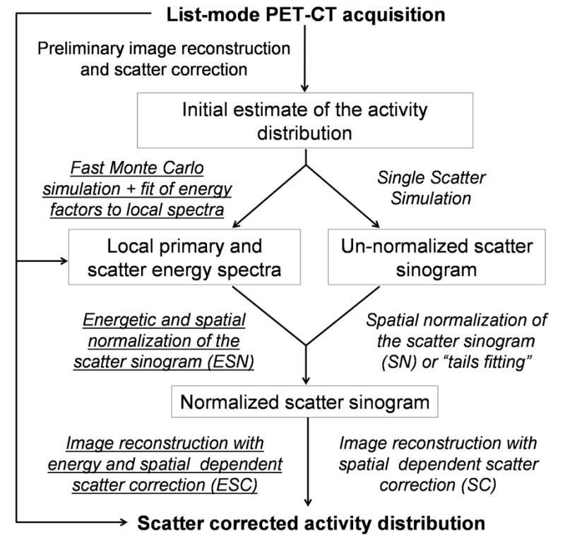
Flow chart summarizing the main steps of the proposed energy and spatially dependent scatter correction (italic underlined) and those of the conventional spatial correction strategy using SSS and tails fitting (italic).

We summarize here the main assumptions of our proposed approach:

1. Since it is not feasible in practice to compute the densities α and β for every line of response of the scanner according to Eqs. (3)–(6), we assume that the 1D energy densities involved in these equations depend only on the crystal of interaction of individual photons and not on the crystal of interaction of their coincidence partner.

2. To further reduce the number of spectra to estimate, we propose estimating the average energy spectra corresponding to groups of crystals rather than individual crystals. These groups of crystals are large polar sectors spanning the entire surface of the PET scanner.

3. To estimate energy spectra in these large polar sectors, we propose fitting them with a model in which primary spectra are modeled using Gaussian functions with varying amplitudes and widths.

4. In this model, scatter spectra in the same axial sector but in different angular sectors are assumed to be proportional to a small number of axial scatter shapes. These shapes are computed using a fast Monte Carlo simulation using initial estimates of the emission and attenuation maps.

5. Since our approach uses the energy information in addition to the scatter sinogram computed with SSS, it assumes, like SSS, that the spatial distribution of scatter coincidences in cross planes is the same as in direct planes [4].

III. Evaluation using Monte Carlo Simulations

We evaluated the performance of our scatter correction and compared it to that of the conventional spatial correction strategy using realistic Monte Carlo (MC) simulations of a medium and a large phantom.

A. Monte Carlo simulations

We modeled a medium cylindrical phantom (uniform attenuation) and a large anthropomorphic phantom (non uniform attenuation) using the NCAT phantom [19] shown in Fig. 4.

Fig. 4.

A: Medium sized (40 cm × 30 cm cross section and 20 cm axial extent) cylindrical phantom with hot (H) and cold (C) cylinders and uniform attenuation. Two hot cylinders of 20 cm diameter, 10 cm axial extent and activity 3/5^th of the background were also simulated at each end of the main phantom to model out-of-field activity. B: NCAT phantom of a large patient (51 cm × 40 cm cross section and 34 cm axial extent) with tumors and non uniform attenuation. The background activity is equal to 1 in both phantoms, by convention.

We modeled the block-based Philips Gemini TF PET/CT scanner using a realistic Monte Carlo simulation that we developed and validated previously [3]. This LYSO system is composed of 28 large detector panels containing 23 (transaxial)×44 (axial) crystals of size 4 × 4 × 22 mm³. The Gemini TF is a time-of-flight (TOF) PET scanner operating only in 3D mode, with excellent energy resolution (11.5% at 511 keV) and the capability of recording the energy of every detected photon in the output list file [20]. No variance reduction techniques were used in these list-mode simulations. Positron range and annihilation photons non-colinearity were modeled. Multiple scattering and partial interaction of gamma photons in the blocks of the Gemini TF were modeled as well as the loss of spatial resolution due to light sharing between the crystals of the same block. The energy, position, distance since annihilation and number of Compton scattering of every coincidence photon were recorded in the output list files.

We simulated 30.10⁹ (100.10⁹) coincidences in 533 (2167) hours distributed on 10 processors, resulting in the detection of 354.10⁶ (908.10⁶) valid coincidences for the medium (large NCAT) phantom. Ten list files containing each 90.10⁶ (340.10⁶) coincidences were then obtained by randomly sampling the coincidences of the main file with replacement, i.e. coincidences from the main list-file were chosen randomly and were possibly picked several times. This uniform bootstrap technique is widely used to generate multiple samples (here the small sub-files) from an observed distribution (here the main list file) and preserved the Poisson distribution of the data [21]–[23]. It allowed us to generate 10 list-mode noise realizations while keeping computation time reasonable (the simulation of 10 independent noise realizations of the large NCAT phantom would otherwise have taken a cumulated time of 8814 hours, or 338 days).

The energy resolution of the scanner was not modeled in the Monte Carlo simulation but as a post-processing step which allowed us to generate several energy resolutions without having to re-simulate the entire list-mode datasets. Note that this strategy made it impossible to model different crystal densities (for all energy resolutions the same crystal density was modeled corresponding to that of LYSO crystals). Random energies were generated according to the following energy-dependent Gaussian distribution:

$$\begin{array}{c}P(E_{det}\mid E_{\text{true}})\propto exp\left\{-\frac{{(E_{det}-E_{\text{true}})}^2}{2{\sigma }_i^2}\right\}\\ {\sigma }_i={\sigma }_i^{511}\sqrt{E_{\text{true}}/511},\end{array}$$ (10)

where E_true is the exact energy deposited by a simulated photon within its crystal of interaction i and ${\sigma }_i^{511}$ is the standard deviation of the photoelectric peak at 511 keV in that crystal. In order to take into account the random and systematic variations of the energy resolution in different crystals, ${\sigma }_i^{511}$ was not fixed to the average energy resolution of the scanner but was allowed to vary from crystal to crystal. To do so, tables of the energy resolution in the crystals of the PET scanner were generated using a Gaussian distribution with full width at half maximum (FWHM) equal to 1% (in units of relative FWHM energy resolution at 511 keV), which reflected typical experimental values reported in the literature [24]. This distribution was centered on the average energy resolution of the scanner for crystals located in the middle of a block and on average values 2% and 1% greater for crystals located in corners and edges of blocks, respectively [24].

B. Single scatter simulation

The attenuation map used in input of SSS was the actual attenuation distribution blurred at the spatial resolution of a low dose CT acquisition (Gaussian kernel, 4 mm FWHM). As explained in [4], the SSS was performed in two iterations. In the first iteration, an initial estimate of the activity distribution was reconstructed without scatter correction on a low resolution grid (128 × 128 × 22 pixels with 4×4×8 mm³ voxel resolution in the x, y and z directions) using list-mode OSEM with 2 iterations and 20 time-ordered subsets, which allowed computing a first SSS sinogram. This first SSS sinogram was then normalized to the data using tails fitting (spectra were not yet estimated at that stage so our new normalization approach could not be used) and was used to scatter correct the data in the second iteration, yielding a more accurate estimate of the activity distribution and the scatter sinogram. SSS was performed using scatter centers placed randomly in large voxels (2.5 × 2.5 × 2.5 mm³) covering the entire attenuation map and associated with a linear attenuation coefficient greater than 0.005 cm⁻¹ [18] (this value was chosen to effectively remove scatter centers located outside of the object since the lowest attenuation coefficient in the body is μ_lung ≈ 0.02 cm⁻¹). The SSS sinogram was first computed on a coarse grid (128 × 128 × 15) and was then interpolated to the full sinogram size (311 × 322 × 87 in the transaxial×angular×axial directions) while accounting for the arc effect.

C. Estimation of local primary and scatter spectra

For both phantoms, we divided the scanner into 600 large polar sectors (N_z = 20 and N_θ = 30), which yielded energy spectra with a reasonable noise level. Spectra contained 40 bins spanning the energy range [300 keV; 665 keV]. For each phantom, five scatter factors were computed using the Monte Carlo code SimSET [25] by propagating 30.10⁶ coincidences in the attenuation map (the same map used in SSS) using variance reduction techniques (non absorption and stratification). We used SimSET in this simulation step, rather than the more realistic simulation software that we used to generate the list-mode data, in order to mimic mismatches between simulated and measured data that are inevitable in practice. The emission map was the same as the one used in SSS, but corrected for scatter using the final SSS sinogram. A cylindrical uniform LYSO detector was modeled in this fast MC step that roughly approximated the geometry of the Gemini TF. The energy resolution of the scanner was modeled by blurring the factors using Eq. (10) at the average resolution of the scanner. Eq. (7) was then least square fitted to local total spectra.

D. Correction/reconstruction of the activity distribution

The activity distribution was corrected for scatter and reconstructed using three strategies depending on whether or not the energy was included in the normalization and the reconstruction steps: SN-SC (spatial normalization + spatial correction), ESN-SC (energy and spatial normalization + spatial correction) and ESN-ESC (energy and spatial normalization + energy and spatial correction). These three strategies used the same SSS sinogram and only differed in whether or not the energy was incorporated in the normalization and reconstruction processes. All reconstructions were performed using the ordered subsets (OS) version of Eq. (2), with (ESC) or without (SC) incorporating the densities α and β in the reconstruction (all reconstruction were fully 3D with 20 time-ordered subsets, 10 iterations and corrected for sensitivity and attenuation in the system matrix).

IV. Results

A. Medium uniform phantom

1) Single scatter simulation

Fig. 5 shows one slice of the scatter sinogram estimated in iterations 1 and 2 of SSS for the uniform water-filled phantom at 20% energy resolution (results were similar at 11.5% at 511 keV). Also shown are the reference SSS sinogram computed using the true activity map and the actual, noisy sinogram of scatter coincidences that is known in these Monte Carlo simulations (summed over all slices to reduce noise).

Fig. 5.

SSS estimation of the scatter sinogram in two iterations for the first Poisson realization of the medium uniform phantom at energy resolution 20% at 511 keV. The SSS sinograms obtained at iterations 1 and 2 are compared to the reference SSS sinogram obtained using the reference activity map in the SSS calculation. Also shown is the Monte Carlo sinogram of scatter coincidences, which is known exactly in this simulation (we show here the sum of all slices in order to render the scatter structure more visible). The block sensitivity pattern is clearly visible on these sinograms.

The reference SSS sinogram very closely approximated the mean of the true MC scatter sinogram, indicating that the absence of modeling of multiple scatter coincidences in SSS was not a serious limitation for this phantom. Instead, the main source of error in SSS was inaccuracies in the estimation of the activity map due to the presence of scatter in the data. Indeed, absence of scatter correction in the iteration 1 of SSS introduced an overestimation of pixel intensities at the center of the activity map, creating an overestimation of the scatter sinogram also more pronounced at the center of the FOV. Using this scatter sinogram in the iteration 2 of SSS over-corrected the data, which in turn yielded an underestimation of the activity map and of the final scatter sinogram (see Fig. 5).

Errors in the estimation of the final SSS sinogram (iteration 2), computed with respect to the reference SSS sinogram and averaged over all bins, were 4.3% and 4.7% at energy resolutions of 11.5% and 20% at 511 keV, respectively. The error was slightly greater at energy resolution 20% than 11.5% at 511 keV because the energy window was larger at 20% ([388 keV; 665 keV]) than at 11.5% ([440 keV; 665 keV]) and therefore contained more scatter coincidences.

2) Estimation of local primary and scatter spectra

Fig. 6 shows our estimation of primary and scatter spectra for the medium uniform phantom at 20% at 511 keV in two sectors for the first Poisson realization of the uniform water-filled phantom (results were similar at 11.5% at 511 keV). Table I shows corresponding estimation errors averaged over the 10 Poisson realizations, all sectors and within the energy window. Errors on primaries were smaller than on scatters for both series of spectra because primary energy spectra were very well modeled by a Gaussian function, whereas our factor model of scatter spectra is based on approximations that were slightly violated in practice. Errors were also smaller for series 1 than series 2, because the spectra of series 2 (segment 0 only) contained fewer photons than those of series 1 (all photons) and were therefore noisier.

Fig. 6.

Estimation of primary and scatter spectra for the first Poisson realization of the uniform water-filled phantom at 20% at 511 keV, in polar sectors (z =1, θ = 1) and (z =10, θ =1) and for series 1 and 2.

TABLE I.

Average primary and scatter spectra estimation errors for the medium uniform phantom

11.5% at 511 keV	Error on primaries	Error on scatters
Series 1	1.5%	3.9%
Series 2	2.3%	5.9%
20% at 511 keV
Series 1	1.9%	3.8%
Series 2	3.1%	5.9%

We also note that our estimation of spectra was slightly biased at low energy. This is due to primary photons (511 keV) that deposited only a fraction of their energy in the detector, which we chose to incorporate in our model of scatter spectra. As explained in section II. C. 2) b), this strategy allowed use of a simple Gaussian model for primary energy spectra, which considerably simplified the estimation process, while accounting for these events in order to ensure that the shapes of total spectra were correctly modeled (partially detected primary photons were modeled in scatter spectra by simply adding these events to the scatter shapes during the fast Monte Carlo simulation step).

Overall, our modeling of primary and scatter spectra was accurate within 6% for primary and scatter spectra and energy resolutions of 11.5% and 20% at 511 keV in both series for this phantom. This low error is due to the fact that total spectra were averaged over a large number of crystals in order to keep the noise level relatively low. This averaging process also made our decomposition procedure relatively insensitive to the locally varying energy resolution in different crystals.

3) Normalization of the scatter sinogram

The scatter normalization factors computed with both SN and ESN for this phantom were very close to the reference (we do not show them here for lack of space, see Fig. 10 for an example of normalization factors). Indeed, SN errors, averaged over all slices and 10 Poisson realizations, were 1.5% and 2.7% at energy resolutions 11.5% and 20% at 511 keV, respectively. Average errors for ESN were 0.8% and 2.1% for resolutions 11.5% and 20% at 511 keV, respectively. Applying our ESN strategy using the reference primary and scatter spectra yielded errors of 0.7% and 1.7% at resolutions 11.5% and 20% at 511 keV, respectively. This shows that most of the error in ESN was not caused by errors in the estimation of spectra but was a systematic bias due to the fact that spectra were estimated in large groups of crystals rather than in the LORs of the scanner as explained in section II. B. 2) a). ESN was slightly more accurate than SN because it does not depend on the scatter sinogram and was therefore insensitive to errors in its estimation.

Fig. 10.

A: Total number of scatter coincidences detected in the direct planes of the scanner, estimated using SN and ESN for the first Poisson realization of the NCAT phantom at 11.5% at 511 keV. B: Same at 20% at 511 keV.

4) Absolute quantification of the activity distribution

Fig. 7 shows images of the first Poisson realization of the uniform water-filled phantom scatter corrected and reconstructed at energy resolutions 11.5% and 20% at 511 keV using SN-SC (spatial normalization – spatial corrections), ESN-SC (energy and spatial normalization – spatial correction) and ESN-ESC (energy and spatial normalization – energy and spatial dependent corrections).

Fig. 7.

Images of the medium uniform phantom reconstructed at energy resolutions 11.5% and 20% at 511 keV with SN-SC, ESN-SC and ESN-ESC. These are compared to the image of primary coincidences which constitute the reference of scatter correction at the noise level simulated. Images are identically scaled.

Fig. 8 shows contrast recovery coefficients (CRC), biases and signal-to-noise ratio (SNR) in different regions of the phantom reconstructed with SN-SC, ESN-SC, ESN-ESC and using primary coincidences alone. CRCs were defined as:

$${\mathit{CRC}}_{\mathit{hot}}=100\times \frac{{\mu }_{\mathit{hot}}/{\mu }_{\mathit{bkg}}-1}{{\mu }_{\mathit{hot}}^{\mathit{ref}}/{\mu }_{\mathit{bkg}}^{\mathit{ref}}-1},$$ (11)

for hot regions and:

$${\mathit{CRC}}_{\mathit{cold}}=100\times (1-{\mu }_{\mathit{cold}}/{\mu }_{\mathit{bkg}}),$$ (12)

for cold regions, where μ_roi is the mean of pixel values located in the region of interest roi. Biases with respect to primaries were defined as:

$$b_{\mathit{hot}}=100\times ({\mu }_{\mathit{hot}}-{\mu }_{\mathit{hot}}^{\mathit{prim}})/{\mu }_{\mathit{hot}}^{\mathit{prim}},$$ (13)

in hot regions and:

$$b_{\mathit{cold}}=100\times ({\mu }_{\mathit{cold}}-{\mu }_{\mathit{cold}}^{\mathit{prim}})/{\mu }_{\mathit{bkg}}^{\mathit{prim}},$$ (14)

in cold regions. Finally, SNRs were computed as:

$$\mathit{SNR}=\frac{\left|{\mu }_{\mathit{roi}}-{\mu }_{\mathit{bkg}}\right|}{\sqrt{{\sigma }_{\mathit{roi}}^2+{\sigma }_{\mathit{bkg}}^2}},$$ (15)

where σ_roi is the mean of the standard deviation of pixels located in the region of interest roi, computed over different noise realizations.

Fig. 8.

Quantification of images corrected for scatter and reconstructed with SN-SC, ESN-SC, ESN-ESC and using primary coincidences alone (reference) at energy resolutions 11.5% and 20% at 511 keV for the medium water-filled phantom. A: Average contrast recovery coefficients (CRC) ± standard deviation computed over 10 Poisson realizations. B: Average biases ± standard deviation computed over 10 Poisson realizations. C: signal-to-noise ratio computed over 10 Poisson noise realizations. A star indicates a CRC or bias value significantly different than that associated with SN-SC (p < 10⁻³).

CRC and bias values in Fig. 8 show that the incorporation of the energy information in both the normalization and reconstruction processes made statistically significant but numerically modest improvement in the quantification of the cold regions of the uniform water-filled phantom (CRC values were sometimes slightly greater for SN-SC, ESN-SC and ESN-ESC than for primaries, indicating a slight overcorrection for scatter). Moreover, incorporating the energy information in the scatter correction did not significantly improve the quantification in hot regions since these are less affected than cold regions by scatter coincidences and, therefore, to errors in the correction of this effect. Finally, we note that SNR values associated with SN-SC, ESN-SC and ESN-ESC were very close to the reference, indicating that the scatter correction did not significantly increase noise in reconstructed images. This is mainly due to the fact that SSS is an analytical calculation and therefore low noise estimation of the scatter sinogram and that the scaling procedure was relatively low noise with both SN and ESN for this phantom.

B. Large non-uniform NCAT phantom

1) Single scatter simulation

Fig. 9 shows the estimation of the scatter sinogram with SSS for the large non-uniform NCAT phantom at 20% at 511 keV (results were similar at 11.5% at 511 keV). As in the uniform water-filled phantom, the reference SSS sinogram closely approximated the mean of the actual Monte Carlo scatter sinogram, indicating that ignoring the effect of multiple scatter coincidences in SSS was not a serious limitation even in this large phantom.

Fig. 9.

Estimation of the scatter sinogram in two iterations with SSS in the first Poisson realization of the large NCAT phantom at energy resolution 20% at 511 keV.

Final SSS sinogram estimation errors averaged over all bins, were 9.6% and 14.2% at energy resolutions 11.5% and 20% at 511 keV, respectively. Errors were greater for this large phantom than the smaller, uniform water-filled phantom because of the greater scatter fraction and the greater attenuation correction factors that amplified the effect of scatter in the initial estimate of the activity distribution.

2) Estimation of local primary and scatter spectra

Table II shows errors in the estimation of energy spectra for this large NCAT phantom, averaged over the 10 Poisson realizations, all sectors and within the energy window (these spectra were very similar to those obtained for the uniform water-filled phantom, we do not show them here for lack of space). As in the uniform water-filled phantom, estimation errors were greater for scatter than primary spectra and for series 2 than series 1. Our modeling of primary and scatter spectra was accurate within 5% for this non-uniform large phantom at energy resolutions 11.5% and 20% at 511 keV and for both series of spectra. As for the uniform water-filled phantom, the relatively good accuracy of our estimation approach is mainly due to the fact that spectra were averaged over a large number of crystals which reduced noise and made the estimation procedure relatively insensitive to local variations of the energy resolution from crystal to crystal.

TABLE II.

Average primary and scatter spectra estimation errors for the large NCAT Phantom

11.5% at 511 keV	Error on primaries	Error on scatters
Series 1	1.2%	3.0%
Series 2	1.7%	4.6%
20% at 511 keV
Series 1	1.6%	3.6%
Series 2	2.4%	4.7%

3) Normalization of the scatter sinogram

Fig. 10 shows the total number of scatter coincidences in the direct axial planes of the scanner estimated with SN and ESN and compared to the reference. SN errors, averaged over all planes and 10 Poisson realizations, were 3.6% and 7.3% for resolutions 11.5% and 20% at 511 keV, respectively. Average errors for ESN were 1.0% and 1.4% for resolutions 11.5% and 20% at 511 keV, respectively. Estimation errors with ESN applied using the actual primary and scatter spectra were 1.1% and 1.0% at 11.5% and 20% at 511 keV, respectively. As for the uniform water-filled phantom, this shows that most of the error with ESN was due to a systematic bias of the method because spectra are estimated in large groups of crystals rather than in individual LORs. Whereas the accuracy of SN was significantly worse for this phantom than for the uniform water-filled phantom because of greater errors in the estimation of the scatter sinogram, the accuracy of ESN remained constant. This is because ESN does not depend on the scatter sinogram and is therefore accurate even in the presence of important errors in its estimation.

4) Absolute quantification of the activity distribution

Fig. 11 shows images of the large NCAT phantom reconstructed and corrected for scatter using SN-SC, ESN-SC and ESN-ESC and compared to the reference. An improvement of image quality associated with the progressive incorporation of the energy information in the normalization procedure (ESN-SC compared to SN-SC) and in the reconstruction algorithm (ESN-ESC compared to ESN-SC) is clearly visible on these.

Fig. 11.

Images of the large NCAT phantom reconstructed at energy resolutions 11.5% and 20% at 511 keV with SN-SC, ESN-SC and ESN-ESC. These are compared to the image of primary coincidences which constitute the reference of scatter correction at the noise level simulated. Images are identically scaled.

Fig. 12 shows CRC, bias and SNR values in different hot and cold regions of images of this large NCAT phantom corrected and reconstructed with SN-SC, ESN-SC and ESN-ESC at energy resolutions 11.5% and 20% at 511 keV. As reported for the uniform water-filled phantom, using the energy information in the normalization and the reconstruction significantly reduced bias and improved contrast in cold areas. However, the impact of the energy was much greater in this large phantom than in the smaller uniform phantom because errors in the estimation of the scatter sinogram were more important and SN-SC was heavily biased. The impact of the energy was also greater at 20% than 11.5% at 511 keV because errors in the estimation of the scatter sinogram were greater in that case. We note that the SNR values associated with SN-SC, ESN-SC and ESN-ESC in both cold and hot regions were systematically lower than the SNR in the primary image and that this underestimation was in the same proportion as the underestimation of contrasts. This loss of SNR was therefore entirely due to a loss of contrast and not to an increase in noise, which shows that scatter correction using the SSS sinogram with or without using the energy information did not significantly increase noise in reconstructed images.

Fig. 12.

Quantification of images corrected for scatter and reconstructed with SN-SC, ESN-SC, ESN-ESC and using primary coincidences alone (reference) at energy resolutions of 11.5% and 20% at 511 keV for the large NCAT phantom. A: Average contrast recovery coefficients (CRC) ± standard deviation computed over 10 Poisson realizations. B: Average biases ± standard deviation computed over 10 Poisson realizations. C: signal-to-noise ratio computed over 10 Poisson noise realizations. A star indicates a CRC or bias value significantly different than that associated with SN-SC (p < 10⁻³).

5) Utilization of ESN instead of SN in SSS

Despite a clear improvement in the accuracy of the quantification when incorporating the energy in the scatter correction, a non-negligible residual bias persisted in cold regions of the large NCAT phantom corrected for scatter and reconstructed with ESN-ESC. This residual error was due to errors in the estimation of the scatter sinogram that were not completely compensated by using the energy information. To further improve the accuracy of the scatter correction, and since we have shown that ESN-ESC is more accurate than SN-SC, we now propose using ESN-ESC instead of SN-SC for estimating the activity distribution that is used in SSS. Like the standard SSS calculation, this variant is in two iterations. First, a scatter sinogram is computed using SSS and a reconstructed image uncorrected for scatter. Scatter shapes are also estimated in that step using same activity map and the Monte Carlo/spectra fitting approach described in section II. C. Next, the activity distribution is re-estimated using ESN-ESC which allows estimation of a second, more accurate, scatter sinogram with SSS. Note that in this variant, energy spectra are estimated using an initial estimate of the activity distribution uncorrected for scatter since the energy spectra fitting is performed before the two iterations SSS calculation. Table III shows the average errors associated with such an energy spectra estimation for the large NCAT phantom at both energy resolutions 11.5% and 20% at 511 keV. These errors are extremely close to those associated with our previous spectra decomposition (see section IV. B. 2)), showing that the presence of scatter in the data does not significantly affect the accuracy of our estimation of primary and scatter energy spectra in the polar sectors of the scanner.

TABLE III.

Average primary and scatter spectra estimation errors for the large NCAT phantom

11.5% at 511 keV	Error on primaries	Error on scatters
Series 1	1.2%	2.9%
Series 2	1.6%	4.2%
20% at 511 keV
Series 1	1.6%	3.5%
Series 2	2.4%	4.5%

Using ESN-ESC instead of SN-SC in the second iteration of the SSS procedure yielded scatter sinogram estimation errors of 4.5% and 5.3% at energy resolutions 11.5% and 20% at 511 keV, respectively. These were significantly lower than the errors associated with SSS using SN-SC (see section IV. B. 1)), which is due to the fact that ESN-ESC improved the accuracy of the initial estimation of the activity map and therefore also that of the SSS sinogram. Incorporating these sinograms in the final correction/reconstruction of the activity distribution with ESN-ESC yielded bias values lower than 13% in all regions of the large phantom at both energy resolutions, 11.5% and 20% at 511 keV. This is close to the ideal performance, especially compared to SN-SC that was associated with bias values of ~25% and ~60% in the cold regions of this large phantom at energy resolutions 11.5% and 20% at 511 keV, respectively.

V. Discussion

We have described a new methodology for incorporating the energy of individual photons in the scatter correction and reconstruction of list-mode PET data in addition to the scatter sinogram computed with SSS. Our approach rigorously incorporates primary and scatter coincidences 2D energy probability density functions (E-PDFs) both in the normalization of the scatter sinogram and the reconstruction procedure.

We have shown using Monte Carlo simulations that our proposed energy and spatial strategy (ESN-ESC) is significantly more accurate than the standard spatial correction (SN-SC or SSS-“tails fitting”), especially in cold regions and large patients. Specifically, we found that using the energy in addition to the position information in the normalization and reconstruction steps reduced reconstruction biases and improved contrasts in cold regions of the large NCAT phantom by ~20% and ~40% at energy resolutions 11.5% and 20% at 511 keV, respectively. Improvements in SNR in the hot and cold regions of this large phantom closely followed the improvements in biases and contrasts, indicating that the correction process did not significantly increase noise in the final corrected image. As explained in section IV. B. 5), a nonnegligible residual bias was still present even in images reconstructed with ESN-ESC because of large errors in the estimation of the scatter sinogram that were not completely compensated by using the energy information. To further improve quantification, we propose a correction strategy that uses ESN-ESC both for estimating the initial activity map used by SSS and for reconstructing the final corrected image. Doing so reduced absolute quantification errors below 13% in all regions of the large NCAT phantom and at both energy resolution 11.5% and 20% at 511 keV.

Our results indicate that the traditional spatial correction SN-SC is accurate for medium sized patients at both energy resolution 11.5% and 20% at 511 keV. In large patients however, the initial estimation of the activity map was significantly biased due to the greater scatter fraction and the large attenuation correction coefficients (ACF) that considerably amplified the presence of scatter at the center of the FOV. Since the SSS calculation is linear in the activity distribution, this error propagated in the estimation of the scatter sinogram and caused a final underestimation of the scatter sinogram (this error was an overestimation in the first iteration of SSS and an underestimation in the second and final iteration). Incorporating the energy information in the normalization and reconstruction procedures partially compensated for this error.

We also found that neglecting the effect of multiple scattered coincidences in SSS was not a serious source of error, even in the large NCAT phantom at energy resolution 20% at 511 keV, since using the perfect activity map in SSS yielded an almost ideal estimation of the scatter sinogram. This result is not in contradiction to a previous study by Adams et al [26] in which the authors reported very different spatial profiles of single scattered (SS) coincidences and multiple scattered (MS) coincidences. Indeed, such profiles were obtained by simulating a point source in water whereas we simulated distributed objects. For a point source, SS profiles, unlike MS profiles, have sharp edges due to the energy cutoff and the relation between the Compton scattering angle and the scattered energy. Since distributed objects can be seen as the superposition of an infinite number of point sources, sharp edges in the SS profiles of the individual point sources making up the object overlap to yield a smooth overall SS profile. Once the point source SS and MS distributions are convolved with the activity distribution imaged, the SS and MS distributions simulated by Adam et al [26] become in fact very similar.

The approach proposed in this work differs from scatter modeling techniques that simulate scatter in the system matrix in an attempt to use the fact that low angle scattered coincidences carry some information on the location of the radiotracer. Instead, our technique attempts to improve the rejection of scatter coincidences by using not only a spatial criterion but also an energetic one.

In this study, we evaluated our approach using detailed Monte Carlo simulations of the propagation of gamma photons in the patient and a realistic model of the PET detector. The main advantage of such simulations is that they provide perfect knowledge of the ground truth, i.e. the activity distribution and primary and scatter coincidences. This allowed us to objectively assess the overall accuracy of ESN-ESC and that of its individual modeling components (scatter sinogram estimation, normalization and energy spectra estimation). In an effort to make the simulation as realistic as possible, we modeled multiple interaction of gamma photons in the detector and used a Gaussian energy model that took into account the square root dependence of the energy resolution with the deposited energy as well as the random and systematic variation of the energy resolution in the crystals of real PET scanners [24]. Despite these efforts our simulation was necessarily a simplified model of real scanners, in particular because it did not model random coincidences and the imperfections of the electronic system. The study of these effects and their impact on the accuracy of ESN-ESC in practice is beyond the scope of this paper and will be the focus of a separate study; however a few general comments can be made about them. First, as noted in section II. B. 2), the spatial distribution of random coincidences can be modeled as usual in the projector of the reconstruction algorithm Eq. (2). Similarly, the contribution of random coincidences to total spectra can be modeled in our energy spectra estimation procedure by simply adding it to the primary and scatter components in Eq. (10) (note that the spatial and energetic distributions of random coincidences can be measured in real systems using a delayed coincidence window).

The problem of imperfect energy capture by the electronic system is more serious because this effect is difficult to model in our estimation of local primary and scatter spectra. In practice however, some degree of immunity of our method is provided by the fact that it does not attempt estimation of energy spectra in individual crystals but in large polar sectors containing many crystals (there were ~50 crystals per sectors in this study). This averaging process is crucial to reduce noise and to make our energy spectra estimation less sensitive to random fluctuations in the event-by-event performance of the electronic system responsible of measuring the energy. Note that systematic variations of the performance of the energy capture electronic system should be accounted for in the energy calibration procedure (in essence, we have assumed in this study that the energy calibration of the simulated system was perfect). Since accurate energy calibration is crucial to ensure good performance of the proposed approach, it might prove necessary in practice to calibrate the PET scanner energy capture electronics more often that what is done today.

A necessary next step in the evaluation of the approach proposed in this manuscript will involve its application to physical acquisition of phantom and human data. However, such an evaluation is beyond the scope of this work because it requires resolving important experimental difficulties (the practical application of the proposed approach will be the focus of separate study). Indeed, most PET scanners with the ability of measuring the energy in list-mode, including the Philips Gemini TF, yield accurate energy estimates only within the main energy window (e.g., between 440 keV and 665 keV for the Philips Gemini TF). This is because event triggering in the electronics is generally performed using a constant fraction discriminator that applies a rough low energy cut before energy estimation in order to reduce electronics dead-time. Since this trigger is performed in the electronics hardware before PMT gain calibrations, its lower energy edge is not defined accurately. In a real system, the value of this rough low energy cut is therefore chosen low enough to ensure that variations in the resulting effective energy threshold are not greater than the lower level discriminator of the main energy window, which is applied in software after PMT gain calibrations. This strategy guarantees that no “acceptable” photons are rejected and allows accurate estimation of the energy within the main energy window. Outside this main window however, it yields heavily biased energy estimates. Such difficulty in estimating the low energy tails of energy spectra makes it difficult at present to use the energy information in the scatter correction because, as explained in section II. C. 2) b), primary and scatter spectra are the most easily separable at low energies. To solve this problem, we will explore hardware solutions allowing better quantification of low energies. We will also explore methods for decomposing energy spectra into their primary and scatter components using only those photons detected in the main energy window.

We have chosen to evaluate the proposed approach and the standard spatial correction by reporting biases, contrasts and signal-to-noise ratio in reconstructed images. These figures of merit allowed us to objectively assess the improvement in image quality and quantification associated with incorporating the energy information in the scatter correction process. It may also be useful to assess the performance of our approach for specific clinical tasks like the detection of tumors and the quantification of myocardial perfusion.

VI. Conclusion

We have shown that using the energy information in addition to the scatter sinogram computed with SSS in the scatter correction procedure significantly improves the quantitative accuracy of reconstructed PET images, especially in cold regions and large patients. The most accurate scatter correction evaluated in this study included the energy and spatial information in the normalization (ESN) and reconstruction procedures (ESC), both in the SSS calculation and the final estimation of the activity distribution. Doing so yielded absolute quantification errors lower than 13% in all regions of the largest patient at energy resolutions 11.5% and 20% at 511 keV. This represented a substantial reduction of bias (~20% at 11.5% energy resolution and ~50% at 20% energy resolution) compared to the traditional approach using only the spatial information (SN-SC or SSS–tails fitting).

Appendix

In this section, we provide the main steps of the derivation of the MLEM algorithm in Eq. (2). Such a derivation requires writing the complete list-mode log-likelihood function as a function of the hidden parameters. To do so, we chose to parameterize the complete data-space in a manner similar to [12] using the vectors z_n, defined as z_ni = 1 if and only if coincidence n was emitted from voxel i (z_ni = 0 otherwise); and the scalars γ_n, defined as γ_n = 1 if and only if coincidence n is primary (γ_n = 0 otherwise). Using this parameterization, the complete log-likelihood function for N independent coincidences can be written as:

$$\begin{array}{l}logL=\sum _{n=1}^{N}logP({\mathbf{E}}_n,{\mathbf{X}}_n,{\mathbf{z}}_n,{\gamma }_n\mid \mathbf{\rho })+logPr(N\mid \mathbf{\rho })\\ =\sum _{n=1}^N\left\{{\gamma }_n\sum _{i=1}^M{z}_{ni}log[{\alpha }_n{a}_{ni}{\rho }_i]+(1-{\gamma }_n)log[{\beta }_n{S}_n]\right\}-\sum _{i=1}^M{s}_i{\rho }_i-\sum _{k=1}^K{S}_k-logN!,\end{array}$$ (16)

which holds because most z_ni and γ_n are zeros.

Applying the expectation step of the EM algorithm to Eq. (16) requires computing E [γ_nz_ni] and E [1 − γ_n]. Using Bayes rule, it is possible to show that:

$$\begin{array}{l}E[{\gamma }_n{z}_{ni}]=Pr(i,\text{Pri}.\mid {\mathbf{E}}_n,{\mathbf{X}}_n)\\ =\frac{1}{P({\mathbf{E}}_n,{\mathbf{X}}_n)}\frac{{\alpha }_n{a}_{ni}{\rho }_i^{(a)}{s}_i}{{\sum }_{j=1}^M{s}_j{\rho }_j^{(a)}+{\sum }_{k=1}^K{S}_k}\\ =\frac{{\alpha }_n{a}_{ni}{\rho }_i^{(a)}{s}_i}{{\alpha }_n{\sum }_{j=1}^M{a}_{nj}{\rho }_j^{(a)}{s}_j+{\beta }_n{S}_n},\end{array}$$ (17)

where P (E_n, X_n) is the Bayes’ normalization constant computed by summing the second ratio of the second line of Eq. (17) over all energies and primary and scattered coincidences. Similarly:

$$\begin{array}{l}E[1-{\gamma }_n]=Pr(\text{Sca}.\mid {\mathbf{X}}_n,{\mathbf{E}}_n)\\ =\frac{1}{P({\mathbf{E}}_n,{\mathbf{X}}_n)}\frac{{\beta }_n{S}_n}{{\sum }_{j=1}^M{s}_j{\rho }_j^{(a)}+{\sum }_{k=1}^K{S}_k}\\ =\frac{{\beta }_n{S}_n}{{\alpha }_n{\sum }_{j=1}^M{a}_{nj}{\rho }_j^{(a)}{s}_j+{\beta }_n{S}_n}.\end{array}$$ (18)

Finally, applying the M step of the EM algorithm consists in finding the new pixel intensities ρ^(a+1) maximizing the averaged complete log-likelihood. Differentiating this function twice shows that its global maximum is reached for:

$${\rho }_j^{(a+1)}=\frac{1}{s_j}\sum _{n=1}^{N}E\left[{\gamma }_n{z}_{nj}\right]=\frac{{\rho }_j^{(a)}}{s_j}\sum _{n=1}^N\frac{{\alpha }_n{a}_{nj}}{{\alpha }_n{\sum }_{i=1}^M{a}_{ni}{\rho }_i^{(a)}+{\beta }_n{S}_n}.$$ (19)

References

- 1.Holdsworth CH, Levin CS, Janecek M, Dalhbom M, Hoffman EJ. Performance analysis of an improved 3-D PET Monte Carlo simulation and scatter correction. IEEE Trans Nucl Sci. 2002;49:83–89. [Google Scholar]
- 2.Holdsworth CH, Levin CS, Farquhar TH, Dalhbom M, Hoffman EJ. Investigation of accelerated Monte Carlo techniques for PET simulation and 3D PET scatter correction. IEEE Trans Nucl Sci. 2001;48:74–81. [Google Scholar]
- 3.Guérin B, El Fakhri G. Realistic PET Monte Carlo Simulation with Pixellated Block Detectors, Light Sharing, Random Coincidences and Dead-time Modeling. IEEE Trans Nucl Sci. 2008;55:942–952. doi: 10.1109/TNS.2008.924064. [DOI] [PMC free article] [PubMed] [Google Scholar]
- 4.Watson CC. New, faster, image-based scatter correction for 3D PET. IEEE Trans Nucl Sci. 2000;47:1587–1594. [Google Scholar]
- 5.Zaidi H, Koral KF. Scatter modelling and compensation in emission tomography. Eur J Nucl Med Mol Imaging. 2004;31:761–782. doi: 10.1007/s00259-004-1495-z. [DOI] [PubMed] [Google Scholar]
- 6.Groontoonk S, Spinks TJ, Sashin D, Spyrou NM, Jones T. Correction for scatter in 3D PET using a dual energy window method. Phys Med Biol. 1996;41:2757–2774. doi: 10.1088/0031-9155/41/12/013. [DOI] [PubMed] [Google Scholar]
- 7.Ferreira NC, Trébossen R, Lartizien C, Brulon V, Merceron P, Bendriem B. A hybrid scatter correction for 3D PET based on an estimation of the distribution of unscattered coincidences: implementation on the ECAT EXACT HR+ Phys Med Biol. 2002;47:1555–1571. doi: 10.1088/0031-9155/47/9/310. [DOI] [PubMed] [Google Scholar]
- 8.Shao L, Freifelder R, Karp JS. Triple energy window scatter correction in PET. IEEE Trans Med Imag. 1994;13:641–648. doi: 10.1109/42.363104. [DOI] [PubMed] [Google Scholar]
- 9.Levkovitz R, Falikman D, Zibulevsky M, Ben-Tal A, Nemirovski A. The design and implementation of COSEM, an iterative algorithm for fully 3-D listmode data. IEEE Trans Med Imag. 2001;20:633–42. doi: 10.1109/42.932747. [DOI] [PubMed] [Google Scholar]
- 10.Chen HT, Kao CM, Chen CT. A fast, energy-dependent scatter reduction method for 3D-PET imaging. IEEE Nucl Sci Symp Med Imag Conf. 2003;4:2630–2634. [Google Scholar]
- 11.Popescu LM, Lewitt RM, Matej S, Karp JS. PET energy-based scatter estimation and image reconstruction with energy-dependent corrections. Phys Med Biol. 2006;51:2919–2937. doi: 10.1088/0031-9155/51/11/016. [DOI] [PubMed] [Google Scholar]
- 12.Parra L, Barrett H. List-Mode Likelihood: EM Algorithm and Image Quality Estimation Demonstrated on 2-D PET. IEEE Trans Med Imag. 1998;17:228–235. doi: 10.1109/42.700734. [DOI] [PMC free article] [PubMed] [Google Scholar]
- 13.Dempster P, Laird NM, Rubin DB. Maximum Likelihood from Incomplete Data via the EM Algorithm. J Roy Stat Soc B. 1977;39:1–38. [Google Scholar]
- 14.Qi J, Huesman RH. Scatter correction for positron emission mammography. Phys Med Biol. 2002;47:2759–71. doi: 10.1088/0031-9155/47/15/315. [DOI] [PubMed] [Google Scholar]
- 15.Werling A, Bublitz O, Doll J, Adam L-E, Brix G. Fast implementation of the single scatter simulation algorithm and its use in iterative image reconstruction of PET data. Phys Med Biol. 2002;47:2947–60. doi: 10.1088/0031-9155/47/16/310. [DOI] [PubMed] [Google Scholar]
- 16.Bentourkia M, Msaki P, Cadorette J, Lecomte R. Energy dependence of scatter components in multispectral PET imaging. IEEE Trans Med Imag. 1995;14:138–45. doi: 10.1109/42.370410. [DOI] [PubMed] [Google Scholar]
- 17.Watson CC, Casey ME, Michel C, Bendriem B. Advances in scatter correction for 3D PET/CT. Nul Sci Symp Med Imag Conf. 2004;5:3008 –3012. [Google Scholar]
- 18.Accorsi R, Adam L-E, Werner ME, Karp JS. Optimization of a fully 3D single scatter simulation algorithm for 3D PET. Phys Med Biol. 2004;49:2577–98. doi: 10.1088/0031-9155/49/12/008. [DOI] [PubMed] [Google Scholar]
- 19.Segars WP, Lalush DS, Tsui BMW. A realistic spline-based dynamic heart phantom. IEEE Trans Nucl Sci. 1999;46:503–506. [Google Scholar]
- 20.Surti S, Kuhn A, Werner ME, Perkins AE, Kolthammer J, Karp JS. Performance of Philips Gemini TF PET/CT Scanner with Special Consideration for Its Time-of-Flight Imaging Capabilities. J Nucl Med. 2007;48:471–480. [PubMed] [Google Scholar]
- 21.Ross SM. Introduction to probability models. Academic Press; 2001. [Google Scholar]
- 22.Haynor DH, Woods SD. Resampling estimates of precision in emission tomography. IEEE Trans Med Imag. 1989;8:337–343. doi: 10.1109/42.41486. [DOI] [PubMed] [Google Scholar]
- 23.Lartizien C, Aubin JB, Buvat I. Comparison of bootstrap resampling methods for 3-D PET imaging. IEEE Trans Med Imag. 2010;29:1442–1454. doi: 10.1109/TMI.2010.2048119. [DOI] [PubMed] [Google Scholar]
- 24.Williams JJ, McDaniel DL, Kim CL, West LJ. Detector characterization of Discovery ST whole-body PET scanner. Nul Sci Symp Med Imag Conf. 2003;2:717–721. [Google Scholar]
- 25.Harrison RL, Haynor DR, Gillispie SB, Vannoy SD, Kaplan MS, Lewellen TK. A public-domain simulation system for emission tomography: photon tracking through heterogeneous attenuation using importance sampling. J Nucl Med. 1993;34:60P. [Google Scholar]
- 26.Adam LE, Karp JS, Brix G. Investigation of scattered radiation in 3D whole-body positron emission tomography using Monte Carlo simulations. Phys Med Biol. 1999;44:2879–2895. doi: 10.1088/0031-9155/44/12/302. [DOI] [PubMed] [Google Scholar]