Abstract
The partially separable function (PSF) model has been successfully used to reconstruct cardiac MR images with high spatiotemporal resolution from sparsely sampled (k,t)-space data. However, the underlying model fitting problem is often ill-conditioned due to temporal undersampling, and image artifacts can result if reconstruction is based solely on the data consistency constraints. This paper proposes a new method to regularize the inverse problem using sparsity constraints. The method enables both partial separability (or low-rankness) and sparsity constraints to be used simultaneously for high-quality image reconstruction from undersampled (k,t)-space data. The proposed method is described and reconstruction results with cardiac imaging data are presented to illustrate its performance.
I. INTRODUCTION
Several model-based methods have been proposed to enable reconstruction from highly undersampled (k, t)-space data [1]–[5]. The partially separable function (PSF) model assumes that the (k, t)-space MR signal s(k, t) is partially separable to the Lth order [4] such that
| (1) |
where and can be treated as spatial and temporal basis functions, respectively. Due to strong spatiotemporal correlations in cardiac MR signals, L can usually be chosen to be very small [6], which significantly reduces the number of degrees of freedom of the model.
Consider the following Casorati matrix formed from the samples of s(k, t),
| (2) |
where N represents the number of k-space points at each time instant for a total of M instants in an ‘ideal’ data set . If s(k, t) is Lth-order partially separable, it is easy to show that the rank of S is upper bounded by L [4] and S can be decomposed as
| (3) |
where Vt ∈ ℂL×M is a basis for the temporal subspace of S, and Uk ∈ ℂN×L is a matrix of k-space coefficients. With sparse sampling, many entries of S are missing. The actual measured data can be expressed as
| (4) |
where d ∈ ℂp is the measured data, Ω: ℂN×M → ℂp is the sparse sampling operator, and ξ ∈ ℂp represents measurement noise. In this paper, we assume that Vt is known (i.e., predetermined from navigator signals as is done in [4], [6]) and our goal is to determine Uk from d. The basic PSF method solves the following unconstrained problem:
| (5) |
A necessary condition for (5) to be well-posed is that each k-space location is sampled at least L times. In practice, we need much more measurements to avoid a poorly conditioned inverse problem. In the previous work, spatial-spectral support information has been exploited to improve the conditioning of the problem and reduce reconstruction artifacts [7], [8].
In this paper, we use an (x, f)-domain sparsity constraint to regularize the inverse problem. An (x, f)-domain sparsity constraint has been used in previous work [9]–[11]. Our method is the first attempt to use both explicit partial separability and (x, f )-domain sparsity for image reconstruction from highly undersampled (k, t)-space data. The rest of paper is organized as follows: Section II describes the proposed formulation and image reconstruction algorithm; Section III presents an application of the proposed method to real-time cardiac MRI and discussion of related work, followed by a brief conclusion in Section IV.
II. PSF solution with sparsity constraint
Incorporating an (x, f)-domain sparsity constraint, the PSF reconstruction problem can be formulated as
| (6) |
where ℱs represents a spatial Fourier transform operator, Ft is a temporal Fourier transform matrix,
 , and λ is a regularization parameter. In the above expression, both ℱs and Ft are assumed to be orthonormal, and ||·||1 of a matrix is defined as the sum of the magnitudes of all entries in the matrix. The ℓ1 penalty (or ℓ1 regularization) in (6) has been widely used for finding sparse solutions to ill-posed inverse problems [12].
We propose to solve (6) using an additive half-quadratic regularization algorithm [11], [13], [14] and a continuation procedure [11], [15], [16]. First, the non-differentiable ℓ1 norm is replaced by a differentiable approximation
| (7) |
where ϕ(t): ℝ → ℝ is the Huber function defined as
| (8) |
Note that ϕ(t) is a continuously differentiable function, and the accuracy of the approximation in (7) is controlled by the parameter α. As α → 0, the Huber function approaches |t|. Furthermore, it can be shown that . Therefore, (7) can be rewritten as
| (9) |
where G is an auxiliary matrix and ||·||F denotes the Frobenius norm. Using (7) and (9), the problem in (6) can be approximated as
 |
(10) |
We solve (10) using an alternating optimization procedure, which first optimizes Us with a fixed value of G, and then optimizes G with a fixed value of Us. This procedure is repeated until Us and G converge. At the ℓth iteration and for a fixed , minimizing (10) over G is accomplished using the following soft-shresholding operation
| (11) |
where . With a fixed G(ℓ), minimizing (10) with respect to Us is equivalent to
 |
(12) |
By changing variables Uk = ℱsUs and B(ℓ) = FsG(ℓ)Ft, we can convert (12) into
| (13) |
Though (13) is a large-scale quadratic optimization problem, it has a simple decoupled structure, which enables very efficient evaluation. Specifically,
| (14) |
where represents the nth row of Uk, and Ωn is the sampling operator that takes samples from the nth row of UkVt. Thus, (13) is equivalent to solving
| (15) |
for 1≤n≤N, where dn is the measured data from the nth row of S, and is the nth row of B(ℓ). In (15), each quadratic optimization problem is equivalent to
 |
(16) |
for 1 ≤ n ≤ N, where
 (·) = Ωn(·Vt), ℬn(·) = ·Vt,
 and
and
 are the adjoint operators of
 and ℬn, respectively. Since each normal equations in (16) only has L unknowns, it can be solved very efficiently. For example, ideally the conjugate gradient method can solve (15) or (16) in only L iterations if the exact arithmetic is assumed [17]. Moreover, the completely decoupled structure is quite suitable for parallel computation for further computational accelerations.
The above alternating optimization procedure gives an optimal solution to (10). To obtain a good approximate to (6), a continuation scheme is used. The continuation procedure starts with a large value of α, which causes the alternating algorithm to converge rapidly [14]. Then we decrease the value of α in (10) and use the previous solution as a ‘warm start’ for the new alternating optimization. The above procedure is repeated until the cost function of (10) well approximates the cost function in (6).
III. Results and Discussion
A. Simulation Results
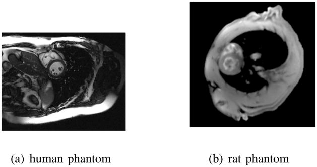
The proposed method has been validated systematically using both human and rat cardiac phantoms. These phantoms were used to simulate free-breathing cardiac imaging experiments with variable heartbeat periods. Snapshot images from two phantoms in the diastolic phase of the cardiac cycle are shown in Fig. 1. In the experiments, 200 phase encodings and 256 samples per readout were used with the human phantom, while 256 phase encodings and 256 samples per readout were used with the rat phantom.
Fig. 1.
Snapshot images in the human and rat phantoms.
The data acquisition scheme shown in Fig. 2 was used to collect measurements. This sampling pattern consists of acquiring training data in the center of k-space and imaging data in the other region of k-space (See Fig. 2). The training data is used for estimating Vt, while the imaging data is used to solve Us. For the simplicity of discussion, we define the number of data frames as M/Np, where Np represents the number of phase encodings at each time instant. In the simulation, 11 data frames of data were of data were generated for both phantoms.
Fig. 2.
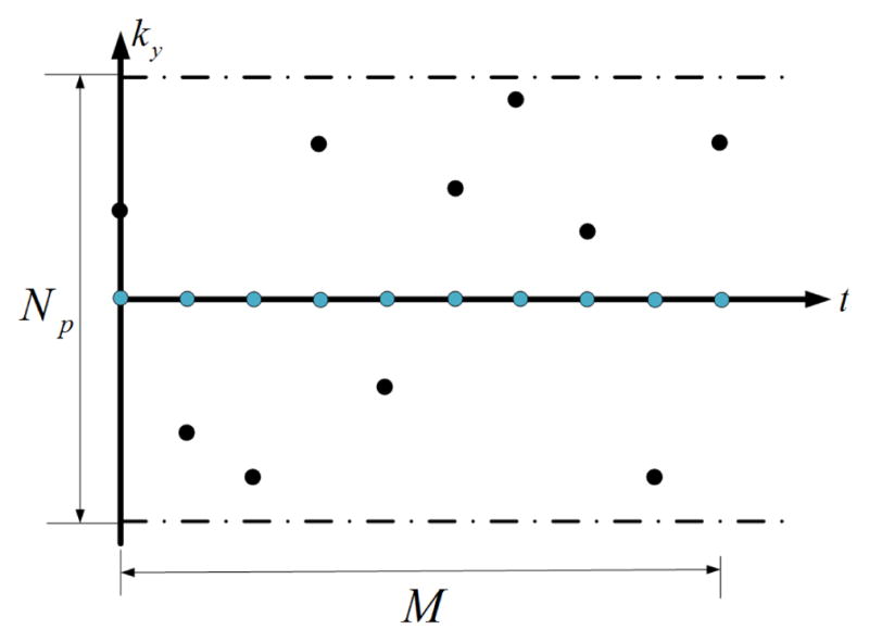
Data acquisition scheme in the simulation. Blue dots represent the training data, while black dots represent the imaging data.
In addition to the proposed method (order-16 PSF with sparsity constraint), two other reconstruction methods were applied to process this data: order-6 PSF (the best-performing basic PSF method for the data set tested) and ℓ1-regularized reconstruction without PSF modeling [10]. For both methods including ℓ1-regularization, the regularization parameters were chosen manually to optimize the performance.
Some representative snapshot images reconstructed from the human and rat data sets (zoomed-in to the heart) are shown in Fig. 3 and 4, respectively. It is clear that the proposed method has a much better spatial resolution than the other two methods, particularly in the myocardium and the blood pool, where the other two methods produced significant artifacts. Relative reconstruction error defined as, i.e.,
Fig. 3.
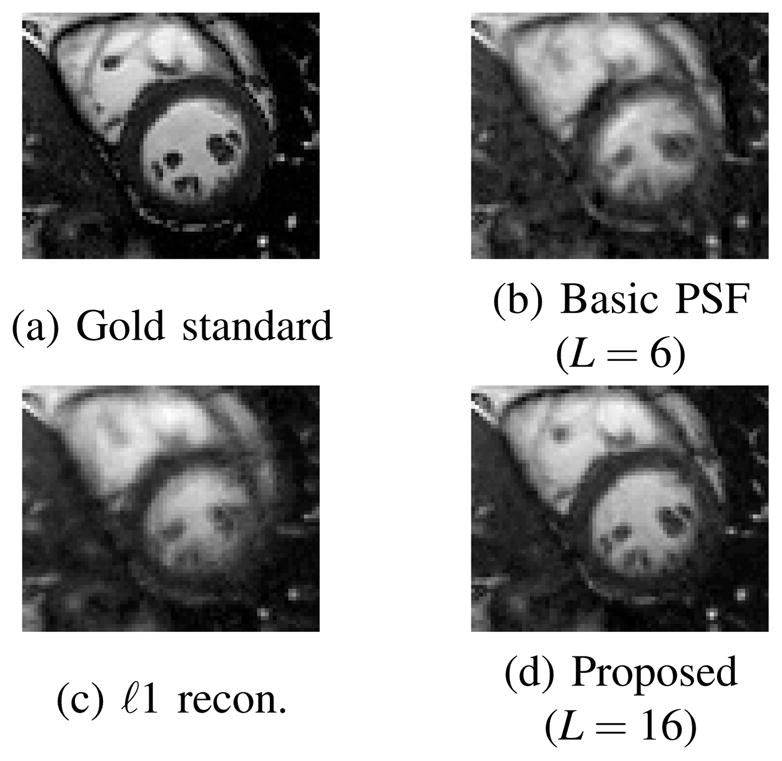
Reconstructions of the human phantom (zoomed-in to the heart) using 11 data frames.
Fig. 4.
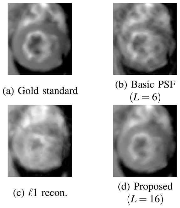
Reconstructions of the rat phantom (zoomed-in to the heart) using 11 data frames.
| (17) |
are shown in Table I, which are consistent with the improved performance of the proposed method.
TABLE I.
Relative reconstruction errors.
| Phantom | Order-6 PSF | ℓ1 recon. | Proposed |
|---|---|---|---|
| Human | 6.45% | 5.98% | 4.01% |
| Rat | 4.94% | 6.90% | 2.10% |
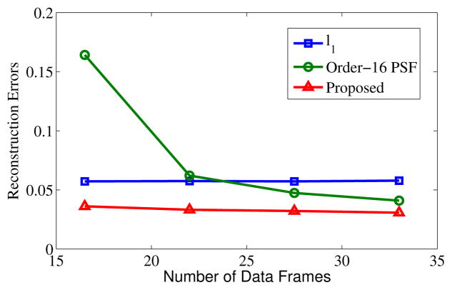
Tests were also done to compare the amount of data required for (a) ℓ1 regularized reconstruction without PSF modeling, (b) basic PSF with L = 16, and (c) the proposed method with L = 16. Reconstruction errors as a function of the amount of acquired data are shown in Fig. 5, and reconstructed images are shown in Fig. 6. As expected, reconstruction performance improves with the increasing data for both basic PSF and the proposed method. However, the proposed method can reconstruct higher quality images especially when the number of data frames is small compared with the basic PSF with the same model order. For ℓ1 regularized reconstruction without PSF modeling, the reconstructed images suffer from significant blurring artifacts although the reconstructions are stable with different amount of measurements.
Fig. 5.
Reconstruction errors versus the number of data frames for the human phantom. The errors for ℓ1 regularized reconstruction almost do not change with the increasing amount of data. Basic PSF reconstruction needs a large amount of measured data for accurate reconstruction, while the proposed method can yield high-quality reconstructions with much less data.
Fig. 6.
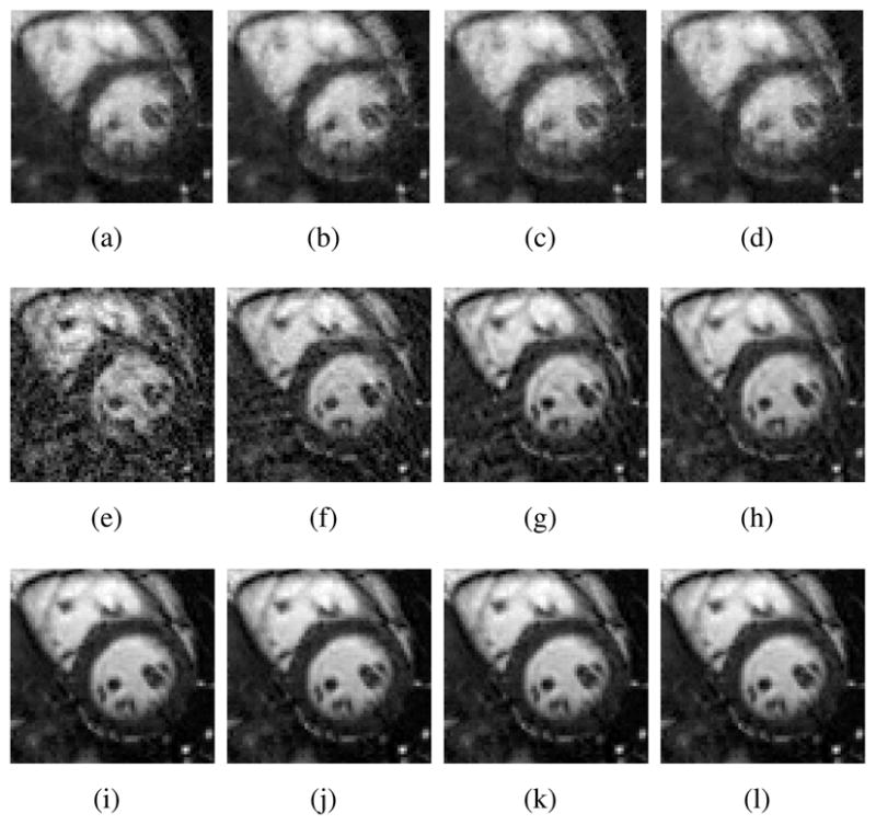
Reconstructions of the human phantom (zoomed-in to the heart). (a)–(d) show ℓ1 regularized reconstructions without PSF modeling using 16.5, 22, 27.5, 33 data frames, respectively; (e)–(h) show basic order-16 basic PSF reconstructions using 16.5, 22, 27.5, and 33 data frames, respectively; (i)–(l) show reconstructions with the proposed method (order-16 PSF with sparsity constraint) using 16.5, 22, 27.5, and 33 data frames, respectively.
B. Discussion
Simultaneous use of rank and sparsity constraints was also considered in [11]. Instead of imposing an explicit rank constraint, the algorithm in [11] minimizes the nuclear norm. We have observed that the explicit rank constraint can be more effective than the nuclear norm rank constraint [18]. In terms of computation, the proposed algorithm has the following advantages over the ℓ1 and nuclear norm minimization algorithm. The algorithm in [11] requires one SVD (or partial SVD) at each iteration, which is much more time-consuming than solving the decoupled least squares problems in (16). In addtion, for the proposed method both spatial and temporal Fourier transforms can be computed on the spatial and temporal basis, instead of the whole data matrix, which is more efficient.
IV. Conclusion
A new method has been described for reconstruction of highly undersampled (k, t)-space data. This method simultaneously enforces partial separability (low-rankness) and encourages sparsity in the (x, f)-domain. The resulting reconstruction problem is efficiently solved using an additive half-quadratic optimization procedure. The proposed method has been validated with simulated data, and shows significantly better performance than the existing methods that use rank or sparsity constraints alone.
Acknowledgments
This work was supported in part by the following research grants: NIHP41-EB-00197, NIH-P41-RR-02395, and NSF-CBET-07-30623.
References
- 1.Liang ZP, Jiang H, Hess CP, Lauterbur PC. Dynamic imaging by model estimation. Int J Imaging Syst Tech. 1997;8:551–557. [Google Scholar]
- 2.Tsao J, Boesiger P, Pruessmann KP. k-t BLAST and k-t SENSE: Dynamic MRI with high frame rate exploring spatiotemporal sparsity. Magn Reson Med. 2003;50:1031–1042. doi: 10.1002/mrm.10611. [DOI] [PubMed] [Google Scholar]
- 3.Lustig M, Santos JM, Donoho DL, Pauly JM. k-t SPARSE: high frame rate dynamic mri exploiting spatio-temporal sparsity. Proc Int Symp Magn Reson Med. 2006:2420. [Google Scholar]
- 4.Liang ZP. Spatiotemporal imaging with partially separable functions. Proc IEEE Int Symp Biomed Imaging. 2007:988–991. [Google Scholar]
- 5.Aggarwal N, Bresler Y. Patient-adapted reconstruction and acquisition dynamic imaging method (PARADIGM) for MRI. Inverse Probl. 2008;24:045015. [Google Scholar]
- 6.Brinegar C, Wu YJL, Foley LM, Hitchens TK, Ye Q, Ho C, Liang ZP. Real-time cardiac MRI without triggering, gating, or breath holding. Proc IEEE Eng Med Bio Conf. 2008:3381–3384. doi: 10.1109/IEMBS.2008.4649931. [DOI] [PMC free article] [PubMed] [Google Scholar]
- 7.Brinegar C, Zhang H, Wu YJL, Foley LM, Hitchens TK, Ye Q, Pocci D, Lam F, Ho C, Liang ZP. Real-time cardiac MRI using prior spatial-spectral information. Proc IEEE Eng Med Bio Conf. 2009:4383–4386. doi: 10.1109/IEMBS.2009.5333482. [DOI] [PMC free article] [PubMed] [Google Scholar]
- 8.Christodoulou AG, Brinegar C, Haldar JP, Zhang H, Wu YJL, Foley LM, Hitchens TK, Ye CHQ, Liang ZP. High-resolution cardiac MRI using partially separable functions and weighted spatial smoothness regularization. Proc IEEE Eng Med Bio Conf. 2010 doi: 10.1109/IEMBS.2010.5627889. to be published. [DOI] [PMC free article] [PubMed] [Google Scholar]
- 9.Gamper U, Boesiger P, Kozerke S. Compressed sensing in dynamic MRI. Magn Reson Med. 2008:365–373. doi: 10.1002/mrm.21477. [DOI] [PubMed] [Google Scholar]
- 10.Jung H, Sung K, Nayak KS, Kim EY, Ye JC. k-t FOCUSS: a general framework for high resolution dynamic MRI. Magn Reson Med. 2009:103–116. doi: 10.1002/mrm.21757. [DOI] [PubMed] [Google Scholar]
- 11.Goud S, Hu Y, Jacob M. Real-time cardaic MRI using low rank and sparsity penalties. Proc IEEE Int Symp Biomed Imaging. 2010:988–991. [Google Scholar]
- 12.Donoho DL. Compressed sensing. IEEE Trans Inf Theory. 2006;52(4):1289–1306. [Google Scholar]
- 13.Geman D, Yang C. Nonlinear image recovery with half-quadratic regularization. IEEE Trans Image Process. 1995;4(7):932–946. doi: 10.1109/83.392335. [DOI] [PubMed] [Google Scholar]
- 14.Nikolova M, Ng M. Analysis of half-quadratic minimization methods for signal and image recovery. SIAM J Sci Comput. 2005;27(3):937–965. [Google Scholar]
- 15.Madsen K, Bruun H. A finite smoothing algorithm for linear ℓ1 estimation. SIAM J Optimization. 1993;3(2):223–225. [Google Scholar]
- 16.Becker S, Bobin J, Candès EJ. NESTA: A fast and accurate first-order method for sparse recovery. Preprint. 2009 http://arxiv.org/abs/0904.3367.
- 17.Björck Å. Numerical methods for least squares problems. Philadephia, PA: SIAM; 1996. [Google Scholar]
- 18.Haldar JP, Hernando D. Rank-constrained solutions to linear matrix equations using PowerFactorization. IEEE Signal Process Lett. 2009;16:584–587. doi: 10.1109/LSP.2009.2018223. [DOI] [PMC free article] [PubMed] [Google Scholar]


