Clinicians' Guide to Statistics for Medical Practice and Research: Part I

Introduction

This two-part series will present basic statistical principles for the practicing physician to use in his or her review of the literature and to the physician engaged in clinical research. The purpose of this series is threefold: (1) to provide an overview of common epidemiological and statistical terms and concepts that can be useful to the practitioner and clinical researcher, (2) to review calculations for common epidemiological measures and statistical tests, and (3) to provide examples from the published literature of uses of statistics in medical care and research. This review is not intended to be a comprehensive presentation of epidemiology or statistics since there are already a number of excellent sources for this information 1–6), but rather as a quick reference for practical application of statistical principles and concepts in medical care and clinical research.

In this issue, Part I of the Series is presented and includes discussion of the study question, study goals, appropriate study design, and appropriate statistical tests.

Physicians can be overwhelmed when reviewing published and current studies to determine what is relevant to their clinical practice and/or clinical research. Some initial questions outlined below may guide the process for reviewing an article or setting up a clinical study.

• What is the study question? What are the study goals?

• What is the appropriate study design to answer the study question?

• What are the appropriate statistical tests to utilize?

What Is the Study Question? What Are the Study Goals?

Whether in clinical practice or in a clinical research “laboratory,” physicians often make observations that lead to questions about a particular exposure and a specific disease. For example, one might observe in clinical practice that several patients taking a certain antihypertensive therapy develop pulmonary symptoms within 2 weeks of taking the drug. The physician might question if the antihypertensive therapy is associated with these symptoms. A cardiologist may observe in a review of the medical literature that the initial costs of caring for patients with cardiovascular diseases have been reported to be greater if the patient is cared for by a specialist than if the patient is cared for by a non-specialist. Because the physician may believe that although initial costs are greater, the follow-up costs are less, he or she may question if there would be a difference by specialist versus non-specialist if all costs were assessed. Questions like these can lead to formal hypotheses that can then be tested with appropriate research study designs and analytic methods. Identifying the study question or hypothesis is a critical first step in planning a study or reviewing the medical literature. It is also important to understand up front what the related study goals are. Some questions that may facilitate the process of identifying the study goals follow:

• Is the goal to determine:

• – how well a drug or device works under ideal conditions (i.e., efficacy)?

• – how well a drug or device works in a free-living population (i.e., effectiveness)?

• – the causes or risk factors for a disease?

• – the burden of a disease in the community?

• Is the study goal to provide information for a quality management activity?

• Will the study explore cost-effectiveness of a particular treatment or diagnostic tool? The hypotheses and the goals of a study are the keys to determining the study design and statistical tests that are most appropriate to use.

What Is the Appropriate Study Design To Answer the Study Question?

Once the study question(s) and goals have been identified, it is important to select the appropriate study design. Although the key classification scheme utilizes descriptive and analytic terminology, other terminology is also in vogue in evaluating health services and will be briefly described at the end of this section.

Classification Schemes

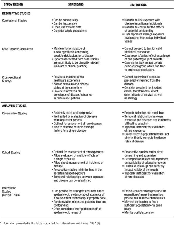
Epidemiology has been defined as “the study of the distribution and determinants of disease frequency” in human populations (4). The primary classification scheme of epidemiological studies distinguishes between descriptive and analytic studies. Descriptive epidemiology focuses on the distribution of disease by populations, by geographic locations, and by frequency over time. Analytic epidemiology is concerned with the determinants, or etiology, of disease and tests the hypotheses generated from descriptive studies. Table 1 lists the study design strategies for descriptive and analytic studies. Below is a brief description of the various design strategies. The strengths and limitations of these study designs are compared in Table 2.

Table 1: Outline of Study Design Strategies for Descriptive and Analytic Studies.

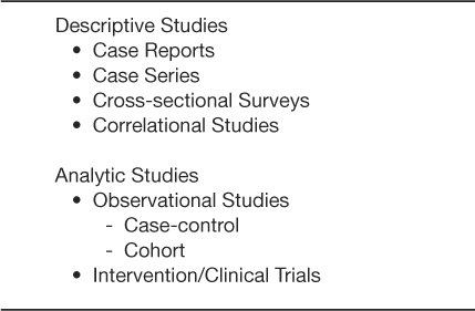
Table 2: Strengths and Limitations of Descriptive and Analytic Study Designs*

Descriptive Studies:

Correlational studies, also called ecologic studies, employ measures that represent characteristics of entire populations to describe a given disease in relation to some variable of interest (e.g. medication use, age, healthcare utilization). A correlation coefficient (i.e. Pearson's “r”; Spearman's “T”; or Kendall's “K”) quantifies the extent to which there is a linear relationship between the exposure of interest or “predictor” and the disease or “outcome” being studied. The value of the coefficient ranges between positive 1 and negative 1. Positive 1 reflects a perfect correlation where as the predictor increases, the outcome (or risk of outcome) increases. Negative 1 reflects a perfect inverse correlation where as the predictor increases the outcome (or risk of outcome) decreases. An example of a correlation study would be that of St Leger and colleagues who studied the relationship between mean wine consumption and ischemic heart disease mortality (7). Across 18 developed countries, a strong inverse relationship was present. Specifically, countries with higher wine consumption had lower rates of ischemic heart disease and countries with lower wine consumption had higher rates of ischemic heart disease. Although correlation studies provide an indication of a relationship between an exposure and an outcome, this study design does not tell us whether people who consume high quantities of wine are protected from heart disease. Thus, inferences from correlation studies are limited.

Case reports and case series are commonly published and describe the experience of a unique patient or series of patients with similar diagnoses. A key limitation of the case report and case series study design is the lack of a comparison group. Nonetheless, these study designs are often useful in the recognition of new diseases and formulation of hypotheses concerning possible risk factors. In a case series study reported by Kwon and colleagues (8), 47 patients were examined who developed new or worsening heart failure during treatment with tumor necrosis factor (TNF) antagonist therapy for inflammatory bowel disease or rheumatoid arthritis. After TNF antagonist therapy, 38 patients (of which 50% had no identifiable risk factors) developed new-onset heart failure and 9 experienced heart failure exacerbation. From this descriptive study, the authors concluded that TNF antagonist might induce new-onset heart failure or exacerbate existing disease (8).

Cross-sectional surveys are also known as prevalence surveys. In this type of study, both exposure and disease status are assessed at the same time among persons in a well-defined population. These types of studies have become more common recently with the development and validation of survey tools such as the Short Form 36 (SF 36) functional status questionnaire and the Kansas City Cardiomyopathy Questionnaire (KCCQ) functional status survey. Cross-sectional studies are especially useful for estimating the population burden of disease. The prevalence of many chronic diseases in the United States is calculated using the National Health and Nutrition Examination Survey, an interview and physical examination study including thousands of non-institutionalized citizens of the United States. For example, Ford and colleagues estimated that 47 million Americans have the metabolic syndrome using the Third National Health and Nutrition Examination Survey (9). Of note, in special circumstances where one can easily deduce an exposure variable preceding the outcome or disease, cross sectional surveys can be used to test epidemiologic hypotheses and thus can be used as an analytic study. For example, Bazzano and colleagues used data collected from a cross-sectional study to conclude that cigarette smoking may raise levels of serum C-reactive protein (10). A cross-sectional study is useful in this situation because it is unlikely that having high levels of C-reactive protein would cause one to smoke cigarettes.

Analytic Studies:

Analytic studies can be observational or experimental. In observational studies, the researchers record participants' exposures (e.g., smoking status, cholesterol level) and outcomes (e.g., having a myocardial infarction). In contrast, an experimental study involves assigning one group of patients to one treatment and another group of patients to a different or no treatment. There are two fundamental types of observational studies: case control and cohort. A case control study is one in which participants are chosen based on whether they do (cases) or do not (controls) have the disease of interest. Ideally, cases should be representative of all persons developing the disease and controls representative of all persons without the disease. The cases and controls are then compared as to whether or not they have the exposure of interest. The difference in the prevalence of exposure between the disease/no disease groups can be tested. In these types of studies, the odds ratio is the appropriate statistical measure that reflects the differences in exposure between the groups.

The defining characteristic of a cohort study, also known as a follow-up study, is the observation of a group of participants over a period of time during which outcomes (e.g., disease or death) develop. Participants must be free from the disease of interest at the initiation of the study. Subsequently, eligible participants are followed over a period of time to assess the occurrence of the disease or outcome. These studies may be classified as non-concurrent/retrospective or concurrent/prospective.

Retrospective cohort studies refer to those in which all pertinent events (both exposure and disease) have already occurred at the time the study has begun. The study investigators rely on previously collected data on exposure and disease. An example of a non-concurrent/retrospective cohort study would be that of Vupputuri and colleagues (11), who in 1999–2000 abstracted data on blood pressure and renal function from charts for all patients seen at the Veterans Administration Medical Center of New Orleans Hypertension Clinic from 1976 through 1999. They analyzed the data to see if blood pressure at each patient's first hypertension clinic encounter was associated with a subsequent deterioration in renal function.

In prospective studies, the disease/outcome has not yet occurred. The study investigator must follow participants into the future to assess any difference in the incidence of the disease/outcome between the types of exposure. The incidence of the disease/outcome is compared between the exposed and unexposed groups using a relative risk (RR) calculation. The advantages of retrospective cohort studies, relative to prospective, include reduced cost and time expenditures as all outcomes have already occurred. In contrast, the major disadvantage of the non-concurrent/retrospective studies is the reliance on available data that were collected for clinical purposes and, generally, not following a carefully designed protocol. There are two additional sub-classifications for cohort studies. First, cohort studies may include a random sample of the general population, e.g., Framingham and Atherosclerosis Risk in Communities (12–16) or a random sample of a high-risk population (17). In these latter studies, a sample of all individuals or individuals with a specific demographic, geographic, or clinical characteristic is included. Second, cohort studies may begin by identifying a group of persons with an exposure and a comparison group without the exposure. This type of cohort study is usually performed in the situation of a rare exposure.

Experimental or intervention studies are commonly referred to as clinical trials. In these studies, participants are randomly assigned to an exposure (such as a drug, device, or procedure). “The primary advantage of this feature (ed: randomized controlled trials) is that if the treatments are allocated at random in a sample of sufficiently large size, intervention studies have the potential to provide a degree of assurance about the validity of a result that is simply not possible with any observational design option” (5). Experimental studies are generally considered either therapeutic or preventive. Therapeutic trials target patients with a particular disease to determine the ability of a treatment to reduce symptoms, prevent recurrence or decrease risk of death from the disorder. Prevention trials involve the assessment of particular therapies on reducing the development of disease in participants without the disease at the time of enrollment. One such prevention trial is the Drugs and Evidence Based Medicine in the Elderly (DEBATE) Study, which has as its primary aim “ to assess the effect of multi-factorial prevention on composite major cardiovascular events in elderly patients with atherosclerotic diseases” (18).

Other Classification Schemes:

Some other classification schemes in use today are based on the use of epidemiology to evaluate health services. Epidemiological and statistical principles and methodologies are used to assess health care outcomes and services and provide the foundation for evidence-based medicine. There are different ways to classify studies that evaluate health care services. One such scheme distinguishes between process and outcomes studies. Process studies assess whether what is done in the medical care encounters constitutes quality care (e.g. number and type of laboratory tests ordered, number and type of medications prescribed, frequency of blood pressure measurement). An example of a process study would be one that evaluated the percentage of patients with chronic heart failure in a given population who have filled prescriptions for angiotensin converting enzyme inhibitors (ACE – Inhibitors). A criticism of process studies is that although they document whether or not appropriate processes were done, they don't indicate if the patient actually benefited or had a positive outcome as a result of the medical processes.

Outcomes studies assess the actual effect on the patient (e.g. morbidity, mortality, functional ability, satisfaction, return to work or school) over time, as a result of their encounter(s) with health care processes and systems. An example of this type of study would be one that assessed the percentage of patients with a myocardial infarction (MI) who were placed on a beta blocker medication and subsequently had another MI. For some diseases, there may be a significant time lag between the process event and the outcome of interest. This often results in some patients being lost to follow-up, which may lead to erroneous conclusions unless methods that “censor” or otherwise adjust for missing time-dependent covariates are used.

In reviewing the medical literature, one often encounters other terms that deal with the evaluation of medical services: efficacy, effectiveness, or efficiency. Efficacy evaluates how well a test, medication, program or procedure works in an experimental or “ideal” situation. Efficacy is determined with randomized controlled clinical trials where the eligible study participants are randomly assigned to a treatment or non-treatment, or treatment 1 versus treatment 2, group. Effectiveness assesses how well a test, medication, program or procedure works under usual circumstances. In other words, effectiveness determines to what extent a specific healthcare intervention does what it is intended to do when applied to the general population. For example, although certain anti-retroviral therapies work well using direct observed therapy in the controlled setting of a clinical trial (i.e., they are efficacious), once applied to a free-living population, the drug dosing regimen may be too difficult for patients to follow in order to be effective. Finally, efficiency evaluates the costs and benefits of a medical intervention.

What Are the Appropriate Statistical Tests?

Once the appropriate design is determined for a particular study question, it is important to consider the appropriate statistical tests that must be (or have been) performed on the data collected. This is relevant whether one is reviewing a scientific article or planning a clinical study. To begin, we will look at terms and calculations that are used primarily to describe measures of central tendency and dispersion. These measures are important in understanding key aspects of any given dataset.

Measures of Central Tendency

There are three commonly referred to measures of central location: mean, median, and mode. The arithmetic mean or average is calculated by summing the values of the observations in the sample and then dividing the sum by the number of observations in the sample. This measure is frequently reported for continuous variables: age, blood pressure, pulse, body mass index (BMI), to name a few. The median is the value of the central observation after all of the observations have been ordered from least to greatest. It is most useful for ordinal or non-normally distributed data. For data sets with an odd number of observations, we would determine the central observation with the following formula:

For datasets with an even number of observations, we would select the case that was the average of the following observations' values:

The mode is the most commonly occurring value among all the observations in the dataset. There can be more than one mode. The mode is most useful in nominal or categorical data. Typically no more than two (bimodal) are described for any given dataset.

Example 1: A patient records his systolic blood pressure every day for one week. The values he records are as follows: Day 1: 98 mmHg, Day 2: 140 mmHg, Day 3: 130 mmHg, Day 4: 120 mmHg, Day 5: 130 mmHg, Day 6: 102 mmHg, Day 7: 160 mmHg.

The arithmetic mean or average for these 7 observations is calculated as follows:

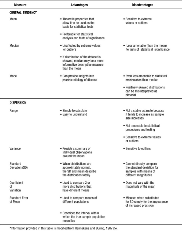
In calculating the median, the values must be ordered from least to greatest: 98, 102, 120, 130, 130, 140, 160. There are 7 observations in this dataset, an odd number. Therefore, the formula is used to determine that the fourth observation will be the median. The value of the fourth observation is 130 mmHg. Therefore, the median is 130 mmHg. In the example, the mode is also 130 mmHg. This is the only value that occurs more than once; hence it is the most commonly occurring value. Investigators and practitioners are often confused which measure of centrality is most relevant to a given dataset. Table 3 outlines key advantages and disadvantages to the choice of measure of central location. It is interesting to note that if the dataset consists of continuous variables with unimodal and symmetric distribution, then the mean, median, and mode are the same.

Table 3: Advantaged and Disadvantages of Measure of Central Tendency and Dispersion*

Measures of Dispersion

Measures of dispersion or variability provide information regarding the relative position of other data points in the sample. Such measures include the following: range, inter-quartile range, standard deviation, standard error of the mean (SEM), and the coefficient of variation.

Range is a simple descriptive measure of variability. It is calculated by subtracting the lowest observed value from the highest. Using the blood pressure data in example 1, the range of blood pressure would be 160 mmHg minus 98 mmHg or 62 mmHg. Often given with the median (i.e., for non-normally distributed data) is the interquartile range, which reflects the values for the observations at the 25th and 75th percentiles of a distribution.

The most commonly used measures of dispersion include variance and its related function, standard deviation, both of which provide a summary of variability around the mean. Variance is calculated as the sum of the squared deviations divided by the total number of observations minus one:

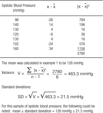
The standard deviation is the square root of the variance. Table 4 presents calculations of variance and standard deviation for the systolic blood pressures given in example 1.

Table 4: Example of a Standard Deviation Calculation

The coefficient of variation (CV) is a measure that expresses the SD as a proportion of the mean:

This measure is useful if the clinician wants to compare 2 distributions that have means of very different magnitudes. From the data provided in example 1, the coefficient of variation would be calculated as follows:

The standard error of the mean (SEM) measures the dispersion of the mean of a sample as an estimate of the true value of the population mean from which the sample was drawn. It is related to, but different from, the standard deviation. The formula is as follows:

Using the data from example 1, the SEM would be:

SEM can be used to describe an interval within which the true sample population mean lies, with a given level of certainty. Which measure of dispersion to use is dependent on the study purpose. Table 3 provides some information which may facilitate the selection of the appropriate measure or measures.

Comparing Central Tendencies with Respect to Dispersions (Error Terms)

Once central tendency and dispersion are measured, it follows that a comparison between various groups (e.g., level of systolic blood pressure among persons taking ACE-Inhibitors versus beta-blockers) is desired. If working with continuous variables that are normally distributed, the comparison is between means. The first step is to simply look at the means and see which is larger (or smaller) and how much difference lies between the two. This step is the basis of deductive inference. In comparing the means, and, preferably before calculating any p-values, the clinician or investigator must answer the question: is the observed difference clinically important? If the magnitude of the observed difference is not clinically important, then the statistical significance becomes irrelevant in most cases. If the observed difference is clinically important, even without statistical significance, the finding may be important and should be pursued (perhaps with a larger and better powered study; Table 5).

Table 5.

Clinical Versus Statistical Significance and Possible Conclusions

Once a deductive inference is made on the magnitude of the observed differences, statistical inference follows to validate or invalidate the conclusion from the deductive inference. To illustrate: if two people each threw one dart at a dartboard, would one conclude that whoever landed closer to the center was the more skilled dart thrower? No. Such a conclusion would not be reasonable even after one game or one match as the result may be due to chance. Concluding who is a better player would have to be based on many games, against many players, and over a period of time. There are many reasons for inconsistencies (good day, bad day, etc.), but they all boil down to variance. For a player to be classified as a “good player,” he/she has to be consistently good over time.

Because in clinical research we rely on a sample of the patient population, variance is a key consideration in the evaluation of observed differences. The observed difference between exposed and unexposed groups can be large, but one must consider how it stands next to the variation in the data. Since these parameters are highly quantifiable, the probability that the means are different (or similar) can be calculated. This process takes place in a statistical method called analysis of variance (ANOVA). The details of this process are beyond the scope of this chapter; nevertheless, ANOVA is a fundamental statistical methodology and is found in many texts and is performed by many statistical software packages. In essence, the ANOVA answers the question: are differences between the study groups' mean values substantial relative to the overall variance (all groups together)? It is important to note that even though ANOVA reveals statistically significant differences, the ANOVA does not indicate between which groups the difference exists. Therefore, further analysis with multiple comparison tests must be performed to determine which means are significantly different. Portney and Watkins (19) provide a good overview of these procedures.

In the special case where one and only one comparison can be made, the t-test can be done. It was developed to be a shortcut comparison of only two means between groups with small sample sizes (less than 30). If used for more than one comparison or when more than one comparison is possible, the t-tests do not protect against Type 1 error at the assumed level of tolerance for Type 1 error (usually α = 0.05).

Probability: Fundamental Concepts in Evidence-Based Medicine

Armed with a basic understanding of algebra and user-friendly statistical software, most clinicians and clinical researchers can follow the cookbook method of statistical inference. Problems quickly arise because the vast majority of medical research is not designed as simply as the examples given in basic statistics textbooks nor analyzed as simply as the shortcut methods often programmed beneath the layers of menus in easy-to-use software. Violations of assumptions that are necessary for a classic statistical method to be valid are more the rule than the exception. However, avoiding the misinterpretation of statistical conclusions does not require advanced mastery of the mathematics of probability at the level of calculus. An effort to understand, at least qualitatively, how to measure the degree of belief that an event will occur will go a long way in allowing non-mathematicians to make confident conclusions with valid methods.

Two practical concepts should be understood up front: first, understanding that every probability, or rate, has a quantifiable uncertainty that is usually expressed as a range or confidence interval. Second, that comparing different rates observed between two populations, or groups, must be done relative to the error terms. This is the essence of statistical inference.

Probability Distributions:

The final rate of an event that is measured, as the size of the sample being measured grows to include the entire population, is the probability that any individual in the population will experience the event. For example, one analyzes a database of heart transplant patients who received hearts from donors over the age of 35 to determine the rate of cardiac death within a 5-year post-transplant follow-up period (20). If the first patient in the sample did not survive the study period, the sample of this one patient gives an estimated cardiac death rate of 100%. No one would accept an estimate from a sample of one. However, as the sample size increases, the event rate will migrate towards truth. If the next patient in the database is a survivor, the cardiac death rate falls to 50%. Once the entire population represented in the database is included in the sample (n=26), it is observed that 7 experienced cardiac death for a final cardiac death rate of 27%. When written as a probability, one can say that the probability is 0.27 that any single participant randomly sampled from this database will be recorded as having a cardiac death within 5 years of receiving a heart transplant. It may be more relevant to use the data to predict that the next patient seen in clinic and added to the database will have a probability of 0.27 of experiencing cardiac death within 5 years. The illustration just described is that of a binomial probability. That is, the outcome is one of two possible levels (binary): survival or death.

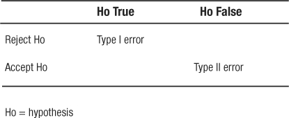
To complete the estimate of a probability of an event in this population, a measure of uncertainty must be placed around this point estimate. In this case, the standard error (SE, not to be confused with the SEM described earlier) is calculated with the classic formula . This formula indicates that the square root of the function of the probability of event (p), times the probability of no event (1-p), divided by the sample size (n) is the standard error (SE) of the event rate. The SE multiplied by the Z score of the tolerance for Type I error is one-half of the range for a confidence interval of the same tolerance for Type I error (Note: for information regarding Type I error, see section on “Are the results of the study significant?”).

For this example, the SE is calculated by:

The Z score for a two sided 95% confidence interval (CI) is 1.96, so the range of the CI is calculated by lower 95% CI = 0.27 − 1.96 × 0.087 = 0.011 and upper 95% CI = 0.27 + 1.96 × 0.087 = 0.440, respectively. These yield the range (.011, .440). Thus, if this observation were repeated 100 times in similar populations of the same sample size, 95 of the sampled death rates would fall between .011 and .440.

Evaluating Diagnostic and Screening Tests

In order to understand disease etiology and to provide appropriate and effective health care for persons with a given disease, it is essential to distinguish between persons in the population who do and do not have the disease of interest. Typically, we rely on screening and diagnostic tests that are available in medical facilities to provide us information regarding the disease status of our patients. However, it is important to assess the quality of these tests in order to make reasonable decisions regarding their interpretation and use in clinical decision-making (1). In evaluating the quality of diagnostic and screening tests, it is important to consider the validity (i.e. sensitivity and specificity) as well as the predictive value (i.e. positive and negative predictive values) of the test.

Sensitivity is the probability (Pr) that a person will test positive (T+) given that they have the disease (D+). Specificity is the probability (Pr) that a person will test negative (T−) given that they do not have the disease (D−). These are conditional probabilities. The result in question is the accuracy of the test, and the condition is the true, yet unknown, presence or absence of the disease. Sensitivity and specificity are properties of the screening test, and, like physical properties, follow the test wherever it is used. They can be useful in determining the clinical utility of the test (as a screening tool vs. a diagnostic tool) as well as comparing new tests to existing tests. They are written mathematically as:

It is more common for sensitivity and specificity to be expressed from a 2×2 contingency table (Table 6) as follows:

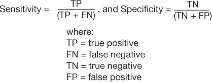Table 6: 2×2 Contigency Table – Test Characteristics

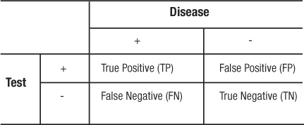
These parameters quantify the validity of a test when it is evaluated in a population that represents the spectrum of patients in whom it would be logical and clinically useful to use the test. The most obvious limitation of evaluating a screening test is identifying an optimal gold standard to determine the disease status. In the evaluation of new screening tests, existing tests are often used as the gold standard. Disagreement or poor sensitivity and specificity of the new test could mean that the new test does not work as well as, or that it is actually superior to, the existing test. A histological test from a biopsy is the least disputable gold standard. Nonetheless, the limitation with regards to the gold standard is unavoidable and must be recognized in the continuous evaluation of clinical screening and diagnostic testing.

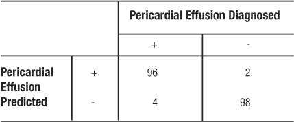
In a study to evaluate bedside echocardiography by emergency physicians to detect pericardial effusion, 478 eligible patients were evaluated for the condition both by the emergency department physician and by the cardiologist (who had the clinical responsibility to make the diagnosis); the cardiologist's finding was used as the gold standard (21).

An excerpt of the results is shown in Table 7. From the data presented in the table, the following can be calculated:

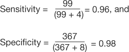Table 7: 2×2 Contingency Table for Pericardial Effusion Study

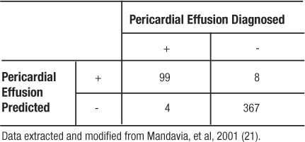
Since the sensitivity and specificity are like physical properties of the test, we can determine the portion of TP and TN regardless of the prevalence of the disease in the population studied. For example, if we had recruited 100 patients with pericardial effusion and 100 matching participants without pericardial effusion, the resulting table would yield the same rates of TP, TN, and identical values for sensitivity and specificity (Table 8).

Table 8: 2×2 Contingency Table for Pericardial Effusion Example

Positive predictive value (PPV) is the probability (Pr) that the disease is truly present (D+) given that the test result is positive (T+). Negative predictive value (NPV) is the probability that the disease is truly absent (D−) given that the test result is negative (T−). Generally speaking, patients (and their physicians) are more concerned with these probabilities. These are also conditional probabilities. These parameters are written mathematically as:

PPV = Pr(D⁺|T⁺), and NPV = Pr(D⁻|T⁻). As with sensitivity and specificity, it may be more common to see the algebraic expressions:

The question is whether or not the individual patient's test result is true. Unlike sensitivity and specificity, PPV and NPV are dependent upon the prevalence of the disease in the population. The example below further illustrates this point.

In the study by Mandavia et al, 103 patients were diagnosed as having a pericardial effusion out of 478 eligible patients (21). This study population has a prevalence of pericardial effusion of (Table 7). However, the pericardial effusion example (Table 8) using case-matched controls artificially fixed the prevalence to 50%. In the original study, , and (Table 7). However, in the example using the case-control design with 50% of the study population with disease, , and (Table 8). The comparison of these values illustrates that PPV increases with prevalence (is directly proportional) and NPV decreases with prevalence (is inversely proportional).

Figure 1 shows PPV and NPV over the entire range of possible prevalence with sensitivity and specificity fixed at the values in the illustration. PPV and NPV are used to make clinical decisions concerning an individual patient based on the population from which the patient comes. As prevalence increases, PPV increases and NPV decreases. Thus, in populations where disease prevalence is high, there will be greater confidence that a positive test result is a true positive, and increased suspicion that a negative test result is a false negative. The reverse is true in populations where the disease prevalence is low (e.g. rare disease).

Diagnostic and screening tests, and their related sensitivities, specificities, PPVs and NPVs, facilitate the clinician's classification of a patient with regard to a specific disease status. The ultimate goal of the diagnostic process is to establish a diagnosis with sufficient confidence to justify treatment or to exclude a diagnosis with sufficient confidence to justify non-treatment (22). In the process of determining a diagnosis (or not), the test results for a given disease should be kept within the context of the probability of disease prior to receiving results. Bayesian logic is the understanding of conditional probability which is expressed mathematically in Baye's Theorem. The theorem “indicates that the result of any diagnostic test alters the probability of disease in the individual patient because each successive test result reclassifies the population from which the individual comes” (22).

Common Measures of Association and Statistical Tests

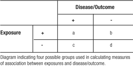
Measures of association are summary statistics that estimate the risk of an outcome or disease for a given exposure between two groups. Two frequently reported measures are the odds ratio and the relative risk. The odds ratio (OR) is calculated from a case-control study where the participants were selected by their outcome and then studied to determine exposure. Because the participants are selected on outcome, the case-control study reveals the prevalence of exposure among cases and controls. In case-control studies we calculate odds ratios because it is often a good estimate of the relative risk. Odds are the probability of an event occurring divided by the probability of the event not occurring. The OR ratio compares the odds of being exposed given a participant is a case (Table 9: a / a+c / c / a+c = a/c) relative to the odds of control participants being exposed (b/b+d / d / b+d = b/d). Using algebra to re-arrange the formula, the OR can be calculated as (Table 9):

Table 9: Cell Naming Scheme for Doing Calculations from a 2 × 2 Table

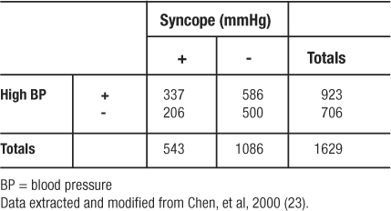
In an analysis from the Framingham Heart Study of risk factors for syncope, investigators identified 543 patients with a positive history of syncope (23). They then matched two controls (without a history of syncope) on age, gender, and follow-up time to every one case. (Using a case: control ratio of 1:2 is a strategy to increase statistical power of the analysis when the number of cases is limited.) Among other variables, they compared odds of high blood pressure (BP) between the syncope and non-syncope patients. Regarding high blood pressure prevalence in the two groups, Table 10 shows the findings. The OR was calculated to be indicating that having hypertension makes study participants 1.40 times more likely to experience syncope (be recorded as having a history of syncope) than those having normal BP.

Table 10: Diagram of Observed Frequencies Extracted for Odds Ratio Example

The relative risk or risk ratio (RR) is calculated from a cohort study where exposed and non-exposed participants are followed over time and the incidence of disease is observed. Because the hallmark of a cohort study is following a population over time to identify incident cases of disease, the cohort is screened to assure that no participant enrolled in the study has already experienced the outcome or disease event. Then, the cohort is followed for a specific period of time, and the incidence of events for the exposed and unexposed groups is measured. The relative risk can also be used to analyze clinical trial data. The relative risk (RR) is calculated from the labeled 2×2 table (Table 9) using the formula:

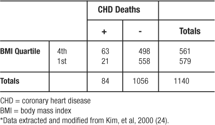
In another study from the Framingham Heart Study, investigators followed a cohort of 2373 women who were classified according to four categories of BMI (24). Over 24 years of follow-up, 468 women developed coronary heart disease (CHD); 150 of those women died from CHD (21 and 63 from the 1st and 4th quartiles of BMI, respectively). Regarding the incidence of CHD death in the 4th quartile of BMI versus the 1st quartile of BMI, the investigators observed the frequencies depicted in Table 11 (which omits the middle quartiles of BMI in order to illustrate the use of RR to analyze a 2×2 table from a cohort study). The , which means that persons in the 4th quartile BMI group have 3.10 times the risk of CHD related death compared to persons in the 1st quartile BMI group.

Table 11: Observed Frequencies Extracted from Relative Risk Example*

Both the OR and RR have confidence intervals (CI) as a measure of uncertainty. The method is similar to the one used for the binomial probability distribution. If a 95% CI excludes the value one (1), then the ratio is significant at the level of p<0.05. A test of independence, as a category of methods, tests the hypothesis that the proportion of an outcome is independent of the grouping category. The alternate hypothesis, the conclusion made when the p-value is significant (p<0.05), is that the disease or outcome is more common among the exposed or unexposed group.

Chi-square tests are used to determine the degree of belief that an observed frequency table could have occurred randomly by comparing it to an expected frequency table. The expected frequency table is derived based on the assumption that the row and column totals are true as observed and fixed. The most commonly used chi-square test is the Pearson's chi-square test. This is used to analyze a frequency table with two rows and two columns. When the table is not symmetrical or is of dimensions other than 2-by-2, the method is still valid, and when used is called the Cochran's chi-square test. At the very least, the largest observed difference is significant if the table is significant. If the overall table is significant, this global significance can allow stratified sub-analyses of the individual comparisons of interest. It can also be helpful to look at the contribution to the chi-square test statistic by each cell and conclude that the largest of these cells are where the observed frequencies most deviated from the expected frequencies.

If the chi-square tests on the tables for OR and RR result in p-values less than 0.05, then the 95% CI will also be significant. This being revealed, we are ready to illustrate how the chi-square test statistic is used to calculate the CI (2). The lower CI is calculated by exponentiation of the ratio with the value of the formula: where χ²_1,1-a is the value, from a look-up-table, of the chi-square test statistic that would set the maximum tolerance for Type 1 error, and X² is the chi-square test statistic from the observed table. The upper CI uses the same formula except by adding, rather than subtracting, the distance to the ratio: . The use of chi-square tables is covered in elementary texts on statistics, and the method for calculating the test is beyond the scope of this article. So as not to detract from emphasizing the principle of comparing the observed table to one expected, if the correlation were merely random we will simply state the values so the 95% CI for the OR and RR examples can be illustrated (Table 12). Thus, for the OR example, 1.40^0.36 = 1.12, and 1.40^1.64 = 1.73 resulted in an OR (95% CI) of 1.40 (1.12, 1.73). The CI range does not include 1 so the OR is statistically significant and validated the deductive inference that hypertension increases the odds of experiencing syncope. Similarly for the RR example, 3.10^.59 = 1.95, and 3.10^1.41 = 4.92 resulted in an RR (95% CI) of 3.10 (1.95, 4.92). The CI range does not include 1 so the RR is statistically significant and validated the deductive inference that higher BMI increases the risk of experiencing CHD death. Most often, the exposure is under study because it is considered harmful, so ratios greater than 1 and significant (by not including 1 in the range of the CI) are the more familiar result. However, ratios less than 1 and significant indicate that exposure is protective. An analysis from this viewpoint is helpful when the exposure is some behavior or event that is hypothesized to be therapeutic or helpful in building immunity.

Table 12: Components for Calculating a 95% Confidence Interval Around Measures of Association

Tests of proportional disagreement are for paired data, either repeated measures in the same participants or participants matched on demographic factors then given different exposures and followed to compare outcomes. The best known of the tests of proportional disagreement is the McNemar's chi-square test. The outcome of paired data falls into four observations (++, −–, +–, −+). McNemar's test focuses on the discordant cells (+–, −+) and tests the hypothesis that the disagreement is proportional between the two groups. If when the outcome disagrees, the disagreement is more frequently −+ than +–, then we know that more pairs are improving or having better outcomes. A relatively new application of tests for paired data is the Combined Quality Improvement Ratio (CQuIR), which uses the McNemar's chi-square test as the basis, but combines participants with repeated measures and case-control matched pairs into one large database of analyzable pairs. This process maximizes the statistical power available from the population (25, 26). Additionally, the ratio of discordant pairs (−+/+−) shows whether or not the disagreement is more often toward improvement. Included in the tests of disproportion is the Kappa statistic of agreement. The Kappa statistic evaluates the concordant cells (++ and −−) to conclude whether or not the agreement has enough momentum to be reproducible.

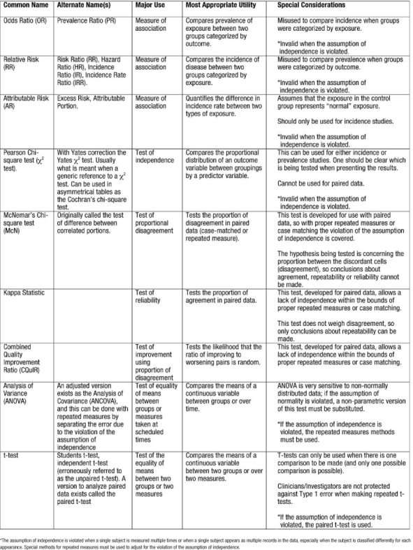
Thus far, we have used examples for analyses from observational studies. Experimental studies or clinical trials are analyzed in much the same manner. In clinical trials, patients are followed until some outcome is observed in the planned study period; these are incidence studies. As incidence studies, the RR will be the measure of association tested for statistical significance. Additionally, many clinical trials lend themselves to straightforward analyses with chi-square tests, ANOVA, or other methods that result only in a p-value. Table 13 summarizes common methods used to analyze healthcare data.

Table 13.

Measures of Association and Statistical Tests Commonly Used to Analyze Healthcare Data

For one example, we review the results of a trial of the beta-blocker, bucindolol, used in patients with advanced chronic heart failure (CHF) (27). While it is accepted that beta-blockers reduce morbidity and mortality in patients with mild to moderate CHF, these investigators enrolled 2708 patients designated as New York Heart Association (NYHA) class III or IV to test the efficacy of the beta-blocker in reducing morbidity and mortality in patients with high baseline severity. The primary outcome of interest was all-cause-mortality, which, being a relatively rare event, drove the sample size requirement to 2800 in order to statistically detect a clinically significant difference of 25%. Once enrolled, patients were randomly assigned to receive either placebo or the beta-blocker, and neither the patient nor the physician knew to which treatment the patient was assigned. This study was stopped after the seventh interim analysis due to the accruing evidence of the usefulness of beta-blockers for CHF patients from other studies. At the time the study was stopped, there was no difference in mortality between the two groups (33% in the placebo group vs. 30% in the beta-blocker group, p=0.16). After the follow-up data was completed, adjustments for varying follow-up time could be made. The adjusted difference in mortality rate was still not significant (p=0.13). However, a sub-analysis of the secondary endpoint of cardiac death did yield a significant hazard ratio (HR) of 0.86 with a 95% CI of 0.74 to 0.99. This HR being less than the value 1 means that the beta-blocker was protective against cardiac death in the follow-up period. The CI not including the value 1 leads to the conclusion that this HR is statistically significant at the level of p<0.05. This secondary analysis is consistent with the decision of the study group to stop the trial early.

This concludes Part I of the series. In the next issue of The Ochsner Journal, we will present Part II which includes discussion of the significance of the study results, relevance of the results in clinical practice, and study limitations.

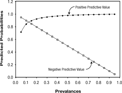
Figure 1: Effect of Prevalence on Positive and Negative Predictive Values

Table 14: Classification of Random Error

References

- Gordis L. Epidemiology. Philadelphia: W.B. 1996 Saunders Company. [Google Scholar]
- Rosner B. Fundamentals of Biostatistics. 1990 Boston: PWS-Kent Publishing Company. [Google Scholar]
- Conover W. J. Practical Nonparametric Statistics. 1971 New York: John Wiley & Sons, Inc. [Google Scholar]
- MacMahon B., Pugh T. F. Epidemiology: Principles and Methods. 1970 Boston: Little, Brown. [Google Scholar]
- Hennekens C. H., Buring J. E. Epidemiology in Medicine. Mayrent SL (ed) 1987 Boston: Little, Brown and Company. [Google Scholar]
- Glantz S. A. Primer of Biostatistics, 5th Edition. 2002 Ohio: McGraw-Hill Appleton & Lange. [Google Scholar]
- St Leger A. S., Cochrane A. L., Moore F. Factors associated with cardiac mortality in developed countries with particular reference to the consumption of wine. Lancet. 1979;1(8124):1017–1020. doi: 10.1016/s0140-6736(79)92765-x. [DOI] [PubMed] [Google Scholar]
- Kwon H. J., Cote T. R., Cuffe M. S., Kramer J. M., Braun M. M. Case reports of heart failure after therapy with a tumor necrosis factor antagonist. Ann Intern Med. 2003;138(10):807–811. doi: 10.7326/0003-4819-138-10-200305200-00008. [DOI] [PubMed] [Google Scholar]
- Ford E. S., Giles W. H., Dietz W. H. Prevalence of the metabolic syndrome among US adults: findings from the third National Health and Nutrition Examination Survey. JAMA. 2002;287(3):356–359. doi: 10.1001/jama.287.3.356. [DOI] [PubMed] [Google Scholar]
- Bazzano L. A., He J., Muntner P., Vupputuri S., Whelton P. K. Relationship between cigarette smoking and novel risk factors for cardiovascular disease in the United States. Ann Intern Med. 2003;138(11):891–897. doi: 10.7326/0003-4819-138-11-200306030-00010. [DOI] [PubMed] [Google Scholar]
- Vupputuri S., Batuman V., Muntner P. Effect of blood pressure on early decline in kidnery function among hypertensive men. Hypertension. 2003;42(6):1144–1149. doi: 10.1161/01.HYP.0000101695.56635.31. [DOI] [PubMed] [Google Scholar]
- Kannel W. B., Dawber T. R., Kagan A., Revotskie N., Stokes J., 3rd Factors of risk in the development of coronary heart disease - six year follow-up experience. The Framingham Study. Ann Intern Med. 1961;55:33–50. doi: 10.7326/0003-4819-55-1-33. [DOI] [PubMed] [Google Scholar]
- Vasan R. S., Larson M. G., Leip E. P. Assessment of frequency of progression to hypertension in non-hypertensive participants in the Framingham Heart Study: a cohort study. Lancet. 2001;358(9294):1682–1686. doi: 10.1016/S0140-6736(01)06710-1. [DOI] [PubMed] [Google Scholar]
- O'Donnell C. J., Larson M. G., Feng D. Genetic and environmental contributions to platelet aggregation: the Framingham Heart study. Circulation. 2001;103(25):3051–3056. doi: 10.1161/01.cir.103.25.3051. [DOI] [PubMed] [Google Scholar]
- D'Agostino R. B., Russell M. W., Huse D. M. Primary and subsequent coronary risk appraisal: New results from the Framingham study. Am Heart J. 2000;139(2 Part 1):272–281. doi: 10.1067/mhj.2000.96469. [DOI] [PubMed] [Google Scholar]
- The Atherosclerosis Risk in Communities (ARIC) Study: design and objectives. The ARIC Investigators. Am J Epidemiol. 1989;129(4):687–702. [PubMed] [Google Scholar]
- Harjai K. J., Boulos L. M., Smart F. W. Effects of caregiver specialty on cost and clinical outcomes following hospitalization for heart failure. Am J Cardiol. 1998;82(1):82–85. doi: 10.1016/s0002-9149(98)00234-3. [DOI] [PubMed] [Google Scholar]
- Strandberg T. E., Pitkala K., Berglind S. Multifactorial cardiovascular disease prevention in patients aged 75 years and older: a randomized controlled trial: Drugs and Evidence Based Medicine in the Elderly (DEBATE) Study. Am Heart J. 2001;142(6):945–951. doi: 10.1067/mhj.2001.119609. [DOI] [PubMed] [Google Scholar]
- Portney L. G., Watkins M. P. Foundations of Clinical Research Applications to Practice. 2nd edition. 2000 Upper Saddle River, NJ: Prentice-Hall Health. [Google Scholar]
- Mehra M. R., Ventura H. O., Chambers R. B., Ramireddy K., Smart F. W., Stapleton D. D. The prognostic impact of immunosuppression and cellular rejection on cardiac allograft vasculopathy: time for a reappraisal. J Heart Lung Transplant. 1997;16(7):743–757. [PubMed] [Google Scholar]
- Mandavia D. P., Hoffner R. J., Mahaney K., Henderson S. O. Bedside echocardiography by emergency physicians. Ann Emerg Med. 2001;38(4):377–382. doi: 10.1067/mem.2001.118224. [DOI] [PubMed] [Google Scholar]
- Katz D. L. Clinical Epidemiology and Evidence-Based Medicine: Fundamental Principles of Clinical Reasoning and Research. 2001 Thousand Oaks, CA: Sage Publications, Inc. [Google Scholar]
- Chen L., Chen M. H., Larson M. G., Evans J., Benjamin E. J., Levy D. Risk factors for syncope in a community-based sample (the Framingham Heart study) Am J Cardiol. 2000;85(10):1189–1193. doi: 10.1016/s0002-9149(00)00726-8. [DOI] [PubMed] [Google Scholar]
- Kim K. S., Owen W. L., Williams D., Adams-Campbell L. L. A Comparison between BMI and conicity index on predicting coronary heart disease: the Framingham Heart Study. Ann Epidemiol. 2000;10(7):424–431. doi: 10.1016/s1047-2797(00)00065-x. [DOI] [PubMed] [Google Scholar]
- Chambers R. B., Krousel-Wood M. A., Re R. N. Combined quality improvement ratio: a method for a more robust evaluation of changes in screening rates. Jt Comm J Qual Improv. 2001;27(2):101–106. doi: 10.1016/s1070-3241(01)27010-2. [DOI] [PubMed] [Google Scholar]
- Krousel-Wood M. A., Chambers R. B., Re R. N., Nitzkin P. R., Cortez L. M. Application of the combined quality improvement ratio in the evaluation of a quality improvement activity in a managed care organization. Am J Med Quality. 2003;18:117–121. doi: 10.1177/106286060301800305. [DOI] [PubMed] [Google Scholar]
- The beta-blocker evaluation of survival trial investigators: a trial of the beta-blocker bucindolol in patients with advanced chronic heart failure. N Engl J Med. 2001;344(22):1659–1667. doi: 10.1056/NEJM200105313442202. [DOI] [PubMed] [Google Scholar]