Cytopede: A Three-Dimensional Tool for Modeling Cell Motility on a Flat Surface

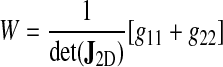
Abstract

When cultured on flat surfaces, fibroblasts and many other cells spread to form thin lamellar sheets. Motion then occurs by extension of the sheet at the leading edge and retraction at the trailing edge. Comprehensive quantitative models of these phenomena have so far been lacking and to address this need, we have designed a three-dimensional code called Cytopede specialized for the simulation of the mechanical and signaling behavior of plated cells. Under assumptions by which the cytosol and the cytoskeleton are treated from a continuum mechanical perspective, Cytopede uses the finite element method to solve mass and momentum equations for each phase, and thus determine the time evolution of cellular models. We present the physical concepts that underlie Cytopede together with the algorithms used for their implementation. We then validate the approach by a computation of the spread of a viscous sessile droplet. Finally, to exemplify how Cytopede enables the testing of ideas about cell mechanics, we simulate a simple fibroblast model. We show how Cytopede allows computation, not only of basic characteristics of shape and velocity, but also of maps of cell thickness, cytoskeletal density, cytoskeletal flow, and substratum tractions that are readily compared with experimental data.

1. Introduction

Animal cells plated on a flat culture dish, as is the case in the vast majority of laboratory experiments, take on an archetypal “fried egg” appearance. During migration, they spontaneously assume a polarized shape that varies according to cell type (e.g., hand-mirror for fibroblasts, or crescent for fish keratocytes). A thin sheet of cytoplasm extends at the leading edge (the lamellipodium) and undergoes cycles of protrusion, adhesion, and traction. Most of the time, this morphology is robustly preserved under perturbations but occasionally, certain maneuvers have drastic effects, in particular those that directly affect cytoskeletal organization.

The experimental methods of molecular and cell biology (imaging, biochemistry, genetics) have revealed a large number of the key chemical players and pathways involved in generating and controlling cell motility (Bakal et al., 2007; Jaffe and Hall, 2005). This information has been supplemented by biophysical approaches that include speckle imaging, FRAP, FLAP, atomic force microscopy and traction microscopy (Harris et al., 1980; Dembo et al., 1996; Dembo and Wang, 1999; Zicha et al., 2003; Waterman-Storer and Danuser, 2002; Danuser and Waterman-Storer, 2006). Unfortunately, analysis and integration of the massive datasets generated by these methods presents major conceptual, mathematical and numerical difficulties. To help bridge the gap we offer here a prototypical tool for cytomechanical modeling and computation, which we have named Cytopede. Cytopede is based on and extends an earlier computational environment for cytomechanics—the RIF, or “reactive interpenetrative flow” method (Dembo and Harlow, 1986).

The overarching scheme of Cytopede is derived from a sense that the issues and challenges involved in understanding cell motility are numerous and difficult but also highly modular and separable. Therefore, Cytopede starts by a process of deconstruction and analysis to enumerate and computationally implement fundamental physical components such as “viscosity” or “protrusive force” that drive a cell from one mechanical state to the next. These building blocks can then be combined and modulated in an infinite variety of ways.

In addition, Cytopede was designed to incorporate two key sets of attributes: first to automatically enforce fundamental laws of mass and momentum transport and conservation which, like everything else, cells must obey; second to allow straightforward contact with laboratory experiments. For the latter, compatibility with certain types of datasets is especially important. These are: (i) cell geometry which is simply given by the cell contour, and which may occasionally be complemented by information on cell thickness within that contour, (ii) cytoskeletal concentration, composition, reactivity and flow as revealed by fluorescent markers, and (iii) traction forces which can be determined via the deformable substratum method.

Cytopede is a software package dedicated to the simulation of free-boundary multiphase low-Reynolds number three-dimensional films in general and to the simulation of spread cells in particular. It uses the finite element method, distinguishes cytosolic from cytoskeletal dynamics (hence the label multiphase), and allows a wide range of shape changes as long as the ventral side of the cell that is modeled remains in contact with a flat substratum. Computationally innovative aspects include a new kind of adaptive mesh with specialized volume elements, surface elements, and line elements to allow for flexible implementation of free boundaries dynamics and of adhesion and detachment dynamics between a cell and its substrate.

As it matures, Cytopede is intended to be freely available to the community at large of researchers interested in modeling cell motility. The main objectives of this article are thus to some extent pedagogical and encompass the following themes: a discussion of the physical concepts that inform the approach used in Cytopede to address problems of cell motility; a description of the implementation of these concepts through the algorithms used by Cytopede; testing of the code through a numerical experiment performed on a viscous drop with surface tension spreading under the influence of gravity; and a biological example in which Cytopede is used to formulate and solve a simple model of a locomoting cell.

2. Physical Concepts

Compared to other instances of locomotion, the most remarkable feature of a migrating cell is the rapid chemical turnover of its structural elements. Cytoskeletal polymers are assembled at the front of the cell from components floating in the cytosol (actin monomers, cross-linkers, adhesion proteins, motor proteins, etc.). They are then disassembled, reassembled, and so forth through some unknown number of cycles, before reaching the rear. The simple fact that the reactivity of the cytoskeleton occurs on the same time scale as its motion means that the two phenomena cannot be separated and that a cell truly “makes itself anew” as it moves forward. Indeed, the importance and close connection between the chemistry and physics of the cytoskeleton has long been recognized in biophysical and modeling circles and has received overwhelming experimental confirmation (Watanabe and Mitchison, 2002). For the purposes of a physical analysis, the first consequence of this extreme reactivity is that it precludes models in which the cytoplasm is reduced to a single continuum. At minimum, it is necessary to consider interpenetrating cytosolic and cytoskeletal phases, and one must focus on the structural rules that govern the definition of the phases and the dynamical rules that govern their interconversion. Thus, actin monomers will contribute to the cytoskeletal phase if they are in the filamentous form and to the cytosolic phase when in the globular diffusible form but they cannot be part of both phases simultaneously.

With this in mind, consider the three principal structural components of animal cells:

• The cytoskeleton is a porous continuum consisting mainly of actin filaments that resists deformation through viscoelastic properties and is driven by molecular motors (e.g., myosin), polymerization forces, and thermodynamic (colloid) effects (e.g., electrostatic or steric).

• The cytosol flows passively through the cytoskeleton; it is a medium for the propagation of diffusible signals. It is incompressible and therefore conducts pressure. Finally, it can be converted to cytoskeleton via the polymerization of dissolved monomers (e.g., G-actin→ F-actin) and vice versa.

• The plasmalemma (or cortical membrane) defines the boundary of the cell by controlling (and often preventing) electrical, chemical and volumetric exchanges with the external medium. It is furthermore highly flexible to bending motions, highly fluid to shearing deformations, and yet very resistant to area expansions. Together, these three properties make it a good conductor of stress in the form of cortical tension.

Note that this classification ignores organelles, such as granules, or the cell nucleus. One could of course construct models that include such elements, but in most circumstances, the cost in terms of complexity becomes so large as to dominate the scientific return. In addition, the ability of cell fragments to migrate autonomously (Verkhovsky et al., 1999) lends further credibility to this approximation.

If one makes the key assumption that at the mesoscopic scale—i.e., at a scale small compared to the whole cell but large compared to individual molecules—the properties of the cell can be represented by continuous fields, then the general framework of continuum mechanics can be applied to animal cells just as it is done with any other materials. 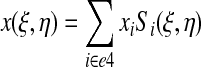Given a cell occupying a simply connected domain Ω(t) with boundary ∂Ω(t), Cytopede assembles an internally consistent set of coupled differential equations, boundary conditions and initial conditions that govern the temporal evolution of the domain itself and of various scalar and vector fields defined in its interior and on its surface. If is a position vector and t time, then the most basic and important fields are:

• θ_n(x, t) the network phase (cytoskeleton) volume fraction,

• θ_s(x, t) the solvent phase (cytosol) volume fraction,

• v_n(x, t) the network velocity field,

• v_s(x, t) the solvent velocity field, and

• P(x, t) the cytoplasmic pressure.

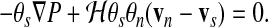
The evolution equations for the quantities θ_n, θ_s, v_n, v_s, and P are then determined by the laws of mass and momentum conservation.

Of note is that since it was developed in the context of cell motility in the 1980s (Dembo and Harlow, 1986), the two-phase fluid description is becoming more prevalent with several recent computational implementations (Rubinstein et al., 2005; Zajac et al., 2008).

2.1. Mass conservation

The fact that we only consider two phases (cytoskeleton and cytosol) mandates that the sum of network and solvent volume fractions is unity:

(1)

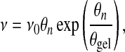
Net cytoplasmic volume flow is given by the sum of the flow of cytosolic volume and cytoskeletal volume, i.e. v = θ_nv_n + θ_sv_s. Since both components of the cytoplasm are condensed phases, it is an excellent approximation to regard the combined flow as incompressible (∇ · v = 0):

(2)

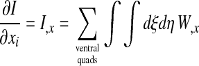
Finally, conservation of cytoskeleton implies that the rate of change of network concentration at a given point in space (Eulerian derivative) is the sum of an advective transport term describing the net inflow of network, and a source term which represents the net rate of in situ cytoskeletal production by polymerization:

(3)

Obviously depends on a prescription for local chemical activity that needs to be provided separately. Eq. 3 has a counterpart for the solvent

(4)

which, when taken together with Eq. 1 unsurprisingly reduces to Eq. 2. As a result, only Eqs. 1, 2, and 3 are needed and Eq. 4 is redundant.

2.2. Momentum conservation

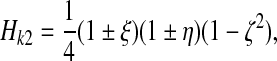
The momentum equations for the solvent and network phases are simplified by two observations. Because of the small dimensions and velocities involved, inertial terms can be neglected. Second, the essentially aqueous nature of the cytosol implies that its characteristic viscosity is not very different from that of water (0.02 poise). Since this is much less than typical cytoplasmic viscosities (∼1000 poise), the viscous stress is carried by the cytoskeletal (network) phase while the cytosolic (solvent) phase is nearly inviscid. Given these approximations, the only two forces that act on the solvent are pressure gradients and solvent-network drag—that is, the drag force due to solvent flow through the network when velocities are mismatched. In the spirit of Darcy's law, the solvent momentum equation can be written

(5)

P is the cytoplasmic pressure and it is assumed that, as for the partial pressures of a mixture of gases, it is shared by the cytosolic and cytoskeletal phases according to concentration (volume fraction). is the solvent-network drag coefficient more familiar as the product representing the hydraulic resistance that appears in the usual form of Darcy's equation. Theory (Scheidegger, 1960) as well as experiments on polymer networks (Tokita and Tanaka, 1991) give estimates of that lead to small drag forces compared to other forces acting within the cytoplasm, chief among them the cytoskeletal viscosity. This is not surprising since is roughly proportional to the solvent viscosity which is small compared to the network viscosity. The smallness of in turn implies that pressure gradients are small, or that pressure is close to uniform inside the cell; although, for a different view point, see Mitchison et al. (2008) and Charras et al. (2009). Thus, from the point of view of overall cell shape and motion as determined by cytoskeletal dynamics (Eq. 6 below), the precise value does not matter as long as it is sufficiently small. However, from the point of view of internal cytosolic flow, which can play an important transport role, the value of does matter, and pressure gradients, even though small are not negligible.

It is in the network (cytoskeleton) momentum equation that the rich complexity of cell mechanics becomes evident. Aside from pressure gradients and solvent-network drag, the network is also subject to viscous, elastic, and interaction forces, and the network momentum equation can therefore be written

(6)

Here, ν is the network viscosity, Ψ is the part of the network stress tensor remaining under static conditions, and F_ext is an external body force. The term Ψ can include inter-filament interactions (such as contractility due to myosin activity or swelling due to colloid osmotic effects), filament-membrane interactions, elastic forces due to deformations, etc.

2.3. Remarks on protrusive forces due to cytoskeleton-membrane interactions

Current ideas about cellular protrusion give a central role to the interaction of polymerizing filaments with the plasma membrane (Hill and Kirschner, 1982; Peskin et al., 1993; Dickinson and Purich, 2002; Kovar and Pollard, 2004). A comprehensive discussion of how such mechanisms can be described within a continuum mechanical framework is beyond the scope of this outline and will be the subject of a separate article, but we briefly mention key principles. As is always the case in the low Reynolds number regime, we require no net forces, so that any force on the membrane (e.g., for protrusion) must be balanced by an equal and opposite force on the network. This can be enforced automatically if the force is derived from the divergence of a tensor field Ψ^nM. In addition, because the membrane is fluid, cytoskeleton-membrane interactions cannot generate a shear stress in a patch of free membrane (this may change at adherent membrane). Then, at a patch of free membrane, the stress will be typically of the form:

(7)

where nn is the dyadic of the unit vector outward normal to the membrane and where ψ^nM is a scalar which may, for instance, be a function of local network density and/or polymerization at the membrane. In this work and elsewhere, we have essentially used a δ-function at the boundary which embodies the stress times its range d_M away from the membrane (Herant et al., 2003; Herant and Dembo, 2006) and set Ψ^nM = 0 elsewhere inside the cell. In a forthcoming work we will describe a more complete approach to the cytoskeleton-membrane interaction stress fields where the definition Ψ^nM at the boundary of the cell with condition Eq. 7 can be extended to define a more physical generalized membrane-network stress field in the intracellular space.

2.4. Boundary conditions

As partial differential equations, the evolution equations must be complemented by boundary conditions and this is where characteristics of the plasma membrane come into play. For mass conservation, we assume that the membrane remains impermeable to the cytoskeleton (which may even be anchored to the membrane) so that:

(8)

where v_M is the velocity of the boundary and n is the outward normal unit vector. If we also assume that the membrane is impermeable to the cytosol (which appears to be true in some cases and not in others) we also have

(9)

but this condition can be relaxed to allow a net volume flux through the boundary.

For momentum conservation, there are two main possibilities: (1) the boundary is constrained by interaction with a solid surface as in the case of the cell/substratum interface, or (2) the boundary is free membrane bathed by an inviscid external medium. In (1), the boundary condition reduces to a constraint on the normal component of the velocity (which must be 0), and, if a no slip condition also applies, there are additional constraints on tangential components of the velocity. In (2), the boundary condition amounts to a stress continuity requirement:

(10)

where γ is the surface tension, κ is the mean curvature of the membrane, n the outward normal to the membrane, and σ an externally imposed traction vector. This kind of boundary condition typically applies to the free back surface of the cell.

2.5. Constitutive equations

As presented, the mass and momentum conservation equations are cast in a general framework that must be defined by further prescriptions to provide closure of the system. Thus, the constitutive equations embody most of what one usually thinks of as the biological and regulatory aspects of cellular dynamics. These can be made complicated and detailed or simple and schematic depending on the specific modeling objective. As an example, it is plausible that the cytoskeletal viscosity ν (appearing in Eq. 6) should approach zero when the network volume fraction approaches zero. A simple scheme to satisfy this requirement would suggest that viscosity be determined by a constitutive law such as

(11)

prescribing a linear relation between viscosity and network concentration. A more complex idea designed to account for the possibility of network gelation may be expressed by

(12)

where θ_gel is a parameter that stipulates the volume fraction at which the probability of inter-filament crosslinking exceeds a percolation threshold for gelation. In principle, the form of the constitutive law for cytoskeletal viscosity could be verified empirically by investigating the rheology of the cytoplasm at various cytoskeletal concentrations; however, in general such experimental evidence is sparse and often difficult to interpret so that constitutive laws such as Eq. 12 are educated guesses.

The considerable uncertainties and complexities of physiological feedback and regulation make it likely that for the foreseeable future, progress in modeling cell motility will generally require a process of trial and error. It will be necessary to formulate various plausible constitutive relations, carry out computations to work out their consequences, and compare these consequences with experimental observations. It is in large measure to enable this process that we have created Cytopede, and it is also the reason why Cytopede is designed to allow maximum latitude for constitutive laws of every possible sort. Thus, the code allows the user freedom to set the constitutive laws that govern (the network formation or cytoskeletal polymerization rate), (the resistance to solvent flow through the network), Ψ (the network stress due to elasticity and static interactions), ν (the network viscosity), γ (the tension of the cortical membrane), along with other parameters that may govern behavior such as diffusion and transport of reactants, etc. In addition, it is also possible to define rules for attachment to and detachment from the substratum, processes that clearly play a key role in cell spreading and migration. The main advantage of this open and modular formalism is that one can start with a minimal and schematic approach and test the results and then gradually build complexity and detail step by step to virtually unlimited levels.

3. Computational Algorithms

Although we have tried to make it as self-contained as possible, this section presupposes a passing familiarity with the finite element method for which many textbooks exist; our favorite is Hughes (2000). In what follows, we outline the ideas behind Cytopede as well as key computational components. Algebraic developments are found in the Appendix. The Cytopede code itself is written in Fortran 90, and can be compiled and run on standard linux desktop PC workstations. For most of our visualization needs, we use gmv (General Mesh Viewer, freely available).

3.1. Numerical method and mesh structure

We use a Galerkin finite element method for several reasons. First, it is a well-established method for solving partial differential equation with solid theoretical underpinnings and with a considerable track record in many practical applications. We demand a conservative method that does not in itself add additional layers of uncertainty to computational results. Second, it is well-suited for free boundary problems and capable of accommodating the complex shapes and deformations observed in migrating cells. Third, it allows a straightforward and precise way of implementing the range of boundary conditions encountered in studies of cell motility despite a complex and dynamic boundary geometry.

For three-dimensional finite element simulations on an evolving computational domain, the management of the mesh represents the most arduous challenge, mainly because of the necessity to perform reliable automatic rezoning over a volume whose evolving shape cannot be predicted in advance. In addition, visualization and debugging difficulties increase exponentially with mesh complexity. This is why the overriding consideration in the selection of a mesh structure is for the maximum simplicity still compatible with a reasonably accurate simulation. This is also the reason why prior efforts to model spread cells have previously generally been limited to two-dimensional computations (Bottino et al., 2002; Rubinstein et al., 2005) or to semi-analytical calculations in the lubrication approximation (Oliver et al., 2005).

A spread cell on a substratum essentially represents a thin flat body. For this configuration, a pavement consisting of a single layer of 8-node brick elements is probably the simplest mesh structure possible but it has a drawback. In classic viscous film flow over a surface, the lower contact boundary has v = 0 while the upper free boundary has ∂v/∂z = 0, leading to a classic parabolic (Poiseuille) profile with height. The same probably holds true for certain cytoskeletal flows, in particular for centripetal flow where there may be anchoring at the substratum and retrograde flow higher up. For these types of flow, the linear resolution afforded by two nodes in height is inadequate. Instead we make use of a single layer of 12-node elements with quadrilateral ventral and dorsal faces and with 4 intermediate nodes located between the ventral and dorsal nodes (Fig. 1). This leads to quadratic accuracy vertically (sufficient to reproduce a Poiseuille type flow) and linear accuracy horizontally. However, horizontal resolution can be increased by mesh refinement while vertical resolution cannot.

FIG. 1.

An element in real (left) and natural (right) space. On the left, the nodes are labeled by stack and level.

We define as a stack a series of three nodes connected vertically. Thus each element is made up of four stacks, and in a given stack, the first node is the ventral node (usually with z = 0), the third node is the dorsal node, and the second node is the middle node. A stack is termed an edge stack if it lies at the edge of the mesh structure. The ventral nodes of edge stacks make up the contact line. The ventral surface of the domain consists of all the ventral faces of the elements. The back surface of the domain consists of all the dorsal faces of the elements together with the all the edge faces linking two edge stacks. Both these surfaces meet and are bounded by the contact line (Fig. 2).

FIG. 2.

A slice through a Cytopede simulation. Two elements are marked with those of their nodes that are visible. The internal element has a dorsal and ventral surface. The edge element has a dorsal and ventral quadrilateral surface, and an edge hexalateral surface.

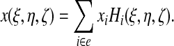
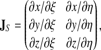
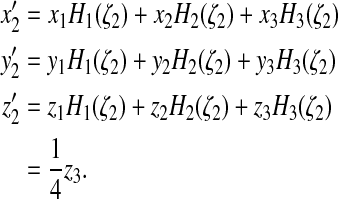
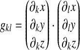
3.2. Shape functions

We use standard isoparametric shape functions corresponding to the mapping of an element from real coordinates (x, y, z) to natural coordinates (ξ, η, ζ; Fig. 1):

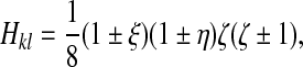(13)

for ventral (l = 1, ζ = −1) or dorsal (l = 3, ζ = + 1) nodes belonging to stack k where the signs are chosen such that the shape function is unity at node kl and vanishes at all others, and:

(14)

for middle nodes (l = 2, ζ = 0), and again the signs are chosen such that the shape function is unity at node k, 2 and vanishes at all other nodes of the element. Any field Φ defined at the nodes can be interpolated to an arbitrary position |ξ|, |η|, |ζ| ≤ 1 within an element as

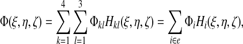(15)

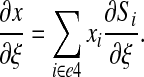
where i runs over all the nodes of a given element e. In particular, the mapping from natural coordinates to real coordinates is given by expressions of the type:

(16)

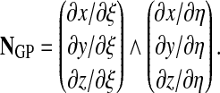
The Jacobian of the coordinate transformation is given by:

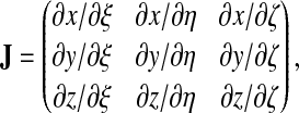(17)

with for instance

(18)

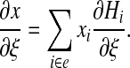
Partial derivatives of the field Φ can be computed, e.g.:

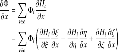(19)

where terms such as ∂ξ/∂x are computed by inverting the Jacobian J.

Surface shape functions S are defined in a way analogous to the volume shape function H. However, the form of an S depends on whether a quadrilateral (ventral or dorsal) or a hexalateral (edge) surface is considered. In the first case

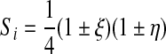(20)

where the signs are chosen such that the shape function is unity at node i and vanishes at the other 3 nodes that belong to the quadrilateral. In the second case,

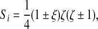(21)

if node i is a ventral or dorsal node and

(22)

if node i is a middle node. Signs are determined as before.

For a quadrilateral surface with natural coordinates ξ, η, the surface mapping from natural coordinates to real coordinates is then given by expressions of the type

(23)

where i runs over the 4 nodes of the quadrilateral e4. The Jacobian of the coordinate transformation (which is not square) is given by

(24)

with for instance

(25)

Similar expressions are obtained for edge surfaces by substituting ζ for η and running i over the 6 nodes of the hexalateral e6.

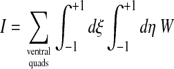
3.3. Quadratures

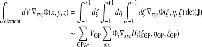
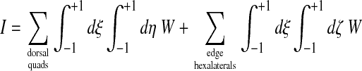
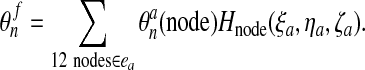
In our evaluation of volume integrals we use Gaussian quadrature with 12 Gauss points per element located at natural coordinates , , and :

(26)

where w_GP is the weight of the Gauss points (5/9 for and 8/9 for ζ = 0) and where det(J_GP) is the determinant of the Jacobian for the map xyz(ξ, η, ζ) evaluated at the Gauss points. The quantity

(27)

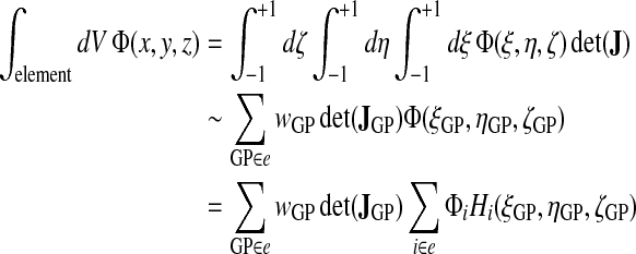
can be assimilated to the volume associated with a Gauss point, and the total volume of an element is therefore the sum of the volumes of its 12 Gauss points.

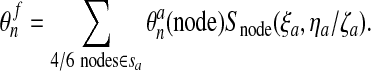
The evaluation of volume integrals of gradients is as follows:

(28)

where the real coordinate derivatives of the shape function H_i are evaluated at a Gauss point by inversion of the Jacobian J_GP (see Eqs. 17–19).

To compute surface integrals, we use 4 Gauss points for ventral or dorsal quadrilaterals, and 6 Gauss points for edge hexalaterals. The surface normal at a Gauss point is given (in the case of a quadrilateral) by

(29)

The area A_GP associated with a surface Gauss point is then given by

(30)

where w_GP = 1 for quadrilaterals. For hexalaterals, w_GP = 5/9 for the four Gauss points and w_GP = 8/9 for the two ζ = 0 Gauss points.

The integral of a surface field is then

(31)

where the index i runs over the four nodes of the quadrilateral e4 (or the hexalateral e6 with substitution of ζ_GP for η_GP).

The integral of the gradient of a scalar surface field can similarly be evaluated:

(32)

Details on how the surface gradient of a shape function (∇_SS_i) is computed are provided in the Appendix.

3.4. Basic computational sequence

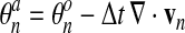
Given a network velocity field at time t, the simulation is advanced to t +Δt by means of five sequential operations:

• 1. Mesh Advection: An advected domain geometry is calculated by moving all mesh nodes with the local network velocity over the time interval Δt. If this motion causes a contact constraint to be violated (e.g., if the mesh motion causes a currently free surface to contact the substrate), then the contact line is advanced or retracted accordingly.

• 2. Rezoning: Nodes of the advected mesh are repositioned so that the distortion of volume and surface elements is minimized. The node movements during rezoning are constrained so as to preserve domain geometry (e.g., the contact line and the mesh surface contour and volume). The rezoning also maintains topology and number of elements.

• 3. Material Advection: The network, and all optional node attributes representing mass concentration of one kind or another are advected with the appropriate Lagrangian motion over the time interval Δt. The resulting fields are then interpolated to the new mesh generated by steps 1 and 2 (this approach is sometimes called a general Euler-Lagrangian advection scheme).

• 4. Diffusion and Reaction: All user-supplied constitutive rules controlling diffusion and reactions are evaluated for whatever chemical species may be included in the model. This usually involves determination of reaction rates, diffusion coefficients, and surface flux rates. Concentration of the various chemical species is then evolved on the new mesh over the interval Δt according to diffusive transport, chemical reactions and boundary fluxes.

• 5. Momentum Transport: All user-supplied constitutive rules controlling momentum transport are evaluated. This may involve the network viscosity, the surface tension of the plasma membrane, and many other parameters. The momentum equations, the incompressibility condition and applicable boundary conditions are solved to determine the pressure, network velocity and solvent velocity on the new mesh.

The above computational cycle is repeated until the desired termination condition is reached (i.e., a prespecified evolution time, or a prespecified behavior endpoint). Note that a simulation typically begins without an initial velocity solution, so that operation 5 must be performed first before entering the sequence 1–5.

The time step Δt is determined by the strongest of two constraints. First a Courant condition; given a velocity field the time step should not be more than 5% of the element crossing time. Second, a chemistry/diffusion constraint set by the monitoring of numerically estimated second time derivatives of the evolved species, and requiring 1% accuracy.

The overall approach is first-order accurate in time. We note that a higher order integration method would be an obstacle to the modularization of the individual tasks listed above that enables a relatively tractable computational process.

3.5. Step 1. Mesh advection

The basic requirement for the mesh is that its boundaries must follow the evolution of the boundaries of the cell, which is itself determined by the prior configuration and the cytoskeletal velocity field. For this reason it is desirable to have the mesh nodes move with the network velocity. However, without further intervention, such an approach would rapidly lead to severe distortion of the mesh with misshapen elements, and eventually, a computationally fatal folding of the mesh structure. Taking this into account, the mesh is evolved in a sequence of steps:

• 1. The mesh nodes move following the network flow, e.g., for node i

(33)

• where the superscript a designates the advected mesh, and the superscript o designates the old mesh.

• 2. The ventral node positions are readjusted vertically to have z = 0. This is necessary because ventral boundary conditions on the velocity are implemented with a penalty method that leads to very small, but nonzero vertical velocities (< 10⁻⁶ of the typical velocities in the problem). The readjustment to the z = 0 plane therefore has minimal impact on the calculation but makes life simpler.

• 3. The nodes of the contact line are shifted forward (and occasionally backward) if necessary. This is discussed in detail below, but the idea is that when the contact angle becomes >180°, the contact line advances. Similarly, it is possible to set a minimum contact angle below which the contact line retreats.

3.5.1. Forward motion of the contact line when the boundary condition is stick

When the velocity boundary condition at the substratum allows slippage, the contact line is simply advected with the matter as per Eq. 33. However when the velocity boundary condition at the substratum is no slip (v = 0), the situation demands more care. Our approach consists in letting the leading edge simply pivot down around the contact line and make contact with the substratum in a natural way. Note that this is only possible because the elements are quadratic in height.

Consider an edge boundary stack of three nodes 1, 2, and 3 (Fig. 3). The parametrized equation of the edge curve is given by:

(34)

FIG. 3.

Side view of the contact line. t is the leading edge tangent at the contact point, α is the contact angle (left), and n is the outward normal to the contact line. When the middle node 2 descends below one quarter of the height of the dorsal node 3, the contact angle become larger than 180°, and the leading edge effectively penetrates the substratum. Node 1 is then moved to position 1′, and node 2 is moved up along the leading edge to one quarter of the height of the dorsal node 3 so as to restore a contact angle of 180° exactly.

and similarly for y and z where the L's are one-dimensional shape functions: , and . Let t be the tangent to this edge curve. We have

(35)

and similarly for t_y and t_z. At the contact line (which coincides with node 1), we have ζ = −1, and z₁ = 0:

(36)

We now define n_CL, the outward normal to the contact line. The contact angle α is then given by:

(37)

It is clear that if t_z < 0 or equivalently , the contact angle is <0° (rare) or > 180° (common in spreading) and the contact line node needs to move.

The procedure is thus as follows (Fig. 3): if for an edge stack, we have this means that there exists ζ₁ > −1 such that z(ζ₁) = 0 (i.e., the edge curve crosses the substratum twice, once at ζ = −1 which corresponds to node 1, and once at ζ = ζ₁). We therefore displace node 1 to position 1′:

(38)

We also move 2 to 2′ at the position determined by ζ₂ such that :

(39)

This returns the contact angle to 180°.

3.6. Step 2. Rezoning

• 1. The nodes are repositioned to optimize the mesh configuration without changing the boundaries.

  • (a) The nodes on the contact line are rezoned to be equidistant from one another. The procedure is described in Figure 4.

  • (b) The dorsal edge and middle edge nodes are shifted along their tangent planes so as to lie in the plane perpendicular to the substrate z = 0 and containing the contact line normal. The displacement keeps the elevation of the edge nodes above the substratum (z) constant and prevents distortions of the edge of the mesh.

  • (c) The interior ventral nodes are rezoned to minimize the two-dimensional Winslow functional (see below).

  • (d) The dorsal nodes and middle edge nodes are rezoned to minimize the two-dimensional Winslow functional (see below).

  • (e) The interior middle nodes are rezoned to minimize the three-dimensional TTM functional (see below).

    The end-result of this sequence is a new rezoned mesh .

• 2. The nodes belonging to the back surface of the rezoned mesh are projected onto the surface of the advected mesh to obtain a “projected mesh” (for all other nodes, ).

• 3. The final new mesh is obtained by a linear combination of the rezoned mesh and projected mesh:

(40)

FIG. 4.

Accordion effect during rezoning. Left: top down view of three ventral contact line nodes labeled 1,2,3. Node 2 needs to move closer to node 3. Let m be the median between node 1 and 3, and t the volume tangent at node 2. A volume conserving rezone would move node 2 along t towards the intersection with m (solid arrow). A boundary rezone would be to move node 2 along the boundary line (23), but this is not volume conserving. In practice we use a weighted average of the two (90% volume rezone and 10% boundary rezone). The boundary rezone contribution is to avoid an accordion instability as described on the right, where tangent node motion to even out inter-nodal distances only worsens the situation.

The reason we do not use the rezoned mesh directly is to attempt to avoid the accordion effect described in Figure 4.

3.6.1. Rezoning of the ventral surface

Once the positions of the ventral edge nodes of the contact line have been set, the interior ventral nodes of the mesh (but not the edge ventral nodes which make up the contact line!) are rezoned to optimize the ventral mesh. Our general approach follows that described in Knupp and Steinberg (1993). It is variational in that the ventral nodes interior to the contact line are repositioned to minimize a functional integral I over the entire ventral surface:

(41)

where W is the Winslow functional, a local measure of two-dimensional mesh distortion:

(42)

where g_kl are the components of the Riemann metric tensor of the ventral surface;

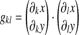(43)

and the indices k and l run over the natural surface coordinates ξ and η. The determinant of the two-dimensional surface Jacobian det(J_2D) (see Eq. A-3) essentially corresponds to an elementary surface area (see Eq. 30) so that the functional is dimensionless. Details on the computation of W and derivatives are provided in the Appendix.

We minimize I by Newton's method. Let

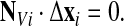
(44)

denote the derivative of I with respect to displacement δx of ventral node i. Note that in the sum, only the few quadrilaterals to which node i actually belongs make a nonzero contribution. An estimate of the displacements of Δx_i and Δy_i of node i that minimize I is given by the system

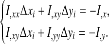(45)

In practice however, all the nodes are coupled so it is prudent to damp the motion while iterating to minimize I (we use a factor of 1/2 and further constrain the motion to 10% of the local element length scale).

3.6.2. Rezoning of the back surface

Rezoning of the back nodes follows the same principles as for the ventral surface. Once again, edge nodes that belong to the contact line are not moved, but there are some additional complexities from the fact that the surface is not planar and that we have to deal with dorsal quadrilaterals and edge hexalaterals. Thus, the functional integral I is now

(46)

where, as before, W is the Winslow functional defined in Eq. 42 and the components of the metric tensor are:

(47)

where the indices k and l run over the natural surface coordinates (ξ, η for dorsal quadrilaterals and ξ, ζ for edge hexalaterals).

Minimizing I by Newton's method with respect to the displacement of node i involves a 3 × 3 system:

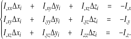(48)

This time however we need to add constraints. First the displacement of a node must be restricted to the plane tangent to the surface, or more precisely, to the plane along which node motion preserves volume. Let N_Vi be the normal to the volume tangent plane at a node i (see Appendix for the calculation of N_Vi, Eq. A-13), the rezoning of node i must be in that plane and so must satisfy

(49)

Second, to preserve the contact angle during the motion of the middle and dorsal edge nodes (here labeled 2 and 3) the displacement must satisfy:

(50)

These two constraints can be implemented via the method of Lagrange multipliers.

3.6.3. Rezoning of the interior nodes

Once all the surface nodes have been rezoned, the middle nodes belonging to interior stacks need to be repositioned. This is also accomplished via a variational principle on a functional:

(51)

where T is a three-dimensional extension of the Winslow functional generally known at the TTM functional Knupp and Steinberg (1993):

(52)

where the g_kl's are as before (Eq. 47) and the indices k and l run over the intrinsic coordinates ξ, η, and ζ, and det(J) is simply the determinant of the three-dimensional Jacobian (Eq. 17).

As for surface nodes, we compute the derivatives of I with respect to the motion of individual nodes and minimize I using Newton's method and solving the system given by Eq. 48 (the necessary derivatives of T are provided in the Appendix). There are no constraints on the displacement of interior nodes.

Here an attentive reader may ask why not simply use the TTM functional for all nodes with appropriate constraints for the boundary nodes? We have attempted this and found it to lead to poor mesh structure at the edge of the mesh, an obviously critical region in studies of thin films.

3.7. Step 3. Material advection

We use a Lagrangian-Eulerian method to update the network concentrations θ_n from t to t + Δt. First comes the Lagrangian step which corresponds to the advection of the mesh with the flow of network (Eq. 33):

(53)

where is the original network concentration at a given node, and is the network concentration at that same node after the node has been advected with the network velocity. If one considers a reference volume V^o around the original node and advects it with the network flow to V^a, then obviously

(54)

(which is the same as saying Δt∇·v_n = (V^o − V^a)/V^o). A given node belongs to several elements, and for each of these elements, it has a nearest Gauss point (each element has 12 nodes and 12 “matching” Gauss points). We choose as our reference volume the sum of the V_GP corresponding to the Gauss points associated with a node so that

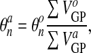(55)

where the volumes V_GP are computed for the original and advected mesh and through Eq. 27.

Second comes an Eulerian step which corresponds to the rezoning of the mesh from to . Here, the procedure is simply to interpolate from . Given an interior node in the final mesh, the element e_a of the advected mesh that contains it is determined along with the natural coordinates ξ_a, η_a, ζ_a of the node in e_a. We then have

(56)

For boundary nodes in the final mesh, the closest point on the surface of the advected mesh is determined with natural coordinates ξ_a, η_a or ξ_a, ζ_a as the case may be. We then have:

(57)

It is possible to advect chemical species in the solvent phase by using the same procedure as outlined above, except that the advected mesh is now the result of node motion according to the solvent flow field v_s. However, we have found that advection of chemical species in the solvent (cytosolic) phase is most often negligible compared to diffusion (i.e., the Peclet number is small) so that usually, the only important step is interpolation from the original to the final mesh.

3.8. Step 4. Diffusion and reaction

Diffusion-reaction problems are standard fare and we will limit ourselves to a brief outline of an implicit backward Euler scheme with finite element treatment of spatial derivatives and boundary conditions. For a chemical species c, we need to evolve

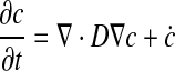(58)

between t and t +Δt, where D is the diffusion coefficient, and ċ is the rate at which the species is created by chemical reaction. We will assume that at time t, we know D, c^o, ċ^o, and ∂ċ^o/∂c (evaluated via appropriate constitutive laws when necessary). Discretizing in time, we can then write:

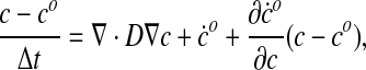(59)

where c is the species concentration at the end of the time step. Rearranging the terms we obtain

(60)

Following the canonical Galerkin finite element approach—which is beyond the scope of this work and is described in standard texts (Hughes, 2000)—Eq. 60 can be recast in a weak (variational) form while simultaneously expanding c over a set of trial functions (the shape functions). This leads to a linear system determining the vector c_i where i runs over the all the nodes (and corresponding shape functions):

(61)

where Q is a square “stiffness” matrix, and f is a “load” or “force” vector. Two nodes i and j belonging to the same element e contribute to the stiffness matrix and to the load vector via their associated shape functions H_i and H_j:

(62)

and

(63)

So that in the end Q_ij = Σ_eQ_ij,e and f_j = Σ_ef_j,e.

Dirichlet and Neumann boundary conditions lead to modifications of the diffusion equation Eq. 58 that look like:

(64)

where c_ext is an external reference concentration and Π is an effective permeability (the higher Π, the stricter the Dirichlet boundary condition c = c_ext), and where is a source term corresponding to a Neumann boundary condition. For a Dirichlet condition, both the stiffness matrix and the load vector must be modified:

(65)

(66)

To take into account an external chemical gradient, one can easily make c_ext a function of coordinates (e.g., to model chemotaxis).

For a Neumann condition, only the load vector changes

(67)

In practice, we solve Eq. 61 through the conjugate gradient method with preconditioning (simple diagonal matrix of (1/Q_ii)'s), although for problems with a small number of nodes, direct LU decomposition is feasible.

Two-dimensional surface diffusion is implemented in a similar manner except that elements are now quadrilaterals and hexalaterals, surface shape functions are used instead of volume shape functions, and boundary conditions apply to lines (e.g., the contact line) instead of surfaces.

3.9. Step 5. Momentum transport

Because of the multiphase nature of the flow (one has to solve the triplet v_n, v_s, and P rather than just for v and P) some modifications are required compared to the usual single phase viscous flow finite element treatment.

Recall the solvent and network momentum equations

(68)

and

(69)

By adding the solvent and network momentum equation together, v_s can be eliminated to obtain a “bulk” cytoplasmic momentum equation

(70)

which we call the “velocity equation.” The boundary conditions can be free or contact. For free membrane, stress continuity requires

(71)

where P_ext is the external pressure, γ and κ the surface tension and mean curvature, and σ is the boundary traction. For contact boundaries, Dirichlet conditions are imposed on the velocity.

The solvent momentum equation (Eq. 68) gives an expression for v_s:

(72)

which can then be substituted in the incompressibility condition to yield:

(73)

or, if we relabel

(74)

which we call the “pressure equation.” In situations where there is zero membrane permeability (i.e., no trans-membrane solvent flow), the boundary condition simplifies to:

(75)

The general strategy to obtain a solution follows Uzawa's algorithm: an initial guess for the pressure field (which is usually good since obtained from the previous time step) allows the computation of the network velocity field by Eq. 70. This velocity field can then be used to update the pressure field by Eq. 74, and so on through iterations between the two equations. Once the network velocity field v_n and pressure field P have converged to a self-consistent solution, the solvent velocity field v_s can be trivially extracted through the use of Eq. 72 with automatic enforcement of the incompressibility condition.

To solve the velocity equation (Eq. 70), we wish to compute the vector u which assembles the three velocity components of every node (i.e., u has 3N components where N is the number of nodes):

(76)

where K is a square stiffness matrix, and f is usually known as the “force” vector. Expressions for the contributions by individual elements to the stiffness matrix and the force vector can be derived from Eq. 70. If i and j are two nodes that belong to element e, they make the following contributions to the stiffness matrix:

(77)

(78)

and to the load vector

(79)

where the last term really amounts to , where V_e is the volume of the element. In the end, the components of K and u are given by K_ixjx = Σ_eK_ixjx,e and f_jx = Σ_ef_jx,e.

Once new nodal network velocities have been estimated for a given guess of the pressure field P^o (obtained from the previous cycle of iteration between velocity and pressure equations, or from the prior time step if this is the first pass), we solve the pressure equation (Eq. 74) to obtain a new pressure field P. Unfortunately, direct solution of Eq. 74 leads to severe instabilities so that the following damped evolution equation is solved instead:

(80)

where r > 0 is a relaxation coefficient. Note that since, within a given time step, we iterate back and forth between the velocity and pressure equations until the velocity and pressure fields have converged to a stable value, the LHS of Eq. 80 tends to 0 (P and P^o will be the same) as we get closer to the solution so that in the final analysis, it is Eq. 74 that is solved. The relaxation coefficient is taken to be proportional to the perturbation of the velocity field by a perturbation in pressure:

(81)

In the code, r is evaluated numerically using the velocity equation (Eq. 70) and β is set to 10² for small Φ (typical cytoplasmic condition) and 10³ for large Φ (single phase viscous flow condition). We can rewrite Eq. 80 as:

(82)

which is to be cast by the finite element approach into a linear system of equations

(83)

where Q is a square stiffness matrix, P is the vector of nodal pressures that we seek, and g is a load vector. Individual element contributions from element e to Q and g are given:

(84)

and

(85)

so that Q_ij = Σ_eQ_ij,e and g_j = Σ_eg_j,e.

Boundary conditions to these equations can take a multiplicity of forms that cannot all be covered here. The most important cases are the contact velocity boundary conditions on the ventral surface (substratum), and the contribution of the surface tension to free boundary dynamics.

For instance, if the x component of v_n must be constrained at a surface containing node i, as would be the case for a ventral quadrilateral with a no-slip velocity boundary condition at the substratum, we add a diagonal term to the velocity equation stiffness matrix;

(86)

where is a “penalty” viscosity set many orders of magnitude greater than the average problem viscosity . If a viscous drag between network and substrate is desired instead of a no-slip condition this is easily implemented by the use of an appropriate viscosity coefficient.

The load on a given surface node due to the surface tension γ is −∇_i(γA), where A is the surface area and where the gradient is taken with respect to motion of node i. We therefore add a term to the velocity equation vector load:

(87)

Details on how to compute this gradient are given in the Appendix.

In practice, we solve both equations through the conjugate gradient method with preconditioning (for the pressure equation with the diagonal matrix (1/Q_ii), for the velocity equation with the block diagonal matrix obtained by local inversions of the 3 × 3 nodal stiffness matrices . Convergence is judged to be sufficient for relative changes <10⁻⁴ in pressure and velocities. For an ongoing simulation where the initial guess is close to the solution, this typically occurs within 10–20 iterations, but for a new problem, it may take several hundred iterations. Even when convergence is rapid, solving the momentum equations is almost always the most computationally intensive part of the simulation.

4. Testing: The Sessile Drop

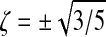
Consider a hemispheric drop with radius and height a₀ = h₀ = 1, viscosity ν = 10³, and surface tension γ = 1 sitting in equilibrium on a non-wetting surface with no-slip boundary condition (v = 0). At time t = 0, “gravity” is turned on in the form of an external body force F_z = −10² so that the Bond number becomes large: . The drop flattens, and after the contact angle becomes 180° (the substratum is non-wetting), the contact line begins to advance. Eventually, the gravitational work gained by further flattening is balanced by the surface tension work of area expansion, and the sessile drop settles in a new equilibrium shape, still with contact angle 180°. Note that we do not give units—the reader is free to assume cgs or SI or any other self-consistent units.

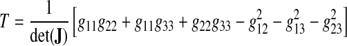
We have chosen this problem as a benchmark for several reasons. First it is simply posed and simply explained. Second, it has received attention for more than a century (Bashforth and Adams, 1883), and although it cannot be solved analytically, several useful approximations are available. Third, because of the large Bond number, it leads to a very flat drop with an aspect ratio ∼ 20: this is representative of our intended application of Cytopede to model flattened cells as thin films. Fourth, it has cylindrical symmetry which allows comparisons with reference two-dimensional numerical simulations performed with another finite element code that has been previously validated (Dembo, 1994; Drury and Dembo, 1999).

This single phase flow application requires phase locking between the solvent and the network, which can be achieved by setting a large network-solvent hydraulic resistance (see Eq. 68). We use

(88)

where L is the local length scale of an element which we have found to be a safe choice, large enough so that network-solvent slippage is insignificant, but not so big so as to lead to the spurious pressure modes that appear in finite element calculations when the Babuska-Brezzi condition is violated (Drury and Dembo, 1999).

The results of the simulations are presented in Table 1 and in Figures 5–7. It is apparent that both two- and three-dimensional calculations have converged numerically. For the two-dimensional calculations, a low resolution simulation with 641 nodes (562 elements) gives essentially the same result as a high resolution simulation with 2405 nodes (2248 elements). For the three-dimensional calculations, a simulation with 1035 nodes (308 elements) gives essentially the same result as a simulation with 3051 nodes (944 elements).

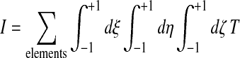
Table 1.

The Spreading Drop: Theory versus Numerical Experiments

	Theory	2D calculation	3D calculation
V0	2.094	2.085	2.084
V∞	2.094	2.078	2.128
h∞	0.2	0.203	0.205
a∞	1.83	1.82	1.86

V, h, and a are, respectively, the drop volume, maximum height, and average radius of the contact line. For the numerical simulations, t = 10,000 was taken as t_∞. Simulation results in 2D and 3D correspond to the high-resolution calculations.

FIG. 5.

Meshes for two- and three-dimensional high-resolution simulations at time t = 0 and t = 2000. Note that in the two-dimensional simulation the actual mesh used in the computation is half of what is shown. Note also the three-dimensional mesh consists of a dorsal layer (shown), a ventral layer, and an intermediate layer (not shown).

FIG. 7.

Profile of the surface of the drop. Points correspond to the three-dimensional high-resolution simulation at t = 100. Solid lines correspond to the two-dimensional high-resolution simulation at t = 100 and t = 165.

The equilibrium state (t → ∞ in the present set up) has been studied extensively and expression for the ultimate height and radius derived: h_∞ = 2(γ/F_z)^1/2 = 0.2; (although there can be a potential correction factor <5% as is noted in Padday and Pitt (1972), and (Rienstra, 1990) so that a_∞ = 1.83. The three-dimensional (and two-dimensional) simulations converge asymptotically to similar limits, with a very slightly larger drop size in the 3D simulation which is in part due to a small upward drift in volume (∼2%) over ∼5000 time steps of the calculation (Table 1).

Looking at the dynamic evolution from the initial configuration toward the equilibrium state, analytic guidance is unfortunately restricted to an investigation of the dynamic motion of the contact line before reaching equilibrium which gives as an approximation (Hocking, 1983); this is close to our calculations. For further insights, we are therefore limited to a comparison between the two-dimensional and three-dimensional simulations. In both the two-dimensional and three-dimensional calculations, the contact line radius a initially equal to a₀ = 1 begins to change at t ∼ 18; this is the time it takes for the contact angle to increase from 90° at t = 0 to 180°. There is however an early deviation between the time-dependence of the height and contact line radius as computed by the two-dimensional and three-dimensional codes. Close inspection reveals that, in the early evolution, the height of the drop decreases much faster in the three-dimensional calculation than in the two-dimensional calculation (Fig. 6). This inaccurate velocity solution in the three-dimensional calculation is due to limited vertical resolution using only 3 node (one element) interpolation—we are here far from the thin film regime with an initial aspect ratio of only 2. Because mass initially flows faster from the top to the sides of the drop, the radius of the contact line a takes an early lead in the three-dimensional compared to the two-dimensional calculation. As the drop thins, the three-dimensional calculation becomes more accurate, but the shift in the contact line evolution subsists. For instance, the drop profile obtained at t = 100 with a three-dimensional simulation is significantly different from that obtained with the two-dimensional calculation at the same time, but exactly matches the two-dimensional solution at t = 160 (Fig. 7). Improvements to the early part of the three-dimensional calculation would require additional layers of elements. However, in most conditions that pertain to cells on a substratum, aspect ratios are large and the three-dimensional code should perform adequately.

FIG. 6.

Evolution of the contact line radius a (top) and the drop height h (bottom) with time. Doted lines represent theoretical estimates, a_∞ = 1.83, a ∝ a⁷ and h_∞ = 0.2 (see text). Dashed lines represent output from the low- and high-resolution three-dimensional simulations. Solid lines represent output from the low- and high-resolution two-dimensional simulations (indistinguishable for h). The step-like nature of the a curve for two-dimensional simulations comes from the fact that the contact line advances by a discrete jump when a new element comes into contact with the substratum.

5. Application: A Model of the Fibroblast

We now turn to the intended purpose of Cytopede—the simulation of locomoting cells, and present a basic cytomechanical model consisting in a set of rules (constitutive relations and boundary conditions) that leads to fibroblast-like behavior. This example is then used to show how contact with quantitative experimental observations may be achieved. Note that rather than striving for verisimilitude, we have attempted to develop a pedagogical and informative scenario. Nevertheless, while this model represents a gross simplification of what must be a very complicated collection of physico-chemical processes in a real cell, it still represents a large increase in complexity over the simple spreading drop.

5.1. The model

The key parameters used in the model are listed in Table 2 and fall into two broad categories: diffusion-reaction parameters that determine in space and time the biochemistry of the cytoskeleton, and mechanical parameters that determine the dynamical behavior of the cytoskeleton. Choices for many of these parameters were inspired from previous two-dimensional models of neutrophils (Herant et al., 2003, 2005, 2006).

Table 2.

Parameters Used for the Model Fibroblast

Parameters	Symbol	Value
Cytoplasmic volume	Vc	1080 μm3
Biochemical parameters
Baseline network density	θ0	10−3
Network turnover time	τn	20 s
Messenger concentration	m	—
Equilibrium network	θeq = θ0(1 + m)	—
Messenger diffusion coefficient	Dm	1 μm2 s−1
Messenger decay time	τm	1 s
Messenger penetration depth		1 μm
Messenger emissivitya	εm	0–20 μm s−1
Mechanical parameters
Specific network viscosityb	ν0	1 × 105 Pa s
Disjoining force strengthc		(10 × mθn) mN m−1
Flattening force strengthc		(−400 × εm) mN m−1
Network-solvent drag		100 pN s μm−4
Slip contact angle	αs	60°
Surface Tension	γ0 (A/A0)3	0.01 (A/A0)3mN m−1

^aUnits are length/time instead of 1/(area time) because m is dimensionless instead of 1/volume.

^bBaseline viscosity is thus θ₀ν₀ = 100 Pa s.

^cThe dynamically relevant term is the network-membrane potential energy times its range d_M or d_s.

5.1.1. Biochemical parameters

The baseline volume fraction of network θ_n is set to θ₀ = 10⁻³, but must increase several fold near the leading edge (up to θ_n ∼ 2 × 10⁻²). To achieve this, we set (see Eq. 3)

(89)

where θ_eq is the local equilibrium network concentration, τ_n = 20 s is a network turnover or equilibration timescale modulated by the local (dimensionless) concentration m of a polymerization messenger:

(90)

The polymerization messenger species is generated at activated portions of the plasma membrane and diffuses into the cytoplasm with diffusion coefficient D_m = 10⁻⁸ cm² s⁻¹ and lifetime τ_m = 1 s:

(91)

where we neglect advection by the local flow (the Peclet number is small). The Neumann boundary condition at the membrane is

(92)

where is the local emissivity of the messenger. In the simulations, is set to be maximum near activated portions of the contact line and zero further in, so that m ∼ 20 near the leading edge, and rapidly decays into the cytoplasm over the penetration depth d_m = (D_mτ_m)^1/2 = 1 μm.

The messenger is of course just a way to encode positional information as a driver of cytoskeletal chemistry and activity. In the real cell, a host of biochemical intermediates perform this task, and so, this simple “messenger” is not intended to represent any single molecule.

5.1.2. Mechanical parameters

We assume that the viscosity of the cytoskeleton is proportional to its density so that in the momentum equation (Eq. 6):

(93)

with ν₀ = 10⁵ Pa s, so that the baseline viscosity is ν₀θ₀ = 100 Pa s, and reaching maximal values of 1000 Pa s at the leading edge.

To drive protrusion, we implement a network-membrane repulsive stress term which has the form:

(94)

where nn is the dyadic of the unit vector outward normal to the membrane. For , a normal stress pushes the membrane outward and the network experiences an equal an opposite reaction driving it inward, so that this stress corresponds to a disjoining force that expands the cortical network layer. In a polymerization force model such as is used here, there is a linear dependence on the local polymerization rate (driven by the messenger concentration m) and the network density θ_n. Note that is set to zero at the ventral surface of the cell because the network is assumed to be anchored to the substratum.

The actual relevant dynamical parameter is the stress times its range d_M away from the membrane (this is a somewhat subtle point; see discussions in Herant et al., 2003; Herant and Dembo, 2006). With , the messenger concentration at the leading edge m ∼ 20, and taking d_M = 1 μm, the stress energy within the layer is ∼ 1.8 k_BT per actin monomer. The physical origin of this stress is left unspecified but may involve buckling of filaments against the membrane (Kovar and Pollard, 2004), long-range electrostatic interactions, or entropic constraints, which transform the chemical energy of polymerization into a stress capable of producing mechanical work.

To prevent the protrusive stress from bulging the membrane upward rather than forward, it is necessary to postulate a compensatory force directed down toward the substratum, or else to assume a planar geometry of the cytoskeleton that only allows growth in the horizontal direction (so that most of the z terms in the stress-tensor vanish), something we find implausible. We therefore implement a network-substratum attractive stress term which has the form

(95)

where nn is the dyadic of the unit vector downward normal to the substratum. For , the stress pulls the network down towards the substratum. Again the dynamically relevant quantity is the stress times its range d_s (Herant and Dembo, 2006). With at the leading edge (), and assuming d_s = 1 μm, this leads to a maximum downward force at the leading edge of 800 pN per μm² of ventral membrane. Again, the physical origin of this force is left unspecified, but may involve molecular motors such as unconventional myosins which are often detected at the leading edge of locomoting cells (Fukui et al., 1989; Yonemura and Pollard, 1992; Wagner et al., 1992; Sousa and Cheney, 2005).

We finally note that aside from the flattening force described above, this model of the fibroblast does not include contractile elements of the kind that might represent the activity of myosin II bundles often detected in the cell body. Such components could readily be incorporated but for the sake of simplicity, we do not do so here.

5.1.3. Boundary conditions

We assume impermeability of the plasma membrane to both cytosol and cytoskeleton (Eqs. 8, 9) so that total volume is conserved. For the ventral interface in contact with the substratum, the boundary condition on the network velocity is no slip (v_n = 0): we postulate that adhesion via transmembrane proteins locally immobilizes the cytoskeleton rigidly (for simplicity, viscous slippage is not considered but could be implemented easily to match behaviors of the type described by Leibler and Huse 1993). Thus, when new membrane at the leading edge comes into contact with the substratum we assume immediate adhesion. The only exception is the trailing edge of the cell where we allow movement when the contact angle decreases to less than 60°.

For the back surface of the cell, the motion of the free boundary is determined per Eq. 10 with the surface tension

(96)

where A is the total surface area of the cell, A₀ is the area of a volume-equivalent sphere (a constant since volume is conserved), and γ₀ = 0.01 mN m⁻¹ is a baseline surface tension. We have found that the exact form does not matter as long as the tension rises steeply with area; what counts is that the tension become sufficiently strong to limit cell spreading to a plausible extension. In the simulations, once the cell is spread, A/A₀ ∼ 2–3 so that γ ∼ 0.1–0.4 mN m⁻¹.

5.2. The simulation

The initial condition is that of a hemispherical cell with cytoplasmic volume V_c = 1080 μm³ (a reasonable estimate of fibroblastic volume without nucleus (Uhal et al., 1998). The entire cell circumference is activated so that protrusion due to network polymerization drives the contact line out. As the cell flattens (Fig. 8), the surface area increases and so does surface tension (Eq. 96) thus resisting further extension. After ∼ 100 s, the cell takes on a stable disk shape with diameter of ∼33 μm, and height of ∼1.5 μm. The surface tension at which protrusion stalls is ∼ 0.34 mN m⁻¹ and can be readily identified with a force of protrusion of ∼700 pN per μm of leading edge (the doubling is due to the fact that both dorsal and ventral folds of membrane are pulling back).

FIG. 8.

Time series of evolution of a fibroblast model. Hemispherical cell (t = −100 s) flattened to an equilibrium disc shape (t = 0 s) by activation of the entire contact line. After 85% of the contact line is rendered inactive, an elongated fibroblast like shape emerges (t = 20, 100, 300, 600 s).

From this equilibrium disk shape, we break the symmetry by abrogating contact line activation over 85% of the circumference. Messenger production and therefore network polymerization continues over the remaining 15% of the contact line. Note that as the overall perimeter length of the cell changes because of deformation of the contact line, activation is maintained over 15% of that length. In addition, when the contact angle becomes <60°, we force a return of the contact angle to 60^∘ by shifting the contact line which enables retraction of the trailing edge.

As a result of these changes, a leading edge stretches out ahead while the remainder of the perimeter slowly retracts and forms a tail (Fig. 8). Eventually, a longitudinally elongated, approximately triangular cell emerges with length of ∼40 μm and leading edge migration velocity of order 0.06 μm s⁻¹.

Because the shape of the model fibroblast is not stable, distortion eventually grows beyond the abilities of the rezoning algorithm to maintain an adequate mesh. For this particular model, this occurs at t = 600 s, by which time the code has taken ∼7,000 time steps. The calculation takes approximately 3 hours on a PC workstation (running on a single CPU).

5.3. Contact with experimental data sets

Four principal aspects of the mechanical characteristics of cells are experimentally accessible and available in the general literature.

• 1. The basic contour and motion of the cell,

• 2. The thickness h of the cell as a function of position x, y and time t,

• 3. The cytoskeletal density, flow, and turnover,

• 4. The traction forces exerted by the cell on the substratum.

In our past experience constructing cytomechanical models (He and Dembo, 1997; Herant et al., 2003, 2006), we have found that while it is relatively easy to fit the data from a single type of experiment, dealing with two data sets is much harder, and matching more is essentially impossible unless and until one is able to develop insights into the fundamental processes that determine the behavior under study. The development of such, yet to be determined, insights in the mechanics of locomoting cells is therefore the principal motivation for wanting to elaborate models that satisfy (1), (2), (3), and (4) simultaneously.

Using the model fibroblast as an example, we show in the following sections how the output of Cytopede can be compared to each of the four data sets listed above. Note that the objective here is not to attempt to create an optimal model of the fibroblast, but rather to discuss how the strengths and weaknesses of a given cytomechanical model may be interpreted in light of experimental observations.

5.3.1. Contour and motion of the cell

Determination of the contour and motion of the cell only requires a time-series of microscopic images and is therefore almost always available. It is also a direct output of Cytopede simulations (Figs. 8 and 10).

FIG. 10.

Ventral cytoskeletal volume fraction for the model fibroblast at t = 0, 20, 100, 300, 600 s. Black scale bar -10 μm. Color scale bar-0-1.5% volume fraction of network.

Although the model fibroblast eventually takes on a generally triangular shape, this shape is somewhat unstable and is in addition sensitive to small perturbations in the conditions of the simulations. This is mainly due to conditions at the rear: due to slow cytoskeletal disassembly, a viscous plug of swept up cytoskeleton develops at the rear of the model fibroblast causing the growth of a tail (Fig. 10). Feedback between rear detachment and frontal progression is provided by the surface tension. However, because of its elongated nature, the tail is vulnerable to the dripping faucet instability whereby surface tension causes pinching.

In real fibroblasts several behaviors of the tail are observed (Chen, 1981a,b). Fibroblasts may repeatedly leave part of their tails behind as they advance over the substrate in a way similar to what would occur in our model if the mesh were able to follow through such a change in topology. Alternatively, the tail may undergo a major detachment event with abrogation of adhesion over a large area (this is interpretable as a catastrophic chain-reaction by which failure of a few bonds redistributes the load to the remaining bonds causing further failures, etc.). Such detachment allows retraction of the tail in the cell body and could be modeled in a straightforward manner. Finally, what is also frequently observed is a filiform tail which is fairly stable, and which may represent a configuration where the cytoskeleton forms a static bundle of cables.

5.3.2. Thickness of the cell

Thickness maps of the cell impose important constraints on mechanical models but unfortunately, experimental data are somewhat sparse, and mostly based on confocal microscopy which has limited resolution in height. An alternative way to determine thickness it to measure fluorescence intensity of a freely diffusible fluorophore which essentially acts as a volume marker. Unless somehow calibrated, this only yields relative thickness, but can still be useful, especially coupled with an estimate of the total cell volume.

A map of the thickness of the fibroblast model is shown in Figure 9 and exposes one of its shortcomings: it does not generate a thin lamellipodium at the leading edge. Instead of a 0.1–0.2-μm-thick ruffling membrane, the model shows a height of 0.5–1.0 μm very close to the contact line. We note however that recent evidence has shown that at least in some situations, the lamellipodium is unnecessary for locomotion and that its role may be more sensory than mechanical (Gupton et al., 2005; Galbraith et al., 2007). In the simulation, the thickness of the leading edge is determined by the balance of a flattening force (possibly mediated by unconventional myosins) and a polymerization-driven protrusion force which while pushing out, also pushes up. Different parameter settings could certainly produce different leading edge geometries. We note however that the assumed non-nuclear cytoplasmic volume for our model fibroblast is plausible, and that the model also generates an appropriate spread cell surface area. Therefore in some average sense the thickness predicted by the model cannot be a gross overestimate.

FIG. 9.

Thickness above the substratum for the model fibroblast at t = 600 s. Black scale bar -10 μm. Color scale bar-μm.

5.3.3. Cytoskeletal density, flow, and turnover

By replacing somewhat imprecise photo-bleaching methods, the invention of speckle microscopy has allowed an unprecedented look at cytoskeletal dynamics (Vallotton et al., 2004). Again, such observations are readily compared with the output of Cytopede through the network density field θ_n and the network velocity field v_n.

Figure 10 shows the ventral network volume fraction. Enhanced cytoskeletal density is evident at the leading edge extending approximately 5 μm back, a length scale approximately set by the product of the retrograde flow velocity in the leading edge frame of v_n ∼ 0.2 μm s⁻¹ with the cytoskeletal turnover time scale τ_n = 20 s. Cytoskeleton also accumulates to a density ∼5 times baseline at the rear of the cell as it is swept up by the retracting tail.

Figure 11 shows the characteristic centripetal flow of network from the leading edge. Velocities of order v_n ∼ 0.1 μm s⁻¹ are in agreement with observations, although the retrograde flow does not persist very far into the cell body. Figure 12 shows the same flow in the frame of reference of the advancing leading edge.

FIG. 11.

Network (cytoskeletal) velocity field in the laboratory frame for the model fibroblast at t = 600 s. The top and bottom half correspond to the dorsal and intermediate height velocity fields respectively (ventral velocities vanish because of the no-slip boundary condition). The bottom left reference arrow corresponds to a velocity of 0.1 μm s⁻¹.

FIG. 12.

Network (cytoskeletal) velocity field in the leading edge frame for the front of the model fibroblast at t = 600 s. The top and bottom half correspond to the dorsal and intermediate height velocity fields respectively. The bottom left reference arrow corresponds to a velocity of 0.1 μm s⁻¹.

5.3.4. Substratum tractions

Cells exert forces on the substratum on which they adhere. On a compliant substratum, these cellular forces cause the substratum to deform. Conversely, measurement of the deformations allows the recovery of information about cellular forces. This is the basic idea of traction microscopy by which cellular traction maps can be obtained (Dembo and Wang, 1999). Likewise, it is possible to derive a traction map from a Cytopede simulation.

In the model fibroblast described here, substratum tractions have two contributors: viscous stresses and surface tension force. The viscous tractions on the substratum are due to the shear stress imparted by the flow of the cytoskeleton:

(97)

where T has the dimension of a force per unit area. For a given segment of the contact line [CL], the surface tension force load is given by

(98)

where α is the contact angle, and n_CL is the outward normal to the contact line (in the substratum plane). There is also a z component of the surface tension force load, but since it is never measured, we ignore it here and only consider the load in the substratum plane.

Combining viscous and surface tension contributions to the traction field is not completely straightforward because it depends on assumptions about the surface distribution of the surface tension load. For example, in Figure 13, it is assumed that the force load on the contact line contained by a single edge element e results in a traction , where A_e,v is the area of the ventral face of the element. The problem here is that the magnitude of the traction depends on the ratio l_e,CL/A_e,v (l_e,CL is the length of the contact line in element e); this depends on the mesh, and in particular, on the resolution (higher resolution means higher traction because the tension force is applied to a smaller area). An alternative is to plot point forces which describe the total force due to each element as a δ-function load applied to the centroid of its ventral face. This is shown in Figure 14.

FIG. 13.

Tractions exerted by the model fibroblast on the substratum. Left panel shows tractions due only to shear viscosity. Right panel shows total tractions including surface tension effects. Reference arrows correspond to a traction of 10³ pN μm⁻² (10³ Pa or 10⁴ dyn cm⁻²)—note that the scaling (but not the reference arrow) changes between the two panels.

FIG. 14.

Force exerted by the model fibroblast on the substratum displayed as point loads. Left panel shows loads on the contact line due to surface tension alone. Right shows total load on each ventral element due to viscous stress and surface tension. Reference arrows correspond to a force of 100 pN.

Because the Reynolds number is very small, the sum of the forces exerted on the substratum must vanish (no inertial acceleration). Indeed, we find that

(99)

where the integrals run over the entire ventral surface. The small residual force is likely the result of inaccurate integration of the contact angle over the contact line in the surface tension load calculation.

Turning to the actual substratum traction and force maps, we note the following. There are no tractions or forces due to surface tension at the advancing leading edge (Fig. 14): this is simply because the contact angle there is 180°. At the narrowing of the tail of the model fibroblast, there are strong pinching tractions due to surface tension which are a reflection of the dripping faucet instability mentioned above (Fig. 13). Such tractions are not typically seen experimentally although this does not mean that they are not there; because these tractions tend to be equal and opposite over short distances, a resolution of a few μm as is typical for traction microscopy will not show a net effect. Alternatively, it is possible that the waist of the tail is detached from the substratum forming a bridge between the rearmost portion of the cell and its body, in which case no traction would register.

The magnitude of the tractions at the leading edge are of order a few 10² pN μm⁻² (10² Pa or 10³ dyn cm⁻²) which is about a factor of two or three smaller than the maximum tractions observed in fibroblasts (Dembo and Wang, 1999). Since inhibition of the contractile apparatus in fibroblasts significantly decreases tractions (Beningo et al., 2006), a possible cause for this discrepancy is that we do not consider myosin mediated (longitudinal) contractility. The total force generated by the cell onto the substratum is of order 20,000 pN, a quantity that is reasonable from the molecular point of view if one considers that the typical force developed by a molecular engine is 1 pN.

The traction and force maps also illustrate something that should be intuitively obvious, that the tail and the leading edge are intimately connected; if the tail is sticky, further advance will require large protrusive tractions. In the present model, this cohesion is ensured by the surface tension, but it is also possible to conceive part of this role borne by active contractility due to myosin filaments in the cell body.

6. Discussion

The essential motivation for developing Cytopede was to allow the modeling of whole cells crawling on a surface. This involves two main themes: first, the mechanical characteristics that determine the basic velocities and forces implicated in cellular migration; second, the chemical signaling that controls cellular spatial organization (i.e., where is the front, where is the back, and which way to move). In this article, we have mainly focused on the former because that is where the greatest technical difficulties in modeling lie and also because in the absence of a physical understanding of underlying mechanical effector processes of cell shape and motion, we felt it futile to attempt to create persuasive models of morphogenetic signaling. Thus, our strategy so far has been to lump the details of the true signal into the simplest diffusion-reaction models involving only one catch-all messenger species. While it is true that in such an approach, one is guided by what one wants to get (e.g., a hand-mirror shape for a fibroblast), such minimal models have the advantage that they can capture the essence of spatial organization without adding in the complexity of realistic biochemistry. We have recently applied this modus operandi by using Cytopede to develop an understanding of the key elements that make a motile cell look like a keratocyte versus a fibroblast (Herant and Dembo, 2010).

The next stage however will be to create models that incorporate signaling in a way that allows for the natural emergence of morphological properties through mechanisms such as spontaneous symmetry breaking and stable patterning (Nishimura et al., 2009). Here the difficulty is not technical; diffusion-reaction networks are comparatively easy to implement numerically. Rather the challenge becomes that the complexity of the models grows exponentially with the number of biochemical agents and with the number of interactions between them; this is associated with an enormous expansion of the parameter space that must be explored and pruned. A probable explanation for this complexity is that it mirrors the noisy, highly varied circumstances (much noisier and more varied than conditions typically encountered in the laboratory) in which cells have to operate in a predictable fashion. Thus, many signaling molecules are simultaneously involved to produce robust deterministic cellular responses. (For reviews, Wedlich-Soldner and Li see (2004) and Parent and Devreotes (1999); for theoretical investigations of specific spatial signaling, see Rappel et al. (2002) and Postma and Haastert (2001).

One has the choice between attempts at models aiming for full blown realism and encompassing dozens of species and hundreds of rates (Slepchenko et al., 2003; Gilman et al., 2002), or intermediate approaches in which various functional subsystems of the biochemistry are lumped into simplified representations (Mitchison et al., 2008). Our bias is for the latter for we tend to favor illustrative approaches that nourish physical intuition about the underlying mechanisms involved. In either case, however, Cytopede has the basic capabilities to perform simulations that meet requirements for varying degrees of signaling detail.

7. Appendix

7.1. Evaluation of the gradient of a surface shape function

We will address the case of a quadrilateral with natural coordinates ξ, η. At each Gauss point (or any other point of the surface) one can define two tangent vectors:

(A-1)

with for instance

(A-2)

These two vectors are in general neither normalized nor orthogonal but they can be used to construct two unit vectors e₁ and e₂ that are tangent and orthonormal. For instance e₁ = ∂_ξ/|∂_ξ|, e₃ = ∂_ξ ∧ ∂_η/|∂_ξ ∧ ∂_η| (the unit vector normal to the surface), and e₂ = e₃ ∧ e₁.

Within the (e₁, e₂) reference frame one can construct a two-dimensional square Jacobian for the mapping between ξ, η and x, y, z:

(A-3)

Note that det(J_2D) evaluated at a Gauss point is the same as A_GP in Eq. 30. This Jacobian can then be inverted to obtain the gradient of a shape function in the reference frame of e₁, e₂:

(A-4)

Finally, all that is left is to recover the surface gradient in the real coordinates (x, y, z):

(A-5)

7.2. Volume conserving rezoning of back surface nodes

The volume of an element e is approximated by (see Eq. 27):

(A-6)

where w_GP is the weight associated with a Gauss point and det(J_GP) is the determinant of the Jacobian matrix

(A-7)

evaluated at the Gauss point. Once again recall that for instance

(A-8)

where i runs over the nodes of the element.

The change in volume of element e due to the change of position of a node i is given by

(A-9)

with

(A-10)

where (x_i, y_i, z_i) are the coordinates of node i. The partial derivatives of V_GP can be computed explicitly. For instance we have

(A-11)

The total volume change in the computational domain due to the motion of a node i is then given by

(A-12)

where e runs over all elements. However, only the elements to which node i belongs make a nonzero contribution to the sum. For a surface node i we thus define

(A-13)

where N_V is the normal to the volume tangent plane along which motion of a boundary node does not change the total computational volume.

7.3. Minimization of the Winslow functional for rezoning of the ventral and back surfaces

Here we will give general expressions for the rezoning of the back surface. They are applicable to the ventral surface as a special case where all the z-labeled quantities disappear. Recall that we would like to reposition a set of surface boundary nodes so as to minimize the functional I over the total surface:

(A-14)

where the sum runs over all the relevant quadrilaterals (e4) and hexalaterals (e6). We therefore need to know the change in I with respect to motion dx_i of a node i. Node i only belongs to a few quadrilaterals or hexalaterals so

(A-15)

where the sums now run only on the element surfaces containing i. We will also need the second derivatives to implement Newton's method (Eq. 48). Since the integrals will be evaluated by Gaussian quadrature what is needed is to compute explicitly the derivatives of W at the Gauss points with respect to the motion of node. This is straightforward, but the algebra is somewhat tedious and must be organized carefully.

Setting J = det(J_2D) in Eq. 42, the two-dimensional Winslow functional W is

(A-16)

where the components of the metrics are as in Eq. 47. In what follows, the two intrinsic coordinates of the surface will be ξ and η but one only has to change η to ζ to recover the hexalateral case.

We wish to compute the derivatives of W with respect to displacement of node i. For this it is convenient to write W = F/J. First, we compute the various derivatives of the metric. We will use the notation:

(A-17)

to denote the derivative of g_kl with respect to displacement dx of node i. Finally, recall once again that:

(A-18)

where S_j is the surface shape function contribution from node j.

Metric terms: g's.

(A-19)

First derivatives:

(A-20)

(A-21)

Second derivatives:

(A-22)

(A-23)

(A-24)

Numerator terms: F's.

(A-25)

First derivatives:

(A-26)

Second derivatives:

(A-27)

(A-28)

Denominator terms: J's. We have previously found (Eqs. 30 and A-3) that J evaluated as a Gauss point is given by:

(A-29)

where

(A-30)

First derivatives of N:

(A-31)

(A-32)

and all the second derivatives of N vanish.

The first derivatives of J are given by:

(A-33)

The second derivatives of J are:

(A-34)

(A-35)

Winslow functional terms: W's.

(A-36)

The first derivatives of W are:

(A-37)

with the y and z derivatives obtained by substituting x with y and z.

The second derivatives of W are:

(A-38)

with the yy and zz derivatives obtained by substituting x with y and z. We also have

(A-39)

with W_,xz and W_,yz obtained by the substitutions (x, y) → (x, z) and (x, y) → (y, z) respectively.

7.4. Minimization of the TTM functional for rezoning of the interior nodes

Recall that we would like to reposition the interior middle nodes so as to minimize the functional I over the total computational volume:

(A-40)

where the sum is carried out over all the elements e. We therefore need to find the change in I with respect to a motion dx_i of interior middle node i. Node i only belongs to a few elements so

(A-41)

where the sum runs only on the elements containing node i. We will also need the second derivatives to implement Newton's method (Eq. 48). Since the integrals will be evaluated by Gaussian quadrature, what is needed is to compute explicitly the derivatives of T at the Gauss points with respect to the motion of a node. As for the two-dimensional Winslow case, this is straightforward but the algebra demands care.

The three-dimensional TTM functional is given by:

(A-42)

where

(A-43)

and the indices k and l run over the intrinsic coordinates ξ, η, and ζ. Further J is the determinant of the Jacobian (Eq. 17).

We wish to compute the derivatives of T with respect to displacement of node i. For this it is convenient to write T = F/J. First, we compute the various derivatives of the metric. We will use the notation:

(A-44)

to denote the derivative of g_kl with respect to displacement δx of node i.

Metric terms: g's.

(A-45)

(A-46)

and similarly for other permutations of the indices 1, 2, and 3.

First derivatives:

(A-47)

and

(A-48)

(A-49)

(A-50)

with other indicial permutations obtained by permutations of ξ, η, and ζ.

Second derivatives:

(A-51)

and

(A-52)

Once again the other indices are obtained by permutations of ξ, η, and ζ.

All the cross derivative terms (e.g. g_11,xy or g_12,xy) vanish.

Numerator terms: F's.

(A-53)

First derivatives:

(A-54)

with F_,y or F_,z obtained by replacing x with y or z.

Second derivatives:

(A-55)

with F_,yy or F_,zz simply obtained by substituting x with y or z

(A-56)

with F_,xz and F_,yz obtained by the substitutions (x, y) → (x, z) and (x, y) → (y, z), respectively.

Denominator terms: J's.

(A-57)

First derivatives:

(A-58)

Second derivatives all vanish:

(A-59)

TTM functional terms: T's.

(A-60)

First derivatives:

(A-61)

with T_,y and T_,z simply obtained by substituting y and z for x.

Second derivatives:

(A-62)

with T_,yy and T_,zz simply obtained by substituting y and z for x.

(A-63)

with T_,xz and T_,yz obtained by the substitutions (x, y) → (x, z) and (x, y) → (y, z), respectively.

7.5. Surface tension load at a surface node

When a boundary node i is displaced by δx, the work done against the surface tension is given by δW = δ(γA) where δA is the change in surface area of the boundary. By the principle of virtual work, this is equivalent to having a force F_γ = −∇_i(γA) acting on node i where ∇_i involves derivatives with respect to displacements of i. The force F_γ is added to the load in the velocity momentum equation (Eqs. 76, 79, 87).

Assume i belongs to a quadrilateral surface e4 (all that follows works also for a hexalateral surface e6 with ζ replacing η), the area is approximated by:

(A-64)

where w_GP is the weight associated with a Gauss point. Let

(A-65)

where for instance

(A-66)

We have

(A-67)

We need to differentiate A_GP with respect to changes in position of node i, but this was already done in Eq. A-33 with expressions of the type:

(A-68)

Putting it together, we have:

(A-69)

and

(A-70)

where the summation takes place over all the surface elements e4/e6 to which node i belongs and γ_e4/e6 represents the (possibly varying) surface tension for each surface element. Note that if γ is constant the vector ∇_i(γA) defines a perpendicular plane which is the surface tangent at node i, i.e., the plane along which motion does not change the total surface area (the analog of the volume tangent plane discussed above).

Acknowledgments

We thank Assad Oberai for assistance with certain fine points of the finite element method, A. Jesse Connell for performing some confirmatory calculations, and F. Ortega for support of his free gmv visualization package. A current version of the Cytopede code is available by request to interested researchers. This work was supported by NIH grant RO1 GM72002.

Disclosure Statement

No competing financial interests exist.

References

- Bakal C. Aach J. Church G., et al. Quantitative morphological signatures define local signaling networks regulating cell morphology. Science. 2007;316:1753–1756. doi: 10.1126/science.1140324. [DOI] [PubMed] [Google Scholar]
- Bashforth F. Adams J.C. An Attempt to Test the Theories of Capillary Action. Cambridge University Press; New York: 1883. [Google Scholar]
- Beningo K.A. Hamao K. Dembo M., et al. Traction forces of fibroblasts are regulated by the rho-dependent kinase but not by the myosin light chain kinase. Arch. Biochem. Biophys. 2006;456:224–231. doi: 10.1016/j.abb.2006.09.025. [DOI] [PMC free article] [PubMed] [Google Scholar]
- Bottino D. Mogilner A. Roberts T., et al. How nematode sperm crawl. J. Cell. Sci. 2002;115:367–384. doi: 10.1242/jcs.115.2.367. [DOI] [PubMed] [Google Scholar]
- Charras G.T. Mitchison T.J. Mahadevan L. Animal cell hydraulics. J. Cell. Sci. 2009;122:3233–3241. doi: 10.1242/jcs.049262. [DOI] [PMC free article] [PubMed] [Google Scholar]
- Chen W.T. Mechanism of retraction of the trailing edge during fibroblast movement. J. Cell. Biol. 1981a;90:187–200. doi: 10.1083/jcb.90.1.187. [DOI] [PMC free article] [PubMed] [Google Scholar]
- Chen W.T. Surface changes during retraction-induced spreading of fibroblasts. J. Cell. Sci. 1981b;49:1–13. doi: 10.1242/jcs.49.1.1a. [DOI] [PubMed] [Google Scholar]
- Danuser G. Waterman-Storer C.M. Quantitative fluorescent speckle microscopy of cytoskeleton dynamics. Annu. Rev. Biophys. Biomol. Struct. 2006;35:361–387. doi: 10.1146/annurev.biophys.35.040405.102114. [DOI] [PubMed] [Google Scholar]
- Dembo M. Harlow F. Cell motion, contractile networks, and the physics of interpenetrating reactive flow. Biophys. J. 1986;50:109–121. doi: 10.1016/S0006-3495(86)83444-0. [DOI] [PMC free article] [PubMed] [Google Scholar]
- Dembo M. Oliver T. Ishihara A., et al. Imaging the traction stresses exerted by locomoting cells with the elastic substratum method. Biophys. J. 1996;70:2008–2022. doi: 10.1016/S0006-3495(96)79767-9. [DOI] [PMC free article] [PubMed] [Google Scholar]
- Dembo M. Wang Y.L. Stresses at the cell-to-substrate interface during locomotion of fibroblasts. Biophys. J. 1999;76:2307–2316. doi: 10.1016/S0006-3495(99)77386-8. [DOI] [PMC free article] [PubMed] [Google Scholar]
- Dembo M. On Free Boundary and Amoeboid Motion. Nato Advanced Study Institute Series. Springer-Verlag; New York: 1994. [Google Scholar]
- Dickinson R.B. Purich D.L. Clamped-filament elongation model for actin-based motors. Biophys. J. 2002;82:605–617. doi: 10.1016/S0006-3495(02)75425-8. [DOI] [PMC free article] [PubMed] [Google Scholar]
- Drury J.L. Dembo M. Hydrodynamics of micropipette aspiration. Biophys. J. 1999;76:110–128. doi: 10.1016/S0006-3495(99)77183-3. [DOI] [PMC free article] [PubMed] [Google Scholar]
- Fukui Y. Lynch T.J. Brzeska H., et al. Myosin I is located at the leading edges of locomoting dictyostelium amoebae. Nature. 1989;341:328–331. doi: 10.1038/341328a0. [DOI] [PubMed] [Google Scholar]
- Galbraith C.G. Yamada K.M. Galbraith J.A. Polymerizing actin fibers position integrins primed to probe for adhesion sites. Science. 2007;315:992–995. doi: 10.1126/science.1137904. [DOI] [PubMed] [Google Scholar]
- Gilman A.G. Simon M.I. Bourne H.R., et al. Overview of the alliance for cellular signaling. Nature. 2002;420:703–706. doi: 10.1038/nature01304. [DOI] [PubMed] [Google Scholar]
- Gupton S.L. Anderson K.L. Kole T.P., et al. Cell migration without a lamellipodium: translation of actin dynamics into cell movement mediated by tropomyosin. J. Cell. Biol. 2005;168:619–631. doi: 10.1083/jcb.200406063. [DOI] [PMC free article] [PubMed] [Google Scholar]
- Harris A.K. Wild P. Stopak D. Silicone rubber substrata: a new wrinkle in the study of cell locomotion. Science. 1980;208:177–179. doi: 10.1126/science.6987736. [DOI] [PubMed] [Google Scholar]
- He X. Dembo M. On the mechanics of the first cleavage division of the sea urchin egg. Exp. Cell. Res. 1997;233:252–273. doi: 10.1006/excr.1997.3585. [DOI] [PubMed] [Google Scholar]
- Herant M. Dembo M. Cytoskeletal Mechanics. Cambridge University Press; New York: 2006. [Google Scholar]
- Herant M. Dembo M. Form and function in cell motility: from fibroblasts to keratocytes. Biophys. J. 2010;98:1408–1417. doi: 10.1016/j.bpj.2009.12.4303. [DOI] [PMC free article] [PubMed] [Google Scholar]
- Herant M. Marganski W.A. Dembo M. The mechanics of neutrophils: synthetic modeling of three experiments. Biophys. J. 2003;84:3389–3413. doi: 10.1016/S0006-3495(03)70062-9. [DOI] [PMC free article] [PubMed] [Google Scholar]
- Herant M. Heinrich V. Dembo M. Mechanics of neutrophil phagocytosis: behavior of the cortical tension. J. Cell. Sci. 2005;118:1789–1797. doi: 10.1242/jcs.02275. [DOI] [PubMed] [Google Scholar]
- Herant M. Heinrich V. Dembo M. Mechanics of neutrophil phagocytosis: experiments and quantitative models. J. Cell. Sci. 2006;119:1903–1913. doi: 10.1242/jcs.02876. [DOI] [PubMed] [Google Scholar]
- Hill T.L. Kirschner M.W. Subunit treadmilling of microtubules or actin in the presence of cellular barriers: possible conversion of chemical free energy into mechanical work. Proc. Natl. Acad. Sci. USA. 1982;79:490–494. doi: 10.1073/pnas.79.2.490. [DOI] [PMC free article] [PubMed] [Google Scholar]
- Hocking L.M. The spreading of a thin drop by gravity and capillarity. Q. J. Mech. Appl. Math. 1983;36:55–69. [Google Scholar]
- Hughes T.J.R. The Finite Element Method: Linear Static and Dynamic Finite Element Analysis. Dover; New York: 2000. [Google Scholar]
- Jaffe A.B. Hall A. Rho gtpases: biochemistry and biology. Annu. Rev. Cell. Dev. Biol. 2005;21:247–269. doi: 10.1146/annurev.cellbio.21.020604.150721. [DOI] [PubMed] [Google Scholar]
- Knupp P. Steinberg S. Fundamentals of Grid Generation. CRC; Boca Raton, FL: 1993. [Google Scholar]
- Kovar D.R. Pollard T.D. Insertional assembly of actin filament barbed ends in association with formins produces piconewton forces. Proc. Natl. Acad. Sci. USA. 2004;101:14725–14730. doi: 10.1073/pnas.0405902101. [DOI] [PMC free article] [PubMed] [Google Scholar]
- Leibler S. Huse D.A. Porters versus rowers: a unified stochastic model of motor proteins. J. Cell. Biol. 1993;121:1357–1368. doi: 10.1083/jcb.121.6.1357. [DOI] [PMC free article] [PubMed] [Google Scholar]
- Mitchison T.J. Charras G.T. Mahadevan L. Implications of a poroelastic cytoplasm for the dynamics of animal cell shape. Semin. Cell. Dev. Biol. 2008;19:215–223. doi: 10.1016/j.semcdb.2008.01.008. [DOI] [PMC free article] [PubMed] [Google Scholar]
- Nishimura S.I. Ueda M. Sasai M. Cortical factor feedback model for cellular locomotion and cytofission. PLoS Comput. Biol. 2009;5:e1000310. doi: 10.1371/journal.pcbi.1000310. [DOI] [PMC free article] [PubMed] [Google Scholar]
- Oliver J.M. King J.R. McKinlay K.J., et al. Thin-film theories for two-phase reactive flow models of active cell motion. Math. Med. Biol. 2005;22:53–98. doi: 10.1093/imammb/dqh022. [DOI] [PubMed] [Google Scholar]
- Padday J.F. Pitt A.R. Surface and interfacial tensions from profile of a sessile drop. Proc. R. Soc. Lond. Ser. A Math. Phys. Sci. 1972;329:421. [Google Scholar]
- Parent C.A. Devreotes P.N. A cell's sense of direction. Science. 1999;284:765–770. doi: 10.1126/science.284.5415.765. [DOI] [PubMed] [Google Scholar]
- Peskin C.S. Odell G.M. Oster G.F. Cellular motions and thermal fluctuations: the Brownian ratchet. Biophys. J. 1993;65:316–324. doi: 10.1016/S0006-3495(93)81035-X. [DOI] [PMC free article] [PubMed] [Google Scholar]
- Postma M. Haastert P.J.V. A diffusion-translocation model for gradient sensing by chemotactic cells. Biophys. J. 2001;81:1314–1323. doi: 10.1016/S0006-3495(01)75788-8. [DOI] [PMC free article] [PubMed] [Google Scholar]
- Rappel W.J. Thomas P.J. Levine H., et al. Establishing direction during chemotaxis in eukaryotic cells. Biophys. J. 2002;83:1361–1367. doi: 10.1016/S0006-3495(02)73906-4. [DOI] [PMC free article] [PubMed] [Google Scholar]
- Rienstra S.W. The shape of a sessile drop for small and large surface-tension. J. Eng. Math. 1990;24:193–202. [Google Scholar]
- Rubinstein B. Jacobson K. Mogilner A. Multiscale two-dimensional modeling of a motile simple-shaped cell. Multiscale Model. Simul. 2005;3:413–439. doi: 10.1137/04060370X. [DOI] [PMC free article] [PubMed] [Google Scholar]
- Scheidegger A.E. The Physics of Flow Through Porous Media. MacMillan; New York: 1960. [Google Scholar]
- Slepchenko B.M. Schaff J.C. Macara I., et al. Quantitative cell biology with the virtual cell. Trends Cell. Biol. 2003;13:570–576. doi: 10.1016/j.tcb.2003.09.002. [DOI] [PubMed] [Google Scholar]
- Sousa A.D. Cheney R.E. Myosin-X: a molecular motor at the cell's fingertips. Trends Cell. Biol. 2005;15:533–539. doi: 10.1016/j.tcb.2005.08.006. [DOI] [PubMed] [Google Scholar]
- Tokita M. Tanaka T. Friction coefficient of polymer networks of gels. J. Chem. Phys. 1991;95:4613–4619. [Google Scholar]
- Uhal B.D. Ramos C. Joshi I., et al. Cell size, cell cycle, and alpha-smooth muscle actin expression by primary human lung fibroblasts. Am. J. Physiol. 1998;275:L998–L1005. doi: 10.1152/ajplung.1998.275.5.L998. [DOI] [PubMed] [Google Scholar]
- Vallotton P. Gupton S.L. Waterman-Storer C.M., et al. Simultaneous mapping of filamentous actin flow and turnover in migrating cells by quantitative fluorescent speckle microscopy. Proc. Natl. Acad. Sci. USA. 2004;101:9660–9665. doi: 10.1073/pnas.0300552101. [DOI] [PMC free article] [PubMed] [Google Scholar]
- Verkhovsky A.B. Svitkina T.M. Borisy G.G. Self-polarization and directional motility of cytoplasm. Curr. Biol. 1999;9:11–20. doi: 10.1016/s0960-9822(99)80042-6. [DOI] [PubMed] [Google Scholar]
- Wagner M.C. Barylko B. Albanesi J.P. Tissue distribution and subcellular localization of mammalian myosin I. J. Cell. Biol. 1992;119:163–170. doi: 10.1083/jcb.119.1.163. [DOI] [PMC free article] [PubMed] [Google Scholar]
- Watanabe N. Mitchison T.J. Single-molecule speckle analysis of actin filament turnover in lamellipodia. Science. 2002;295:1083–1086. doi: 10.1126/science.1067470. [DOI] [PubMed] [Google Scholar]
- Waterman-Storer C.M. Danuser G. New directions for fluorescent speckle microscopy. Curr. Biol. 2002;12:R633–R640. doi: 10.1016/s0960-9822(02)01139-9. [DOI] [PubMed] [Google Scholar]
- Wedlich-Soldner R. Li R. Closing the loops: new insights into the role and regulation of actin during cell polarization. Exp. Cell. Res. 2004;301:8–15. doi: 10.1016/j.yexcr.2004.08.011. [DOI] [PubMed] [Google Scholar]
- Yonemura S. Pollard T.D. The localization of myosin I and myosin II in acanthamoeba by fluorescence microscopy. J. Cell. Sci. 1992;102:629–642. doi: 10.1242/jcs.102.3.629. [DOI] [PubMed] [Google Scholar]
- Zajac M. Dacanay B. Mohler W.A., et al. Depolymerization-driven flow in nematode spermatozoa relates crawling speed to size and shape. Biophys. J. 2008;94:3810–3823. doi: 10.1529/biophysj.107.120980. [DOI] [PMC free article] [PubMed] [Google Scholar]
- Zicha D. Dobbie I.M. Holt M.R., et al. Rapid actin transport during cell protrusion. Science. 2003;300:142–145. doi: 10.1126/science.1082026. [DOI] [PubMed] [Google Scholar]