Real-time Motion and B0 corrected single voxel spectroscopy using volumetric navigators

Abstract

In population groups where head pose cannot be assumed to be constant during an MRS examination or in difficult-to-shim regions of the brain, real-time volume of interest (VOI), frequency, and shim optimisation may be necessary. We investigate the effect of pose change on the B0 homogeneity of a (2 cm)³ volume and observe typical first-order shim changes of 1 μT/m per 1° rotation (chin down to up) in four different VOI's in a single volunteer. An EPI volume navigator (vNav) was constructed to measure and apply in real-time within each TR: VOI positioning, frequency adjustment, and first-order shim adjustment. This vNav is demonstrated in six healthy volunteers and achieved a mean linewidth of 4.4 Hz, similar to that obtained by manual shim adjustment of 4.9 Hz. Furthermore, this linewidth is maintained by the vNav at 4.9 Hz in the presence of pose change. By comparison, a mean linewidth of 7.5 Hz was observed when no correction was applied.

Introduction

Single voxel spectroscopy (SVS) relies on a homogeneous B0, a consistent frequency, and assumes that the localisation remains valid for the duration of the scan. For a restless subject who is unable to maintain a consistent pose during the scan, these do not hold true. We present a method that provides real-time (once every TR) B0 and frequency measurements in addition to real-time correction of the volume of interest (VOI) position.

Current motion and artefact correction methods in Magnetic Resonance Spectroscopy (MRS) can be divided into two categories: phase and frequency adjustment, and localisation correction. Phase and frequency adjustment refers to a group of techniques that measure the signal phase and frequency by using either the residual water signal (1-4) or a secondary navigator (5-7). These methods correct both a velocity-induced phase error and frequency changes that result from either scanner drift or pose change. Phase and frequency adjustment can be applied both retrospectively and prospectively, but only prospective methods are able to correct the change in water saturation frequency.

Localisation correction techniques in MRS have been demonstrated using an optical tracking system (7) and an imaging navigator technique called PROspective MOtion correction (PROMO) (8). The technique presented by Zaitsev (7) provides both frequency and localisation correction by combining optical tracking with navigator based frequency correction in addition to reacquisition of free induction decays (FID's) with velocity induced phase errors. The disadvantage of an optical device is the additional hardware required, including a marker that is rigidly affixed to the head, the requirement that there be a clear line of sight between camera and marker, and the additional requirement that the transform from camera to scanner coordinates be calibrated.

There are several navigator-based motion tracking methods available that take advantage of the k-space properties of rigid body transforms to subsample k-space in a time efficient manner. These include orbital (9), spherical (10) and cloverleaf (11) navigators. While these techniques can be particularly fast, an imaging navigator is better suited to MRS due to its long repetition times (on the order of 1.5 s to 3 s) and lack of anatomical information. One such navigator is PROMO (12), which uses a set of three perpendicular, single slice, low resolution spiral images to register the head position to a reference map. This was demonstrated in MRS by Keating (8).

In this work the effect of changing head pose on zero-, first- and second-order B0 homogeneity was investigated in four different VOI's for a single volunteer. The use of an echo planar imaging (EPI) volume navigator (vNav) to correct in real time for both VOI position and zero- to first-order B0 inhomogeneity changes is demonstrated in six healthy volunteers. Finally, we demonstrate that this navigator minimally affects the metabolite signal and maintains spectral quality when a subject moves during the scan.

Background Theory

The relationship between linewidth and B0 inhomogeneity can be expressed in terms of first- and second-order B0 changes. The signal from a single substance (n) can be described by Eq. 1 (13).

$$S_n(t)={\mathrm{a}}_{\text{n}}\text{exp}\left(\frac{-\text{t}}{{\text{T}{2}^{\ast }}_{\text{n}}}\right){\int }_{\text{voxel}}\text{exp}[\text{j}2\pi ({\mathrm{f}}_{\text{n}}+\Delta \text{f}(\text{x},\text{y},\text{z}))\text{t}]\text{dx}\text{dydz},$$ (1)

where a_n is the relative amplitude of the signal, T2*_n depicts the inherent linewidth and $\Delta \text{f}(\text{x},\text{y},\text{z})=\mathit{\gamma }({\text{g}}_1^{\text{f}}\text{x}+{\text{g}}_2^{\text{f}}\text{y}+{\text{g}}_3^{\text{f}}\text{z}+{\text{g}}_1^{\text{s}}\text{zy}+{\text{g}}_2^{\text{s}}\text{zx}+{\text{g}}_3^{\text{s}}\text{xy}+{\text{g}}_4^{\text{s}}{\text{z}}^2+{\text{g}}_5^{\text{s}}({\text{x}}^2-{\text{y}}^2))$ for a voxel with B0 inhomogeneity expressed as the magnitude of first- (g^f₁ to g^f₃) and second-order (g^s₁ to g^s₅) shim correction terms. Figure 1 demonstrates the theoretical effect of B0 inhomogeneity on linewidth based on Eq. 1. Figure 1A shows the change in linewidth as a function of a first-order B0 gradient, for which the magnitude ranges from 0 to 20 μT/m, for three different metabolite linewidths (T2*_n = 40 ms, 80 ms and 160 ms) and a voxel size of (2 cm)³. Figure 1B demonstrates how first-order B0 inhomogeneity affects different voxel sizes for a metabolite linewidth of T2*_n = 80 ms. The effect of a second-order inhomogeneity is more complicated as the linewidth and signal amplitude are not proportional to one another. Figure 1C plots the linewidth as a function of the magnitude of the five second-order shim currents while Figure 1D plots the spectral amplitude for the same relative to its amplitude in a homogeneous VOI.

Figure 1.

A. Change in linewidth as a function of first-order B0 inhomogeneity for 40 ms, 80 ms and 160 ms inherent linewidths in a (2cm)³ voxel. B. Change in linewidth as a function of first-order B0 inhomogeneity for varying voxel sizes, (1 cm)³, (2 cm)³, and (3 cm)³. C. Change in linewidth against second-order B0 gradient for ZX, ZY, XY, Z² and (X² – Y²) at an inherent linewidth of 80 ms. D. Spectral amplitude as a function of second-order B0 terms ZX, ZY, XY, Z² and (X² – Y²), relative to the amplitude in a homogeneous VOI.

A field map can be used to optimise the shim currents of the scanner (14). A field map is generated by the complex division of two images with differing echo times. The difference in echo time is typically chosen such that fat and water are in phase. This occurs for a TE difference of roughly 2.2 ms to 2.5 ms for a gradient echo at 3T. The best fit of the shim gradients to the spatially varying B0 field can be determined by minimum square error regression over the volume of interest, taking care to exclude voxels that do not have adequate SNR. Reese (14) suggests that a least square error cost function in the regression is sufficient for this application. Finally, image distortions resulting from the B0 field variations can be corrected using the known frequency offset of each voxel.

Materials and Methods

All scans were performed on a Siemens Allegra 3T (Siemens Healthcare, Erlangen, Germany) in Cape Town, South Africa according to protocols that had been approved by the Faculty of Health Science Research Ethics Committee of the University of Cape Town.

Investigation of the effect of motion on B0

To demonstrate the change in B0 due to pose variations, a single volunteer was scanned. Twelve high-resolution field maps were acquired with the head in different positions. The volunteer moved his head incrementally, first about the X axis (chin-down to chin-up) and then about the Z axis (rotate left to right). Six field maps were acquired during the X axis rotation, from 7.2° to -14.4°, and a further 6 field maps for the Z axis rotation, ranging from -19° to 16°. Resultant rotations were assessed offline. The subject was trained prior to scanning as to how much to move his head.

A gradient echo sequence was used for the field map acquisitions with the following parameters, 48 slices, matrix 64 × 64, FOV = 192 mm, slice thickness = 3 mm, TR = 502 ms, TE1 = 4.59 ms, TE2 = 7.05 ms, bandwidth = 260 Hz / pixel, and a slice separation of 0.6 mm. No shim adjustment was performed prior to each field map.

Each field map was registered to a reference 3D Multi Echo Magnetization Prepared Rapid Gradient Echo (MEMPR) (15) using SPM5 (16) and resliced to match the 3D MEMPR resolution of 1.0 × 1.3 × 1.0 mm³ using linear interpolation. This process facilitated the extraction of a chosen anatomical VOI based on the MEMPR. Four (2 cm)³ VOI's were selected; one in medial frontal gray matter anterior to the corpus callosum, one in right frontal white matter, another in right central white matter, and lastly, one in the right inferior occipital brain region above the cerebellum. These VOI's are depicted in figure 2. For each VOI and head orientation the zero-, first-, and second-order B0 inhomogeneity in this VOI was calculated by transforming the voxel coordinates into the scanner frame of reference.

Figure 2.

VOI's Medial Frontal, Right Frontal, Right Central, and Right inferior Occipital, for which change in B0 shim gradients with respect to movement are demonstrated.

Using the mean frequency, linear B0 gradients, and second-order terms, we investigated the effect of head pose on B0 in the four VOI's in our volunteer. The mean frequency (zero-order shim term) was calculated without fitting the first-and second-order shim terms, and the first-order shim estimates were calculated without fitting the second-order terms.

The EPI vNav

To measure head pose and B0 inhomogeneity in real time we implemented a 3D multishot EPI vNav with a resolution of 8 × 8 × 8 mm³, an acquisition matrix of 32 × 32 × 28, and 256 × 256 × 224 mm³ FOV, so as to completely cover the FOV of the Siemens 3T Allegra scanner used in this study. Two contrasts were acquired with interleaved partition acquisitions, TE1 = 6.6 ms and TE2 = 9.0 ms, TR = 16 ms, and bandwidth 3906 Hz / px. The two contrasts were acquired interleaved in 58 shots, each with 2° flip angle. The first two shots collect a navigator used in N/2 ghost reduction for each contrast and the remaining 56 acquire 28 partition encodes (k-space slices), interleaved, for each contrast giving a total navigator duration of 928 ms.

The navigator sequence is highly customizable on the scanner console allowing for navigators to be tailored to a subject, sequence, and VOI. For example, the number of partitions could be reduced to 16 and still cover the full brain (128 mm), reducing scan time to only 544 ms. This would, however, require the operator to position the navigator to ensure that it overlaps with the brain. As the SVS sequence used in this study has a sufficiently long magnetisation (M0) recovery period, a navigator covering the complete FOV was chosen.

The vNavs are reconstructed immediately online to create a field map and two magnitude volume images. Pose estimation is performed using a single vNav contrast (TE1) by coregistering subsequent vNav's to the first vNav after the preparation (“dummy”) TR's. This registration is performed using an optimised Prospective Acquisition CorEction (PACE) (17) algorithm that is an established method for registering whole-head EPI. The image reconstruction and PACE registration is performed online immediately after the navigator block in under 80 ms.

Field map phase unwrapping is performed online using Phase Region Expanding Labeller for Unwrapping Discrete Estimates (PRELUDE) (18) with a mask created by including all voxels with a magnitude greater than max(|all voxels|)/15 that form part of the largest connected region of such voxels. This threshold was chosen as it ensured the inclusion of all voxels with sufficient SNR. The connected regions are found using routines in the PRELUDE package, with the largest such region selected as the mask. Two frequency and first-order shim estimates are calculated online, one for the selected SVS VOI and one for the navigator FOV. The shim estimate for the navigator FOV is calculated using an unweighted least squares regression while the shim estimate for the chosen VOI uses a weighted least squares regression, where the weighting of each navigator voxel is according to its intersection with the SVS VOI. The final two adjustments performed during shim estimation are to correct for B0 distortion of each voxel (14) and to shift the VOI position according to the motion estimate for the current TR thus ensuring that the voxel coordinates are mapped to the scanner coordinates taking into account the current pose. This ensures that SVS is acquired from the correct anatomical region with optimal shim setting in that VOI. Hence shim estimation can only be performed after completion of PACE.

The complete online block, including transmission of the current estimates back to the sequence, occurs in under 170 ms, enabling the sequence to update the spectroscopy VOI according to current pose and apply the appropriate shim estimate to that VOI within the same TR. Figure 3 summarises the flow and operation of the vNav block.

Figure 3.

Work flow of vNav block, sequence and online processing

Insertion into Single Voxel Spectroscopy PRESS sequence

The navigator block was inserted prior to water suppression in a SVS Point REsolved SpectroScopy (PRESS) (19) sequence, occupying a portion of the TR used for M0 relaxation. The timing is illustrated in Figure 4. As the navigator has a flip angle of 2°, we hypothesised that it would minimally affect the M0 relaxation process. This was explored in the in vivo experiments described below. The navigator real-time shim estimates were applied from the first preparation or dummy TR while the pose estimates were calculated and applied from the second TR after preparation to allow the vNav shim time to stabilise. These estimates were applied synchronously immediately following the vNav block and prior to the water suppression.

Figure 4.

A typical SVS PRESS sequence and our navigated SVS PRESS with vNav inserted into the M0 relaxation period.

In vivo validation

Six SVS PRESS scans were acquired with different protocols for each of six healthy volunteers. The aim was: (i) to investigate the impact of the navigator on the M0 relaxation process, (ii) to compare the navigated real-time shim to that of a manually optimised shim, (iii) to investigate the impact of shim and motion correction in the presence of pose changes, and (iv) to decouple the effects of motion correction, frequency correction and shim correction. A VOI was chosen in the right central white matter as this region is expected to have minimal interaction between pose change and second-order B0 inhomogeneities. Of the six SVS PRESS acquisitions, the first three were baseline scans without movement and included the original Siemens sequence, a sequence with our navigator but no feedback, and a fully shim- and motion-navigated (ShMoCo) sequence. These were acquired in a random order. For the remaining three SVS PRESS acquisitions, the volunteers had been trained to lift their chin by approximately 8° upon receiving a cue at 20 s, to drop it to its rest position and rotate their head left by approximately 10° at a cue 48 s later, and finally return to their rest position a further 52 s later. In order to avoid spectral dephasing, volunteers were instructed to pace each movement to occur slowly and smoothly over a two to three TR window. The first of the SVS PRESS sequences with motion was fully shim- and motion-navigated (ShMoCo), the second was only motion-navigated (MoCo), and the third had no navigator feedback applied (NoCo). For all of the above acquisitions the shim was optimised first using the scanners automatic “advanced” shim adjustment and then further manually adjusted to acquire a T2* >= 43 ms and a water linewidth < 8.5 Hz. These six SVS acquisitions are summarised in Table 1.

Table 1. Summary of the six SVS protocols acquired for each volunteer in the right central white matter.

	Sequence	Subject Movement	Real-time shim update	Motion correction
1	SVS PRESS
2	SVS PRESS with vNav
3	SVS PRESS with vNav (ShMoCo)		√	√
4	SVS PRESS with vNav (ShMoCo)	√	√	√
5	SVS PRESS with vNav (MoCo)	√		√
6	SVS PRESS with vNav (NoCo)	√

The VOI was positioned using an MEMPR. The SVS PRESS voxel was (2 cm)³ with a TR of 2000 ms, TE of 30 ms, 512 readout (ADC) sample points, bandwidth 1000 Hz, frequency offset -2.6 ppm, water suppression bandwidth 35 Hz, 64 averages in addition to 4 dummy or preparation acquisitions. For each volunteer a water reference FID with the same parameters, apart from TR = 4000 ms and a single average, was acquired using the manually optimised shim for further processing in LCModel (20). The LCModel measures of linewidth and signal to noise (S/N), as well as the spectra themselves, were compared for spectra acquired with the different protocols.

In order to demonstrate the versatility of the vNav and its use in a VOI with higher B0 inhomogeneity, three additional SVS PRESS scans were acquired in volunteer 5. The VOI chosen was the medial frontal grey matter, as depicted in Figure 2. The vNav protocol was changed prior to the first scan in this VOI using a 1 s “set” scan. This “set” scan both sets the new EPI protocol to be used by the vNav and sets the vNav position over the subject's brain. This protocol had an increased resolution of 5 × 5 × 5 mm³, reduced FOV of 220 × 200 × 110 mm³, matrix 44 × 40, 22 partitions, TE's of 8 ms and 12.8 ms, TR of 21 ms, and a bandwidth of 3906 Hz. The three scans had the same SVS parameters as above and varied as follows: i) stationary baseline scan, without any correction, ii) shim and motion corrected scan (ShMoCo) with movement, iii) only motion corrected (MoCo) scan with movement. The subject was asked to move in the same manner as described above.

Results

Investigation of the effect of motion on B0

Figure 5 shows the effects of motion on B0 homogeneity in four VOIs for a single volunteer. Figure 5A shows the volunteer's motion about the scanner's iso centre for the relevant axes for both the chin down - up and left - right trajectories. Field maps were acquired at six different head poses along each trajectory. Figure 5B shows the mean frequency change in each VOI as the head moves. To ease comparison the plots were offset to cross zero at the neutral head pose (pose 3 of chin up – down) by 17.1 Hz, 45.4 Hz, 37.8 Hz, and -90.7 Hz for the Medial Frontal, Right Frontal, Right Central, and Lower Occipital regions, respectively. Figure 5C shows how the magnitude of the first-order shim estimates change in each VOI. As the second-order shim requirements are the greatest in the frontal lobe, the changes in the five second-order shim estimates for only the medial frontal VOI are plotted in Figure 5D. The first- and second-order shim estimates are also offset to cross zero at the neutral position of the chin down - up trajectory.

Figure 5.

B0 changes as a result of chin down - up and left - right motion. A. Motion trajectory, B. Mean VOI frequency change for each VOI, C. Absolute magnitude of first-order B0 shim vector independent of second-order for each VOI, and D. Second-Order B0 shim estimates for the Medial Frontal VOI, offset by the value at rest. X, Y, and Z refer to the scanner axes perpendicular to the sagittal, coronal, and transverse planes and the X axis labels 1 to 6 refer to each of six respective head positions.

The magnitude of the second-order shim terms required in the neutral head position of the chin up - down trajectory are compared for the different VOI's in Figure 6. This shows that, for most of the terms, the frontal lobe requires a significantly higher second-order B0 shim compared to the central and inferior occipital regions.

Figure 6.

Magnitude of the second-order B0 terms in the neutral pose compared for each of the four VOI's demonstrate that the frontal lobe has the highest second-order shim requirements.

In vivo vNav validation

Figure 7 is a single navigator volume from a single TR showing the magnitude volume of the first echo and the field map derived from the navigator.

Figure 7.

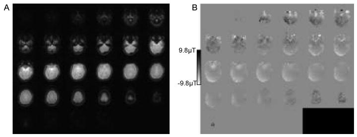
Example navigator volumes. A. Magnitude images for first echo, and B. Unwrapped and masked field map with the contrast range doubled (-2π to 2π) due to the phase unwrapping.

The linewidth and S/N, as measured by LCModel, were compared for the different sequences. The VOI for all the scans was in the right central white matter. Figure 8A and B present the mean (+/- one standard deviation) of the S/N and linewidth for each of the different SVS protocols calculated over all the volunteers. There is no loss in S/N due to the navigator and no increase in linewidth when using real-time shim and motion correction (ShMoCo) for both stationary and moving scans. When no shim correction was applied to the scans with movement, the linewidth increases on average by approximately 2 Hz while the variability of linewidths increases dramatically with no motion correction. The S/N is 33% lower (significance p < 0.05) when no shim correction is applied to the scans with movement. Figure 9 shows the spectra for all the scans acquired with movement (fully shim and motion corrected, motion corrected only, and uncorrected scans) for each of the six volunteers superimposed on top of the respective baseline scan without movement. These plots demonstrate that the spectra are affected by the pose change when no correction and only motion correction are applied.

Figure 8.

A. Bar graph of the mean signal to noise ratio (S/N as calculated by LCModel, +/- one standard deviation). B. Bar graph of the mean linewidth (+/- one standard deviation). Both calculated over the 6 volunteers for each of the three stationary baseline scans and each of the three acquisitions with motion.

Figure 9.

Spectra obtained in the right central white matter for the three scans acquired with movement (no correction, with motion correction, and with full shim and motion correction) for all six volunteers superimposed on top of the respective baseline spectra with no navigator. The plots are the spectra as fitted by LCModel.

The motion and shim estimates measured as a function of time by the vNav for one of the acquisitions with motion and motion correction only is presented in Figure 10. As no shim correction was applied during the scan, the plotted VOI frequency shift was computed using an offline spectral cross-correlation of each FID acquired in the scan to the first FID. The first-order shim estimates have been offset by their values at data point 3 for ease of comparison. As frequency and shim were measured regardless of whether such feedback was applied, Figure 11A and B present scatter plots of the frequency and Y-axis shim change for all three scans with movement in all six volunteers as a function of the angle of rotation about X due to the chin up movement. The Y shim gradient is plotted here as it was affected most by this movement as seen in Figure 10C. These frequency, shim, and head rotations, were measured for the maximum chin-up rotation, averaged over the duration that the subject maintained that pose. These scatter plots demonstrate a correlation of frequency and shim with head pose. For the Y axis shim, the trend is roughly a 1° to 1 μT/m (y = 0.99θ + 0.6) relationship between the head up down angle and Y shim gradient.

Figure 10.

Navigator output and frequency variation from the motion corrected acquisition of volunteer 6. A. Absolute motion estimate as calculated by the navigator, B. mean VOI frequency as calculated from FID cross-correlation, and C. first-order B0 shim change as calculated by the navigator, all as a function of the TR over the duration of the acquisition. X, Y, and Z refer to the scanner axes perpendicular to the sagittal, coronal, and transverse planes, respectively.

Figure 11.

A. Scatter plot of change in frequency and B. change in Y shim gradient as a function of the angle of chin-up rotation about X for all three scans with motion from the six volunteers as measured by the vNav. These values were calculated form the maximum chin-up rotation, averaged over the duration that the subject maintained that pose.

To decouple the effect of frequency shift from first-order shim changes on line broadening, the three scans with movement for three of the volunteers (4, 5, and 6) were processed offline to remove frequency shifts by cross-correlating the spectrum of each FID to that of the first FID and producing a new frequency-coherent average for each scan. These frequency-coherent averages had a mean linewidth (± one standard deviation) averaged across the three volunteers of 4.9 ±0 Hz with shim and motion correction, 6.8 ±0.9 Hz with only motion correction, and 6.5 ±0.5 Hz when no real time correction is applied. This demonstrates a loss in linewidth purely as a result of first-order shim changes, independent of frequency shifts, of just under 2 Hz when no shim correction is applied.

For the three additional SVS scans acquired in the medial frontal lobe of volunteer 5, the scan with motion, and shim and motion correction, had the same linewidth and S/N as the baseline stationary scan, namely 4.9 Hz and 20, respectively. By comparison, the moving scan with only motion correction had a linewidth of 6.8 Hz and S/N of 14. The chin-up rotation produced a shim change in Y of 10 μT/m while the chin-left rotation produced the same shim change in Y of 10 μT/m and additionally a 15 μT/m change in X, both calculated as the mean during the respective pose.

Discussion

Single voxel spectroscopy is a technique that inherently lacks anatomical information and thus accurate volume localisation cannot be guaranteed. Furthermore, the accuracy of the spectra may be adversely affected by artefacts induced by pose change, including phasing errors, line broadening and frequency drifts over time that may or may not be observable.

The changes in B0 resulting from changes in pose are dependent on the region of interest. As Figure 5 demonstrates, all four VOI's exhibited a frequency and first-order B0 change with both chin-down to -up and left to right movements, however, first-order B0 changes were not significant in the right central region for left to right pose change. The second-order B0 shimming requirements are significant in the frontal lobe and as such the ability to adapt these second-order shim terms in relation to pose changes would be beneficial, although it is not possible on the current hardware.

In this work a vNav capable of measuring head pose and B0 shim correction factors within a single TR was demonstrated. This vNav is ideal for spectroscopy as it provides a series of anatomical images with sufficient resolution to provide online pose estimation and offline registration of the spectra to an anatomical image. The accuracy of the volume-to-volume registration performed by PACE was not scrutinised in this study, however, the baseline fluctuations in position estimates were well below 1 mm and 1°. Two sources of image artefact in the vNav are: the presence of dark bands resulting from the three PRESS slice selection planes, and image distortions due to the use of a spectroscopy-specific shim. The impact of the dark bands is minimised by the use of SVS water suppression; the water suppression perturbs globally the magnetisation of the entire volume thus minimising the dark bands. The second is inherently corrected by the navigator after the first TR by applying the appropriate first-order shim for the vNav as calculated from the vNav itself and thereafter alternately switching the shim between the best calculated values for the navigator and the best values for the spectroscopy VOI.

The first question investigated in this study was whether the navigator impacted the signal of the spectra. S/N measurements in LCModel demonstrated that the vNav had no effect on the S/N compared to acquisitions with no navigator (shown in Figure 8). It should be noted that a change in TR from 2 s to 1.5 s would have a noticeable effect on this S/N. The accuracy of the navigator's shim estimate is demonstrated by the linewidth of the baseline acquisitions with real-time shim correction where the mean and standard deviation did not exceed that of the manually optimised shim.

This vNav technique provides three real-time adjustments: VOI location, frequency, and first-order shim correction. The benefit of applying all three is clearly demonstrated by the narrow linewidth and high signal to noise in the presence of pose change (Figure 8). The effect of shim adjustment and VOI localisation correction was decoupled by acquiring an acquisition with only motion correction. In order to separate the effects of frequency shifts from first-order shim errors on linewidths, offline frequency correction was applied to motion corrected data of 3 subjects. While the linewidth improved with each adjustment, it was only fully regained by applying all three.

In the data presented, each subject's chin was raised for approximately 1/3 of the acquisition and resulted in a mean linewidth increase from 4.9 Hz to 6.8 Hz when offline frequency correction was applied. This is consistent with eq. 1 which suggests that for the duration of a 10 μT/m shim change, the linewidth will increase from 5 Hz to 10 Hz. As this only occurred for 1/3 of the acquisition in the present case, the mean linewidth is expected to be 5 Hz + (5 Hz/3) = 6.7 Hz. The use of offline frequency correction demonstrated an improvement in linewidth due solely to shim correction and not due to frequency correction. This is because a single frequency shift, as is present in our data, results in a secondary peak, rather than line broadening.

The real-time shim data and results presented here are the raw estimates from a single navigator. One could further increase the stability of the navigator by taking into account the large time course of data available. This type of temporal filtering would prove beneficial should an accelerated version of the navigator be implemented.

The three scans in the medial frontal grey matter of volunteer 5 demonstrate the application of the vNav in a region of higher B0 inhomogeneity. In such regions a higher vNav spatial resolution provides the specificity required for first-order shim measurements. This higher resolution vNav protocol has a limited FOV that requires the operator to position the vNav over the subject's brain. This additional step should be taken into account when choosing the appropriate vNav protocol for the VOI. This scan demonstrated significant first-order shim changes for both chin-up and chin-left rotations indicating the importance of this type of navigator in regions of high B0 inhomogeneity.

As already discussed, the navigator is dynamically configurable and should a shorter TR be necessary, simply reducing the number of partitions acquired and subsequently manually positioning the navigator over the anatomy of interest enables TRs of 1.5 s to be achieved. Acquiring the complete scanner FOV with the navigator simplifies the user interaction and was achievable with our TR of 2 s. The duration of the complete navigator block presented is approximately 1.1 s and is faster than that achieved using the PROMO technique in SVS (8) of 1.5 s. Further navigator optimisation is possible by employing acceleration techniques like parallel imaging.

Finally, this work has not addressed phasing errors brought about by subject movement during the PRESS localising gradients. Reacquisition, as presented by Zaitsev (7) would be one possible solution, however, as single voxel spectra are accumulated over repeated measurements it may be more appropriate to provide an offline tool to simply exclude dephased measurements.

Conclusion

Changes in B0 homogeneity were demonstrated in four different SVS VOI's in a single volunteer for different head poses. A volume navigator capable of measuring and adjusting, in real time within each TR, head pose, VOI frequency, and VOI first-order shim has been demonstrated. For restless subjects whose head pose cannot be assumed to be constant, this provides a useful addition to the SVS sequence. The first-order shim estimates calculated by the vNav result in linewidths equal to those achieved with manual first-order shim optimisation and maintain spectral quality in the presence of pose changes.

References

- 1.Ernst T, J L. Phase navigators for localized MR spectroscopy using water suppression cycling. Proceedings of the 17th annual meeting of the ISMRM; Honolulu, HI. 2009. p. 239. [Google Scholar]
- 2.Helms G, Piringer A. Restoration of motion-related signal loss and line-shape deterioration of proton MR spectra using the residual water as intrinsic reference. Magnetic Resonance in Medicine. 2001;46(2):395–400. doi: 10.1002/mrm.1203. [DOI] [PubMed] [Google Scholar]
- 3.Posse S, Cuenod CA, Le Bihan D. Motion artifact compensation in 1H spectroscopic imaging by signal tracking. Journal of Magnetic Resonance Series B. 1993;102:222. [Google Scholar]
- 4.Star-Lack JM, Adalsteinsson E, Gold GE, Ikeda DM, Spielman DM. Motion correction and lipid suppression for 1H magnetic resonance spectroscopy. Magnetic Resonance in Medicine. 2000;43(3):325–30. doi: 10.1002/(sici)1522-2594(200003)43:3<325::aid-mrm1>3.0.co;2-8. [DOI] [PubMed] [Google Scholar]
- 5.Henry PG, van de Moortele PF, Giacomini E, Nauerth A, Bloch G. Field-frequency locked in vivo proton MRS on a whole-body spectrometer. Magnetic Resonance in Medicine. 1999;42(4):636–42. doi: 10.1002/(sici)1522-2594(199910)42:4<636::aid-mrm4>3.0.co;2-i. [DOI] [PubMed] [Google Scholar]
- 6.Thiel T, Czisch M, Elbel GK, Hennig J. Phase coherent averaging in magnetic resonance spectroscopy using interleaved navigator scans: Compensation of motion artifacts and magnetic field instabilities. Magnetic Resonance in Medicine. 2002;47(6):1077–82. doi: 10.1002/mrm.10174. [DOI] [PubMed] [Google Scholar]
- 7.Zaitsev M, Speck O, Hennig J, Büchert M. Single-voxel MRS with prospective motion correction and retrospective frequency correction. NMR in Biomedicine. 2010;23(3):325–32. doi: 10.1002/nbm.1469. [DOI] [PubMed] [Google Scholar]
- 8.Keating B, Deng W, Roddey JC, White N, Dale A, Stenger VA, Ernst T. Prospective motion correction for single-voxel 1H MR spectroscopy. Magnetic Resonance in Medicine. 2010;(64):672–9. doi: 10.1002/mrm.22448. [DOI] [PMC free article] [PubMed] [Google Scholar]
- 9.Fu ZW, Wang Y, Grimm RC, Rossman PJ, Felmlee JP, Riederer SJ, et al. Orbital navigator echoes for motion measurements in magnetic resonance imaging. Magnetic Resonance in Medicine. 1995;34(5):746–53. doi: 10.1002/mrm.1910340514. [DOI] [PubMed] [Google Scholar]
- 10.Welch EB, Manduca A, Grimm RC, Ward HA, Jack CR., Jr Spherical navigator echoes for full 3D rigid body motion measurement in MRI. Magnetic Resonance in Medicine. 2002;47(1):32–41. doi: 10.1002/mrm.10012. [DOI] [PubMed] [Google Scholar]
- 11.van der Kouwe AJW, Benner T, Dale AM. Real-time rigid body motion correction and shimming using cloverleaf navigators. Magnetic Resonance in Medicine. 2006;56(5):1019–32. doi: 10.1002/mrm.21038. [DOI] [PubMed] [Google Scholar]
- 12.White N, Roddey C, Shankaranarayanan A, Han E, Rettmann D, Santos J, Kuperman J, Dale A. PROMO: Real-time prospective motion correction in MRI using image-based tracking. Magnetic Resonance in Medicine. 2010;63(1):91–105. doi: 10.1002/mrm.22176. [DOI] [PMC free article] [PubMed] [Google Scholar]
- 13.Webb P, Spielman D, Macovski A. Inhomogeneity correction for in vivo spectroscopy by high-resolution water referencing. Magnetic Resonance in Medicine. 1992;23(1):1–11. doi: 10.1002/mrm.1910230102. [DOI] [PubMed] [Google Scholar]
- 14.Reese TG, Davis TL, Weisskoff RM. Automated shimming at 1.5 T using echo-planar image frequency maps. Journal of Magnetic Resonance Imaging. 1995;5(6):739–45. doi: 10.1002/jmri.1880050621. [DOI] [PubMed] [Google Scholar]
- 15.van der Kouwe AJW, Benner T, Salat DH, Fischl B. Brain morphometry with multiecho MPRAGE. Neuroimage. 2008;40(2):559–69. doi: 10.1016/j.neuroimage.2007.12.025. [DOI] [PMC free article] [PubMed] [Google Scholar]
- 16.Ashburner J. A fast diffeomorphic image registration algorithm. Neuroimage. 2007 Oct 15;38(1):95–113. doi: 10.1016/j.neuroimage.2007.07.007. [DOI] [PubMed] [Google Scholar]
- 17.Thesen S, Heid O, Mueller E, Schad LR. Prospective acquisition correction for head motion with image-based tracking for real-time fMRI. Magnetic Resonance in Medicine. 2000;44(3):457–65. doi: 10.1002/1522-2594(200009)44:3<457::aid-mrm17>3.0.co;2-r. [DOI] [PubMed] [Google Scholar]
- 18.Jenkinson M. Fast, automated, N-dimensional phase-unwrapping algorithm. Magnetic resonance in medicine. 2003;49(1):193–7. doi: 10.1002/mrm.10354. [DOI] [PubMed] [Google Scholar]
- 19.Bottomley PA. Spatial localization in NMR spectroscopy in vivo. Annals of the New York Academy of Sciences. 1987;508:333. doi: 10.1111/j.1749-6632.1987.tb32915.x. [DOI] [PubMed] [Google Scholar]
- 20.Provencher SW. Estimation of metabolite concentrations from localized in vivo proton NMR spectra. Magnetic Resonance in Medicine. 1993;30(6):672–9. doi: 10.1002/mrm.1910300604. [DOI] [PubMed] [Google Scholar]