UNMIX modeling of ambient PM_2.5 near an interstate highway in Cincinnati, OH, USA

Abstract

The “Cincinnati Childhood Allergy and Air Pollution Study (CCAAPS)” is underway to determine if infants who are exposed to diesel engine exhaust particles are at an increased risk for atopy and atopic respiratory disorders, and to determine if this effect is magnified in a genetically at risk population. In support of this study, a methodology has been developed to allocate local traffic source contributions to ambient PM_2.5 in the Cincinnati airshed. As a first step towards this allocation, UNMIX was used to generate factors for ambient PM_2.5 at two sites near at interstate highway. Procedures adopted to collect, analyze and prepare the data sets to run UNMIX are described. The factors attributed to traffic sources were similar for the two sites. These factors were also similar to locally measured truck engine-exhaust enriched ambient profiles. The temporal variation of the factors was analyzed with clear differences observed between factors attributed to traffic sources and combustion-related regional secondary sources.

1. Introduction

The fine fraction of the atmospheric aerosol has been receiving significant attention in recent years due to its potential impact on human health and the environment. Several toxicological and epidemiological studies have confirmed the relationship of exposure of particles to human health (Brunekreef et al., 1997; Dockery et al., 1993; Saxon and Diaz-Sanchez, 2000; Schwartz et al., 1996). There are several studies that have also indicated the cofounding effects of anthropogenic aerosols (such as industrial emissions, traffic exhausts) and naturally occurring bioaerosols in respiratory disorders (Nel et al., 1998; Takenaka et al., 1995). Emissions from traffic-related sources in urban areas have been examined by several researchers (Cadle et al., 1999;Gillies and Gertler, 2000; HEI, 2002; Schauer et al.,1996; Shi et al., 1999). A large cohort epidemiological study is underway in the Greater Cincinnati area to examine the adjuvant role of traffic related and naturally occurring aerosols on enhancing the onset of allergic sensitization in children (LeMasters et al., 2003; Ryan et al., 2004).

The Greater Cincinnati area was recently designated as non-attainment for the PM_2.5 National Ambient Air Quality Standard. The region ranks 24th amongst 401 urbanized areas in the USA in total miles of interstate highways, and has a large volume of heavy duty freight vehicles that travel on these highways (FHWA, 2001). Cincinnati is also a heavily industrialized area. Thus, it is important to identify contributions of the different source categories to support epidemiological studies and develop sound policy and abatement actions. An extensive ambient sampling study was initiated to establish the spatial variations of 24-h integrated PM_2.5 concentration and its constituents (Martuzevicius et al., 2004). In addition, an intensive sampling study was conducted with several real time instruments to elucidate temporal variations and establish variances in size distributions and morphology of the ambient aerosols (McDonald et al., 2004).

Various receptor modeling approaches have been used to unravel the contributions of important source categories to observed ambient concentrations. Several factor-based approaches have been used, including principal component analysis (PCA) followed by multiple linear regression (MLR) (Larsen and Baker, 2003), positive matrix factorization (PMF) (Paatero and Tapper, 1994) and UNMIX (Henry, 2000). UNMIX has been recently utilized to establish ambient aerosol sources and was reported to provide good agreement with predictions of other multivariate receptor models (e.g. PCA/MLR, PMF), especially in identifying the dominant source categories (Henry, 2000; Lewis et al., 2003; Larsen and Baker, 2003; Maykut et al., 2003; Mukerjee et al., 2004). A summary of various recent UNMIX applications are outlined in Table 1. Chen et al. (2002) conducted a UNMIX analysis of speciated PM_2.5 data in the Fort Meade, MD area. The investigators obtained a factor that was attributed to a composite mobile source with an elemental carbon (EC) to organic carbon (OC) ratio of 0.55. They reported that this factor more closely resembled gasoline-fueled vehicle emissions than diesel-fueled ones. Lewis et al.(2003) carried out a similar UNMIX analysis for speciated data obtained in Phoenix, AZ. The authors delineated between gasoline and diesel engine sources; the EC/OC ratio for the diesel source was 0.66, whereas it was 0.32 for the gasoline sources. Maykut et al. (2003) and Kim et al. (2004) reported UNMIX results for the Seattle, WA area. Maykut et al. (2003) reported that carrying out the analysis with EC and OC components resulted in a composite traffic factor. However, by using subfractions of OC and EC from the temperature programmed thermooptical analysis, they could delineate between gasoline and diesel engine sources.

Table 1.

Summary of recent UNMIX applications reported in the literature

	Dataset	Time frame and no. of samples	Location	Identified major source categories	Reference
1	Hourly concentrations of 37 C2-C9 volatile organic compounds (VOC)	Summer, 1990 (550)	Downtown Atlanta, GA, USA	Vehicles in motion; evaporation of whole gasoline; gasoline headspace vapor	Henry (1994)
2	PM2.5 (total mass, sulfate, nitrate, ammonium, OC, EC, Se, Br and Cu)	July 1999-2001 (>200)	Fort Meade, MD, USA	6 sources: regional sulfate; Se/sulfate; secondary nitrate/mobile; summer mobile; wood smoke; Cu/Fe/sulfate	Chen et al. (2002)
3	PM2.5 (Al, Si, S, K, Ca, Mn, Fe, Br, OC, EC and Kw—potassium from wood burning)	March 1995-June 1998 (789)	Phoenix, AZ, USA	Gasoline; diesel; secondary sulfate; crustal/soil; vegetative burning	Lewis et al. (2003)
4	Gas- and particle-phase polycyclic aromatic hydrocarbons (PAHs)	March 1997-December 1998 (61)	Baltimore, MD, USA	4 sources: vehicle; coal; oil; other/wood	Larsen and Baker (2003)
5	Non-methane hydrocarbon (NMHC)	4 seasons in 2001 (84, 84, 48, 59)	Helsinki, Findland	4 sources: gasoline exhaust; liquid gasoline; distant sources, others	Hellén et al. (2003)
6	PM2.5 (H, ${\mathrm{SO}}_4^{2-}$, Si, Al, Fe, Ca, V, Ni, K, Pb, OC2, OC3, OC4, EC1)	1996-1999 (289)	Central urban site, Seattle, WA, USA (same as Kim et al. (2004))	6 sources: Gasoline; diesel; vegetative; fuel oil; soil and Marine	Maykut et al. (2003)
7	Hourly averaged size distribution (16 size intervals from 20 to 400 nm)	December 2000-February 2001 (1051)	Central urban site Seattle, WA, USA (same as Maykut et al. (2003))	Wood burning; secondary aerosol, diesel emissions and motor vehicle emissions	Kim et al. (2004)
8	PM10 (Na, Mg, Ti, Al, Ba, Cu, Fe, Zn, Ca, K, Sb)	April-September 2001 (165)	5 sites near a municipal solid waste incinerator of Toulon (South of France), coastal environment	4 sources determined and further verified by meteorological data	Floch et al. (2003)
9	Ambient VOCs	November 1999-December 1999 (220)	Central EL Paso, TX, near the US-Mexico Border	3 sources: motor vehicle exhaust, gasoline vapor evaporation, liquefied propane gas	Mukerjee et al. (2004)

While numerous receptor modeling studies have been conducted, this is the first known study on the PM2.5 fraction in the Greater Cincinnati area. Furthermore, it has been conducted in support of a large epidemiological study. Hence, the procedure aspects of receptor modeling, with features such as smaller seized datasets (due to budgetary considerations) and incomplete speciated information that are common to several epidemiological studies, are addressed.

In this study, UNMIX analysis was performed on speciated ambient PM_2.5 aerosols using US ESPA UNMIX v2.3. One site (of two such sites in the Cincinnati area) was operated by a local monitoring agency according to the Speciation Trends Network (STN) protocols. The other site was established specifically for the Cincinnati Childhood Allergy and Air Pollution Study CCAAPS study. It operated on a different sampling schedule than the STN protocol site and included a subset of the STN-measured species. Despite these differences, the two sites provide an opportunity to compare and contrast the factors obtained from UNMIX and the inferred traffic source contributions.

2. Methods

2.1. Sampling locations

The entire epidemiological study involved sampling at 24 sites of the CCAAPS network and 10 additional PM_2.5 monitoring stations operated by Hamilton County Department of Environmental Service (HCDOES); however, the data for this paper were collected at two sites: Findlay and Lower Price Hill (Fig. 1). These two sites span interstate highway I-75, a heavy traffic corridor in the Greater Cincinnati area. The Findlay site is located at 940 Findlay Street, Cincinnati, OH, about 210 m east of I-75. This site was established to support the CCAAPS study. The Lower Price Hill (LPH) site is located at 2101 West Eighth Street, Cincinnati, OH, about 1.7 km southwest of I-75. This site is operated by HCDOES as part of the national urban speciation trends network (STN). The distance between these two sites is about 2.2 km.24-h integrated ambient air sampling was conducted nominally 0900-0900 (+1 day) ELT (local time) at Findlay and 0000-0000 (+1 day) EST at LPH. A detailed summary of the sampling dates at the two locations is provided in Table 2.

Fig. 1.

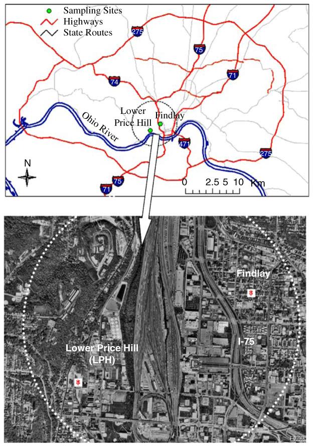
Schematic diagram and aerial photograph of study area.

Table 2.

Description of the sampling schedule and total samples analyzed

Site	Description	Sampling			Total samples
					XRF	EC/OC	Ions
Findlay	Downtown Cincinnati area. 210 m east of I-75	2002	March	18, 19, 20, 21, 26, 27, 28	7	Null	Null
			April	1, 2, 3, 5a,b, 10a, 11a, 12, 15, 16, 17, 18, 22, 23, 24, 25	15	3
			May	28, 29, 30	3	Null
			June	3, 4, 5, 6, 10a, 11a, 12a, 13a, 17a,b, 18a	10	6
			July	24a, 25a	2	2
			August	27, 28, 29	3	Null
			September	9, 10, 11c, 12c, 16a,c, 17a	6	2
			November	7a, 8a, 9a, 11a, 12a, 13a, 14a, 15a, 16a,b, 18a, 19a, 20a,b	12	12
		2003	April	21, 22, 23, 24, 28a, 29a	6	2	Null
			June	23, 24, 25, 26, 30a	5	1
			July	1a	1	1
			October	6, 7, 8, 9, 13a, 14a	6	2
		2004	January	12, 13, 14, 15, 20a	5	1	Null
			March	15, 16, 18, 22a, 23a	5	2
			August	23, 24, 25, 26, 30a, 31a	6	2
			November	29a, 30a	2	2
			December	1a	1	1
Total					95	39	Null
LPH	Downtown Cincinnati area. 1.7 km southwest of I-75	2002	August	6, 12b, 18, 24, 30	5	5	5
			September	5, 11, 17, 23, 29	5	5	5
			October	5, 17b, 23, 29	4	4	4
			November	10	1	1	1
			December	28	1	1	1
		2003	January	3b, 9, 15, 21, 27	5	5	5
			February	2, 8, 14, 20, 26	5	5	5
			March	10, 16b, 22, 28	4	4	4
			April	3, 9, 15, 21, 27	5	5	5
			May	3, 9, 15, 21, 27	5	5	5
			June	2, 8, 14, 20, 26b	5	5	5
			July	2, 8b, 14, 20, 26	5	5	5
			August	7, 13, 19, 25b, 31b	5	5	5
			September	6, 24, 30	3	3	3
			October	6, 12, 18, 24, 30	5	5	5
			November	5, 11, 17, 23, 29	5	5	5
Total					68	68	68

Missing data at LPH are not reported in this Table.

Underlined data were collected on Saturday.

Strikethrough data were excluded from UNMIX runs.

^aCollocated Quartz and Teflon filters used for sampling. EC and OC are determined by NIOSH 5040 method.

^bSamples showed poor mass closure.

^cSamples showed higher levels of Pb and Zn.

To obtain information on source emissions from diesel engines, sampling was also performed near truck weigh stations and at a school bus depot. At the weigh station, trucks with a prepass do not enter the weigh station and run on the interstate highway at a speed of about 60 mph; others are diverted from the highway and go through the station. The PM_2.5 samplers were set about 1 m away from the scale where the trucks were weighed and 12 m from the interstate highway. Sampling was conducted during an 8-h period. The school bus depot sampling location had about 100 buses with engines warming up prior to daily runs. The PM_2.5 samplers were operated for about 4 h at this location. The equipment and analysis methods used for the ambient air sampling at Findlay were also adopted for these diesel emissions-enriched ambient measurements as described in the next section.

2.2. Sampling and analysis methods

The details of the sampling and analysis methods adopted for the CCAAPS study and those used at the Findlay site are described elsewhere (Martuzevicius et al., 2004), only a brief description is provided here. PM_2.5 samples were collected on 37-mm Teflon membrane filters (nominal pore size = 1 μm) (Pall Corporation, Ann Arbor, MI, USA) and 37-mm quartz filters (Whatman Inc., Clifton, NJ, USA) with Harvard-type Impactors (Air Diagnostics and Engineering Inc., Harrison, ME). The Teflon filters were conditioned for at least 24 h in a humidity chamber for temperature and humidity equilibration at Washington University in St. Louis (WUSTL) and weighed before and after the sampling to determine PM_2.5 mass concentrations. The Teflon filters were then analyzed by X-ray fluorescence (XRF) to determine elemental concentrations (Chester Labnet, Tigard, OR). 15 chemical species (Al, Si, S, K, Ca, Ti, Cr, Mn, Fe, Ni, Cu, Zn, Se, Br, Pb) were consistently observed to be present. The quartz filters were sectioned with one half analyzed by the Thermal-Optical Transmittance (TOT) technique using the NIOSH-5040 method (Birch and Cary, 1996) to determine EC and OC concentrations (Sunset Lab, Hillsborough, NC). The other half was frozen and preserved. Field and laboratory blanks were routinely analyzed, with details reported elsewhere (McDonald, 2003).

At Lower Price Hill (LPH), 24-h integrated PM_2.5 samples were collected every 6th day using a SASS sampler (Met One Instruments Inc., Grants Pass, OR). The LPH site is part of the State and Local Air Monitoring Station (SLAMS) network. Mass and speciation analysis were performed by RTI (Research Triangle Park, NC) following protocols adopted by the EPA Speciation Trend Network (STN). Table 2 provides a summary of the measurements and analyses.

The CCAAPS baseline monitoring platform (used at the Findlay site) initially consisted of Teflon filter sampling with only periodic sampling on quartz filters. Given the importance of EC to this study, an optical reflectance method was used to estimate the EC concentrations from the Teflon filters. The reflectance of ambient aerosols deposited on the Teflon filter was measured by a reflectometer (EEL model 43; Diffusion System Ltd., London, UK). The absorption coefficient (A_bs) of the aerosol-loaded Teflon filters was calculated according to international standard ISO 9835 (1993):

$$A_{\mathrm{bs}}=\left(\frac{A}{2V}\right)\ln \left(\frac{R_{\mathrm{b}}}{R_{\mathrm{s}}}\right),$$ (1)

where R_s is the normalized reflectance of the sample filter as a percentage of the reflectance of a clean control filter (100 by definition); R_b is the average of the normalized reflectance of the field blank filters; V is the air volume sampled (m³); and A is the area of the deposit on the filter (m²). The absorption coefficient was correlated with EC from NIOSH 5040 thermooptical transmittance analysis for days when quartz filter sampling was conducted.

The meteorological parameters—wind direction, wind speed, temperature and humidity—were recorded with 5 min resolution with a Vantage Pro Weather Station (Model 6150, Davis Instruments, Baltimore, MD) that was located beside the PM_2.5 sampler, at a height of 2 m above the ground.

3. UNMIX model calculations

Chemical Mass Balance (CMB) models have been extensively used by researchers; however, these models require a priori knowledge of source profiles. While some receptor modeling studies have been previously conducted in the Cincinnati area (Mukerjee and Biswas, 1992; Mukerjee and Biswas, 1993; Shenoi, 1990), detailed local source profiles are not available for PM_2.5 constituents. The UNMIX, multivariate model (Henry, 1994, 2003;Henry et al., 1999) was adopted in this study to derive factors which presumably can be attributed to emission source categories. To our knowledge this is the first application of a receptor modeling study of PM_2.5 constituents in the Greater Cincinnati area.

UNMIX utilizes highly dimensional ‘edges’ of data points in conjunction with non-negative constraints on both source profiles and contributions to find the number of sources and their respective species profiles solely based on the measured data (Henry, 2003). The first step adopted is applying ‘NUMFACT’ (Henry et al., 1999) to determine the number of influencing sources. This is analogous to factor analysis methods that establish the number of factors (or sources), but with different criteria being invoked. Singular value decomposition (SVD) is then performed on the normalized measured chemical concentration data to reduce the dimensionality with respect to the retained number of factors (or sources). The edges of the data set are established which are then used to determine the source profiles. Contributions of these source categories can be calculated using the singular value decomposition model as demonstrated by Henry (2003).

The steps that are adopted in this work in running the UNMIX model are the following (Henry, 2000):

1. Species were excluded as fitting species if their average ratio of the concentration to the uncertainty was less than two;

2. Organic carbon at Findlay was blank-corrected by subtracting the study-averaged trip and field blank OC level from the routine (24 h-integrated) sampled OC. This blank correction was equal to 0.90±0.39 μg m^-3. Both EC and OC at LPH were blank-corrected by the study-average field blank levels of 0.15±0.07 μg m^-3 for EC and 1.36±0.43 μg m^-3 for OC. Negative artifacts were not considered since there was no available data;

3. Mass reconstructions were used to screen the data as outlined by Malm et al. (1994), Tolocka et al. (2001), Chen et al. (2002), and Lewis et al. (2003). The following weights were used to adjust the measured species to an assumed compound or bulk composition: S concentrations were multiplied by 4.13 which assumes that all the sulfur species are present as ammonium sulfate; Al, Si, Ca, a portion of Fe, and Ti are assumed to be of crustal origin and are multiplied by 2.20, 2.49, 1.63, 2.42 and 1.94, respectively, corresponding to their major oxides. Organic carbon concentrations after blank correction were multiplied by 1.4 as an estimate of total organic matter;

4. Scatter plots were used to establish relationships between each species and the PM_2.5 mass concentration. These plots were used to determine the “good edge” species;

5. Initial runs of UNMIX with these “good edge” species identified the set of contributing sources such that at least 80% of variance of each species could be explained by these sources. The set of factors that accounted for the greatest variance of the species was selected, along with the highest signal-to-noise ratio (greater than two is recommended);

6. Follow up runs were performed with additional species to ensure stability and to search for feasible solutions with a larger number of sources; and

7. Edge plots were used to guarantee sufficient number of points to define the edges for each source. Those points forming poor edge were excluded from the UNMIX runs.

4. Results and discussion

4.1. Average ambient concentrations

Mass concentrations for PM_2.5 and its chemical components at the two sites are listed in Table 3. The PM_2.5 concentrations over the entire sampling period reported in this paper were 20.4±9.0 and 17.8±8.1 μg m^-3 at Findlay and the LPH sites, respectively. While the spatial variation in the PM_2.5 mass concentration is rather low (Martuzevicius et al., 2004), there was a significant temporal variation (approximately 44% with respect to the mean concentration). The difference in mean PM_2.5 levels (20.4 compared to 17.8 μg m^-3) at the two sites might arise from the different sampling schedules (Table 2) and/or the differences in sampler hardware and operations. Alternatively, they might reflect actual differences in the long-term PM_2.5 mass concentrations between these sites.

Table 3.

Average PM_2.5 and species concentrations measured at Findlay and LPH^a

	Findlay		LPH
	Mean±SDb	No. of samplesc	Mean±SDb	No. of samplesc
PM	20.4±9.0	95	17.8±8.1	68
	units: μg m-3		units: μg m-3
EC	1.3±0.7	39	0.8±0.5	68
OC	3.9±1.8	39	3.7±1.8	68
${\mathrm{NO}}_3^{-}$	NMc	0	2.0±1.9	68
${\mathrm{SO}}_4^{2-}$	NMc	0	5.5±3.9	68
${\mathrm{SO}}_4^{+}$	NMc	0	2.3±1.3	68

	units: ng m-3		units: ng m-3
Al	57.7±72.1	95	41.8±71.8	44
Si	173.0±156.9	95	122.0±115.9	68
S	1711.2±1030.4	95	1701.8±1151.9	68
K	77.3±40.1	95	122.7±97.5	57
Ca	174.6±105.0	95	59.6±33.1	67
Ti	9.6±6.3	95	6.9±6.8	58
Cr	0.8±0.6	93	2.1±2.2	59
Mn	4.5±2.7	95	3.1±2.0	56
Fe	196.4±126.0	95	105.0±64.5	68
Ni	0.8±0.7	88	1.4±0.8	42
Cu	5.0±4.4	95	4.9±6.0	54
Zn	64.0±113.3	95	22.5±29.4	67
Se	2.5±2.0	94	2.6±1.9	66
Br	5.6±6.0	95	4.3±2.8	61
Pb	9.8±13.1	95	8.9±16.5	59

^aSampling periods: March 2002 through December 2004 at Findlay; and August 2002 through November 2003 at LPH.

^bSD is 1 sigma value.

^cNo. of samples both are those above the method detection limits.

The sulfate ions were the largest contributor to the average PM_2.5 mass concentration, followed by organic carbon (OC). Being located in the Ohio River valley, the region is in the vicinity of numerous coal-fired power plants and hence the domination by sulfate species concentrations. More than half of the PM_2.5 mass arises from the major ions—nitrate, sulfate and ammonium while elemental carbon (EC) and organic carbon (OC) accounted for approximately 25% of the average PM_2.5 mass concentration (Table 3). The ratio of EC to OC has been considered an important indicator for the characterization of diesel- and gasoline-fueled vehicle emissions (Gillies and Gertler, 2000). Box plots of the ratio of the EC to OC are shown in Fig. 2 for the Findlay and LPH sites. At both sites, EC and OC are moderately correlated (r² = 0.75 and 0.60 at Findlay and LPH, respectively). The mean values of EC/OC ratio are 0.36 and 0.21 at the Findlay and LPH sites, respectively. The slightly higher EC/OC ratio at the Findlay site may be due to a relatively greater influence of diesel engine emissions as this sampling site which was closer to the highway than the LPH site. This issue is revisited in the discussion of the UNMIX results.

Fig. 2.

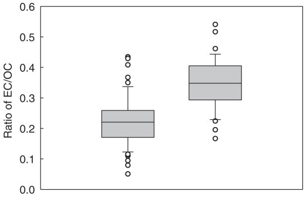
Box plots of EC/OC ratio at Lower Price Hill (N = 68) and Findlay (N = 39). Whiskers represent 5th and 95th percentiles with individual data points outside these thresholds denoted by open circles.

Based on the methods described in the previous section, the reconstructed PM_2.5 mass concentrations from the speciated data were plotted against the measured PM_2.5 mass concentrations, as shown in Fig. 3(A) and (B) for the Findlay and LPH site, respectively. At the Findlay site, these reconstructions include only those samples in which both EC and OC were measured. The reconstructed PM_2.5 varies from 0.44 to 0.99 of the measured PM_2.5 mass concentration. Several factors could cause the low reconstructions, including the exclusion of aerosol nitrate which accounted for 3-40% of the PM_2.5 mass concentration at LPH. At LPH, all major species were routinely measured and most of the samples exhibited reconstructed mass concentrations within 20% of the measured PM_2.5 mass. Data falling outside of these ranges (at Findlay in 2002-5 April, 17 June, 16 and 20 November; at LPH in 2002-12 August, 17 October and in 2003-26 June, 8 July, and 31 August) are shown by “×” markers in Fig. 3.

Fig. 3.

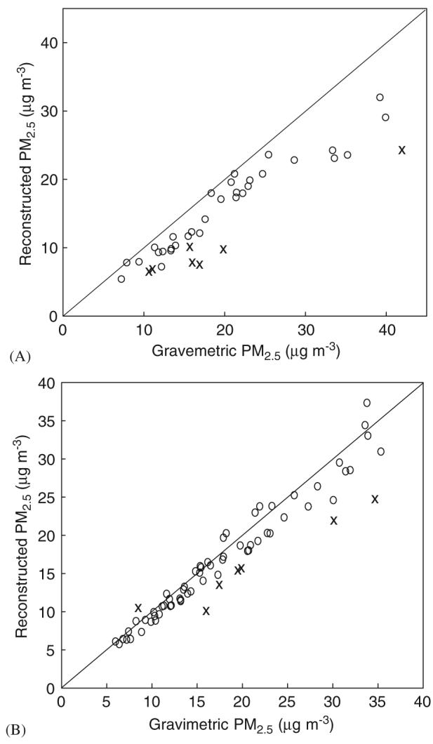
Plot of reconstructed PM_2.5 mass concentrations based on speciated measurements against the gravimetric PM_2.5 mass concentrations: (A) Findlay; and (B) LPH. The solid line is the 1:1 line. Samples deemed outliers for the purpose of UNMIX modeling are denoted by ‘×’.

4.2. Extension of Findlay data set to include EC concentration

For the Findlay data set, EC was directly measured for 39 of the 95 total samples; the balance of these samples included aerosol collection on Teflon filters which precluded ECOC analysis. Since one of the objectives of the study was to delineate the contribution of traffic related sources and because EC is an important indicator of diesel engine exhaust (Schauer, 2002), the data set of EC concentrations was extended using the reflectance method described earlier. The absorption coefficient (A_bs) for each of the 95 samples collected on Teflon filters was determined using Eq. (1) based on reflectance measurements. For the 39 samples with collocated sampling onto quartz filters, the absorption coefficients were correlated to the EC measured by thermo-optical analysis (Fig. 4). A strong linear correlation (r² = 0.91) was obtained and the following calibration equation was determined:

$$\mathrm{EC}\left(\mu \mathrm{g}{\mathrm{m}}^{-3}\right)=0.843\left(A_{\mathrm{bs}}\right)-0.04,$$ (2)

where A_bs has units of 10^-5 m^-1 and EC has units of μg m^-3. Eq. (2) is valid only for this particular location, and should not be universally applied. Eq. (2) was then used with the known values of A_bs from the Teflon filter measurements to estimate EC levels for the 56 days when no quartz filter sampling was conducted. Similar results were also reported in a New York study by Kinney et al. (2000).

Fig. 4.

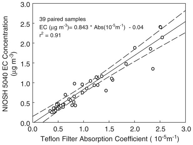
Plot of measured EC concentration (NIOSH 5040 ECOC analysis on quartz filters) against absorption coefficients from reflectance measurements on Telfon filters for collocated samples. Solid line is the best-fit simple linear regression; dashed lines are the 95% confidence levels.

4.3. Scatter plots and UNMIX inputs

Scatter plots have been used in air quality studies as a screening method for selection of fitting species and identifying outliers (Henry, 1994, 2000; Lewis et al., 2003). UNMIX allows the user to generate scatter plots, which was then used as a first step to choose the species potentially contributing to PM_2.5 levels (Henry, 2000). Based on the measurements carried out at Findlay, scatter plots are shown in Fig. 5 for a variety of different species versus PM_2.5 mass. For several species such as Al, Ca, Mn and Fe, the data points are scattered over the entire plane of the plot. However, S shows a strong linear correlation with PM_2.5 (r² = 0.72) and EC and OC exhibit a moderate degree of correlation (r² = 0.30 and 0.52, respectively) with PM_2.5 levels. The data for Pb and Zn are closer to the PM_2.5 axis, where on certain days (11, 12, 16 September 2002) showed relative higher levels, suggesting significant impact of metal processing sources.

Fig. 5.

Scatter plots of various species concentrations (ng m^-3) versus PM_2.5 mass concentration (μg m^-3) for the Findlay site.

Henry (2000) defined a subjective term “good edge” to describe the species that show a clear relation with PM_2.5 concentration with identifiable, sharp lower and upper edges in the scatter plot. Species such as S, Fe, EC, Mn, Ca can be qualitatively classified as those with “good edges” as demonstrated in Fig. 5. These elements—the selection of which is subjective to some degree—were used first to get the minimum source solution from UNMIX. Other species were systematically added in the UNMIX model to improve the source identification. Due to the availability of all major species components at the LPH site, good closure on the mass balance of PM_2.5 was obtained. Given that the Findlay site data includes only a subset of the PM component available at LPH, a sensitivity check was performed for LPH using only Si, S, Ti, Fe, Zn, EC, and OC as the fitting species in the UNMIX model. These LPH model runs explicitly excluded ammonium, nitrate, and PM_2.5 mass to be consistent with the Findlay modeling. Using these two approaches, the contribution of each fitted species to the respective source profiles agreed within the model-estimated uncertainty. Hence, the Findlay model results presented in this paper used Al, Si, S, Ca, Ti, Mn, Fe, Zn, Pb, EC and OC (when available) while the LPH model results used PM_2.5 mass, nitrate, sulfate, ammonium, Si, Ca, Ti, EC and OC. Note that PM_2.5 mass was excluded from the Findlay model runs because the major ions were not directly measured and there was no basis for assuming a nitrate concentration.

4.4. UNMIX results

4.4.1. Findlay site

UNMIX was applied on the 89-day dataset (Table 4) for which EC was estimated from the reflectance measurements. Six days (12 September 2002, 6 October 2003 and 13 and 20 January, 30 and 31 August 2004) had “poor edges” and hence were excluded from the UNMIX runs. By recalculating the SCEs on those days, several species concentrations were underestimated suggesting the impact of additional sources. A stability analysis was performed by removing samples one at a time—to confirm that a converged result was obtained. The factor loadings from 28-day data set with a direct ECOC analysis agreed with the one obtain from 89-day dataset. The averaged source contributions along with 1-sigma uncertainties are reported in Table 4. The ratios of OC to EC for each of the factors from the 28-day dataset were used to estimate source contributions to OC for the remaining days. The normalized source profiles are listed in Table 4.

Table 4.

Averaged source contributions and 1-sigma uncertainties at the Findlay site determined by UNMIX analysis for the 89-day dataset^a,^b,^c and Normalized fraction of the species for potential sources at the Findlay site^d,^e,^f

	Metal processing (S1)		Traffic (S2)		Combustion related sulfate (S3)		Soil/crustal (S4)
	SCE	1-sigma	SCE	1-sigma	SCE	1-sigma	SCE	1-sigma
A. Averaged source contributions and 1-sigma uncertainties at the Findlay site determined by UNMIX analysis for the 89-day dataset
Al	8.4	3.7	12.1	3.6	5.7	4.4	32.7	9.9
Si	28.6	10.1	56.7	11.3	23.1	12.5	66.2	16.7
S	286.1	159.1	394.7	160.8	1014.5	307.1	63.2	65.1
Ca	33.6	11.0	100.3	17.7	31.0	12.8	8.8	9.2
Ti	1.6	0.6	3.8	0.7	2.0	0.8	2.2	0.7
Mn	1.1	0.3	1.9	0.3	0.9	0.3	0.3	0.2
Fe	47.1	11.7	91.7	17.2	33.7	14.3	19.6	6.9
Zn	43.6	9.6	7.0	3.6	0.3	3.1	1.2	3.0
Pb	6.1	1.4	1.4	0.5	0.7	0.4	0.0	0.4
EC	279.0	87.9	622.7	160.3	348.2	157.6	5.2	58.2

B. Normalized fraction of the species for potential sources at the Findlay site
Al	0.003	0.001	0.002	0.001	0.001	0.001	0.057	0.017
Si	0.010	0.004	0.012	0.002	0.003	0.002	0.116	0.029
S	0.100	0.056	0.082	0.033	0.152	0.046	0.111	0.114
Ca	0.012	0.004	0.021	0.004	0.005	0.002	0.015	0.016
Ti	0.001	0.000	0.001	0.000	0.000	0.000	0.004	0.001
Mn	0.000	0.000	0.000	0.000	0.000	0.000	0.001	0.000
Fe	0.017	0.004	0.019	0.004	0.005	0.002	0.034	0.012
Zn	0.015	0.003	0.001	0.001	0.000	0.000	0.002	0.005
Pb	0.002	0.000	0.000	0.000	0.000	0.000	0.000	0.001
EC	0.098	0.031	0.129	0.033	0.052	0.024	0.009	0.102
OC	0.270	—	0.298	—	0.205	—	—	—

^aSamples were collected from March 2002-December 2004 at Findlay.

^bEC were determined by reflectance method.

^cAveraged measured PM_2.5 concentration was 20.5 μg m^-3.

^dContributions to PM_2.5 were estimated by mass reconstruction methods described in the text (S was multiplied by 4.13, OC by 1.4).

^eFraction is normalized to the source contribution estimates to PM_2.5 by each source.

^fAveraged source contribution to OC is estimated using dataset with EC/OC measurements.

The four factors derived by UNMIX contributed 73% to the average PM_2.5 concentration of 20.5 μg m^-3. Nitrate—which was not available for this analysis—is likely a significant contributor to the missing reconstructed mass. A brief description of the four factors is as follows. The first factor accounted for the largest contributions to ambient Pb and Zn levels. This factor also accounted for ∼16% of the ambient sulfur. There are several metal processing facilities near the Findlay site which might be responsible for this factor; they use high temperature coal combustors and thus likely emit SO₂ (US EPA, 2003) and possibly emit sulfate.

The second factor appears to be a traffic source profile with a total contribution of 24% to the measured PM_2.5 levels. Carbonaceous species (OC and EC) are the dominant PM components in this profile. Due to the close proximity of the site to the highway and the high volumes of diesel engine traffic (>20,000 per day), this factor is the highest contributor to EC levels (48%), and is likely strongly influenced (indeed, possibly dominated) by diesel engine emissions. The abundant species in this factor are EC, OC, S, Ca, Fe, Si, Al, Ti, Mn, and these are among the typically measured species in vehicular emissions such as Mg, Al, Si, P, S, Cl, Ca, Fe, Cu, Zn, Br, and Pb as reported by Gillies and Gertler (2000) and Cadle et al. (1999). The ratio of EC to OC for this factor was 0.43 which is much higher than typically reported for gasoline engine emissions. This factor was a dominant contributor of Mn (42%), consistent with the use of Mn-based additives to enhance engine performance (Lewis et al., 2003; Ramadan et al., 2000).

A comparison of this factor loading (at Findlay) was made to measured diesel engine exhaust source profiles (Fig. 6). Some of these profiles were obtained from the literature (HEI, 2002) and the others from measurements made as part of this study at diesel emission-enriched areas using equipment and analytical methods identical to the ambient measurements at Findlay. Reasonable agreement is obtained, providing further evidence that this factor is likely dominated by diesel vehicle emissions. As stated earlier the Findlay site is very close to the highway that has a high volume of truck traffic. The UNMIX derived factor loadings of EC and OC most closely matched the direct truck-enriched profiles measured at a weigh station in the Cincinnati region (Truck CIN, Fig. 6). While OC and S fractions were consistent across the measurements, there was relatively large variation in the EC level.

Fig. 6.

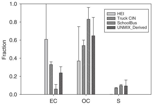
Comparison of UNMIX-estimated traffic source profiles for various diesel engine emissions measurements. Normalized chemical profiles (sum of the identified weight = 1) of EC, OC, and sulfur.

Several PM components were not used in the UNMIX analysis; correlation coefficients for those species with the four UNMIX-generated factors are presented in Table 5. The factor attributed to the traffic source shows moderate correlation with the crustal species Mg (0.49) and K (0.43), which might arise from crustal material resuspended by the movement of large number of heavy duty vehicles.

Table 5.

Correlation coefficients for UNMIX-generated source strengths and the chemical species concentrations not used in UNMIX analysis (Findlay)^a

	Metal processing	Traffic	Regional sulfate	Soil/crustal	Na	Mg	Cl	K	V	Cr	Ni	Cu	Se	Br
Metal processing	1.00	-0.13	-0.23	0.07	0.38	0.05	0.04	0.35	0.28	0.58	0.62	0.68	0.23	0.48
Traffic		1.00	-0.34	-0.02	0.08	0.49	-0.12	0.43	0.23	0.32	0.05	0.28	-0.03	0.20
Regional sulfate			1.00	-0.11	0.13	-0.22	-0.12	0.01	0.12	-0.06	0.01	-0.07	0.31	-0.02
Soil/crustal				1.00	-0.14	0.11	-0.13	0.45	0.14	0.04	-0.10	0.08	0.00	0.01
Na					1.00	0.15	0.29	0.25	0.41	0.41	0.56	0.38	0.08	0.32
Mg						1.00	-0.25	0.21	0.10	0.16	0.24	0.30	-0.13	0.00
Cl							1.00	-0.14	-0.22	-0.05	-0.06	-0.01	0.10	0.20
K								1.00	0.57	0.45	0.14	0.47	0.21	0.36
V									1.00	0.28	0.22	0.25	0.06	0.24
Cr										1.00	0.62	0.66	0.34	0.48
Ni											1.00	0.57	0.23	0.39
Cu												1.00	0.25	0.53
Se													1.00	0.61
Br														1.00

Significant correlations (p<0.05) between species and UNMIX generated source strengths are underlined.

^aSource strength is calculated based on the complete (95-day) data set with reflectance-estimated EC data.

The third factor was a major contributor to measured S levels (greater than 60%), and accounted for 32% (largest) of the ambient PM_2.5. As discussed later, this factor shows significant seasonal day-to-day variation (Fig. 7), and appears to be an indicator for regionally-transported PM with strong contributions from secondary sulfate related to coal combustion. It was also the second largest contributor to the ambient OC concentrations, and had a significant contribution to EC levels. Thus, the factor could be a composite of coal combustion emissions, secondary sulfate, and primary and/or secondary organics. The moderate association with Se (ρ = 0.31) provides additional evidence for attribution of this factor to coal combustion sources.

Fig. 7.

(A) Daily average of PM_2.5 mass contributions (μg m^-3) at Findlay from the UNMIX-generated source profiles. (B) Monthly average PM_2.5 mass contributions (μg m^-3) at Findlay from the UNMIX-generated source profiles.

The fourth factor is the smallest (3%) contributor to the PM_2.5 levels. It is the largest contributor to ambient Si (38%) and showed significant (p<0.05) correlation with several crustal materials such as Mg (0.11) and K (0.45). Thus, this factor appears to be related to resuspended soil or other crustal-related emissions.

Fig. 7 is a time series of the factor-specific contributions to the measured PM_2.5 mass concentrations. Fig. 7a demonstrates that the two dominant factors—attributed to traffic and combustion-related regional sulfate—exhibit significant day-to-day variations. Relatively low contributions from the combustion-related regional sulfate source were observed on several days, such as 1 July, 6 and 7 October 2003; together with a higher contribution from the metal processing source. This is possibly due to the presence of higher concentrations of Zn and Pb in these samples. There is a possibility that the concept of “edges” may fail due to unusually high concentrations of the Zn and Pb species. Monthly average contributions are presented in Fig. 7b with the number of samples reported in the parenthesis below the respective month. While some of these sample subsets are rather small and thus might be at best qualitatively representative of the month, there are stronger contributions from the combustion-related regional sulfate in the summer months compared to the other months. In contrast, traffic source contributions appear to be lowest in the summer months. It is not clear whether this behavior arises from seasonal differences in wind direction dictating the impact of local highway emissions on the site, seasonal differences in mixing height influencing the extent of atmospheric ventilation, or seasonal differences in emissions.

The possible role of near-field (local) emissions on the observed traffic source contributions was investigated for 11 days over a 2-week period in November 2002. Table 6 shows the UNMIX-derived traffic source contribution and the prevailing wind direction as determined from wind roses for each day (listed by the start date). An overall frequency distribution of the 5-min averaged wind direction for this period yielded the following results: 26% from north, 18% from southwest, 15% from west, and 13% from south-southwest. The highest contributions (Table 6) of the traffic source factor occurred on 19 November when the winds arrived from the west for 51% of the sampling period. Moderately high traffic source contributions (Table 6) were also observed on 13 and 14 November which coincided with winds arriving predominantly from the north (68% and 81% of the sampling periods, respectively). These conditions for relatively high traffic source contributions are consistent with the location of the Findlay site where highway I-75 is located both west and north of the site (Fig. 1). A relatively low traffic source contribution was observed on 16 November (Saturday), likely less due to the prevailing meteorological conditions and more due to the lower diesel truck volumes on the weekends. This is consistent with the observation of Lewis et al. (2003) who reported a strong weekend/weekday difference for diesel engine vehicle contributions in Phoenix (0.28 for weekend/weekday). Similarly, the estimated weekend/weekday ratio of traffic source contributions for this Cincinnati study was 0.3. Caution must be exercised in this interpretation as the data is from a limited number of samples, and more weekend samples need to be collected to derive a firm conclusion.

Table 6.

UNMIX estimated traffic source contributions (μg m^-3) at Findlay for November 2002

Date	Prevailing wind direction	UNMIX
7 November 2002	NAa	5.9
8 November 2002	NAa	4.2
9 November 2002	NAa	0.9
11 November 2002	SW	0.6
12 November 2002	SW	1.7
13 November 2002	N	5.3
14 November 2002	N	5.7
15 November 2002	N and W	0.6
16 November 2002	W and S (Variable)	0.5
18 November 2002	W and SW	3.0
19 November 2002	W	16.6

^aNA stands for not available.

4.4.2. Lower Price Hill (LPH) site

Using the procedures described earlier in this manuscript, samples with missing data or those that were determined to be outliers were removed, and a 63-day data set was obtained that was used for UNMIX modeling. The averaged source contributions and the 1-sigma uncertainties are presented in Table 7. This dataset included measurements of ammonium, nitrate and sulfate ions, and much more representative closure on the measured PM_2.5 mass was obtained compared to the Findlay analysis. Four source categories (factors) met the performance measures of the UNMIX model (requiring the variance to be greater than 80%, and signal-to-noise ratio to be greater than 2), and these four sources accounted for 99.1±23.4% of the 63-day sample averaged PM_2.5 concentration of 17.9 μg m^-3.

Table 7.

Averaged source contribution estimates (SCE) (ng m^-3) and 1-sigma uncertainties at the LPH site determined by UNMIX analysis. Normalized fraction of the species at each source is listed in parenthesis^a

	Secondary-nitrate (S1)		Traffic (S2)		Combustion related sulfate (S3)		Soil/crustal (S4)
	SCE	1-sigma	SCE	1-sigma	SCE	1-sigma	SCE	1-sigma
Si	8.9 (0.003)	12.1 (0.004)	19.1 (0.005)	14 0.003	9.2 (0.001)	17.4 (0.002)	82.5 (0.044)	34.6 (0.018)
Fe	11.5 (0.003)	7.4 (0.002)	50.2 (0.012)	11.9 0.003	9.9 (0.001)	9.8 (0.001)	36.1 (0.019)	14.4 (0.008)
Ti	0.6 (0.000)	0.8 (0.000)	-0.4 (0.000)	0.8 0.000	0.6 (0.000)	0.9 (0.000)	5.1 (0.003)	2.1 (0.001)
EC	43.7 (0.013)	34.5 (0.010)	670.1 (0.163)	128.4 0.031	96.4 (0.012)	73.9 (0.009)	44.9 (0.024)	68.2 (0.036)
OC	490.7 (0.148)	169.6 (0.051)	2076.1 (0.505)	473.9 0.115	920 (0.111)	311.5 (0.037)	260.2 (0.138)	241.2 (0.128)
${\mathrm{NH}}_4^{+}$	621.4 (0.187)	126 (0.038)	111.7 (0.027)	102.2 0.025	1312.3 (0.158)	202.4 (0.024)	163.7 (0.087)	129 (0.068)
${\mathrm{NO}}_3^{-}$	1424.7 (0.429)	268.6 (0.081)	166.6 (0.041)	85.5 0.021	106.9 (0.013)	99.3 (0.012)	26.3 (0.014)	86.1 (0.046)
${\mathrm{SO}}_4^{2-}$	616.4 (0.186)	246 (0.074)	91.6 (0.022)	319 0.078	4356.9 (0.524)	675.9 (0.081)	536.9 (0.284)	400.5 (0.212)
PM2.5b,c	3319.7	736.1	4109.5	1086	8315.9	1475.2	1888.7	870.1

^aSamples were collected from August 2002-November 2003 at LPH.

^bAveraged measured PM_2.5 concentration was 17.9μg m^-3 for the 63 days used in analysis.

^cSCEs to PM_2.5 were calculated directly using UNMIX.

The first factor was the largest contributor to ambient nitrate (>71%) and appears to represent a secondary nitrate source. It accounted for about 19.0±4.1% of the total PM_2.5 mass concentration and has ammonium, sulfate and nitrate present in concentrations consistent with the stoichiometry of ammonium nitrate and ammonium sulfate. Fig. 8 shows the monthly average source contributions to the PM_2.5 mass. The secondary nitrate factor shows a strong seasonal variation with highest contributions in the winter and spring, consistent with the conditions that favor ammonium nitrate formation (Seinfeld and Pandis, 1998). A negative correlation of nitrate with temperature (ρ = -0.71) reinforces the seasonal dependence of this factor. The contributions to EC and OC from this factor were companied with relative large uncertainties.

Fig. 8.

Monthly average PM_2.5 mass contributions (μg m^-3) at LPH from the UNMIX-generated source profiles.

The second factor appears to represent traffic sources and accounted for 23.1±6.1% of the total measured PM_2.5 level. This factor was the dominant contributor to both ambient EC and OC. Fig. 8 shows relatively little seasonal variation for this factor. In contrast, Findlay showed lower contributions in the summer compared to the other seasons. These differences might arise from the more uniform data density across months for the LPH site providing a more-robust monthly estimate, or might arise from a weaker sensitivity of the traffic source contributions at LPH compared to Findlay for seasonal differences in meteorological conditions. Unlike Findlay, the sulfur content of traffic profile at LPH showed large uncertainty. This factor exhibited a lower EC/OC ratio (0.32), probably suggesting a weaker diesel vehicle influence to the composite traffic source profile at LPH compared to Findlay. However, the average contribution to EC was about 0.67 μg m^-3 at LPH, comparable to the 0.62 μg m^-3 at the Findlay site. Though the LPH site is at a greater distance from I-75, and probably not influenced as much as the Findlay site by the large number of heavy duty diesel vehicles, there would be other factors causing this comparable traffic source contribution levels, such as the variance of the wind directions and the difference sampling schedules at both sites. Larger data sets with consistent analytes being measured are needed to more-fully investigate differences between the traffic source profiles at LPH and Findlay.

The third factor—a combustion related sulfate source is quite similar to the respective profile for the Findlay site. It is the largest contributor to measured PM_2.5 concentrations, accounting for 46.7±8.3% of the total mass. As at the Findlay site, there was a strong seasonal dependence with highest contributions in the summer. The fourth factor was the smallest contributor (10.6±4.9%) to the measured PM_2.5 levels. It appears to be indicative of resuspended soil or other crustal emissions, although fewer species are present in the UNMIX solution for LPH compared to Findlay and thus this assignment is more speculative.

5. Conclusions

The UNMIX model was used to identify factors for speciated PM_2.5 collected at two nearby sites—Findlay and Lower Price Hill (LPH)—in Cincinnati. It should be noted that the total number of samples was relatively small (95 and 28 for Findlay, 63 for LPH); however a stable, robust solution that yielded four factors was obtained. Subsequently, emission source categories were assigned to these factors based on the factor-specific species profiles. In each case, four-factor solutions were obtained. At both sites, the largest contributors to measured PM_2.5 mass concentrations were combustion-related regional sulfate and traffic emissions. The combustion-related regional sulfate contributions exhibited a strong seasonal dependence (highest in summer) while the traffic contributions exhibited no-to-weak seasonal dependence. There were differences in the UNMIX results for the two sites which appear to be influenced by the different species that could be included in the respective analyses. LPH exhibited a secondary nitrate factor could not be generated at Findlay because nitrate data was not available. Findlay exhibited a factor which was related to metals processing; it is not clear whether such contributions are actually small at LPH or, lumped into one-or-more of the four identified factors by the UNMIX algorithm. Despite these differences, the traffic source profiles for the two sites were largely consistent which is reasonable given the close proximity of the sites. Within the traffic source factors, modest differences in the EC/OC ratio are consistent with higher diesel vehicle emission influences at the Findlay site compared to the LPH site. These analyses form the basis for constructing traffic source profiles towards estimating traffic source contributions at other locations throughout the Cincinnati area. Additional analysis with a larger data set, support with use of a larger fractionation of the EC-OC (such as in temperature resolved analysis) and/or measurement of specific molecular markers will confirm the contribution of the diesel sources.

References

- Birch ME, Cary RA. Elemental carbon based method for monitoring occupational exposures to particulate diesel exhaust. Aerosol Science Technology. 1996;25:221–241. doi: 10.1039/an9962101183. [DOI] [PubMed] [Google Scholar]
- Brunekreef B, Janssen NA, de Hartog J, Harssema H, Knape M, van Vliet P. Air pollution from truck traffic and lung function in children living near motorways. Epidemiology. 1997;8:298–303. doi: 10.1097/00001648-199705000-00012. [DOI] [PubMed] [Google Scholar]
- Cadle SH, Mulawa PA, Hunsanger EC, Nelson K, Ragazzi RA, Barrett R, Gallagher GL, Lawson DR, Knapp KT, Snow R. Composition of light-duty motor vehicle exhaust particulate matter in the Denver, Colorado area. Environmental Science and Technology. 1999;33(14):2328–2339. doi: 10.1080/10473289.1999.10463872. [DOI] [PubMed] [Google Scholar]
- Chen L-WA, Doddridge BG, Dickerson RR, Chow JC, Henry RC. Origins of fine aerosol mass in the Baltimore-Washington corridor: implications from observation, factor analysis, and ensemble air parcel back trajectories. Atmospheric Environment. 2002;36:4541–4554. [Google Scholar]
- Dockery DW, Pope DCA, III., Xu X, Spengler JD, Ware JH, Fay ME, Ferris BG, Speizer FE. An association between air pollution and mortality in six US cities. New England Journal of Medicine. 1993;329:1753–1759. doi: 10.1056/NEJM199312093292401. [DOI] [PubMed] [Google Scholar]
- Federal Highway Administration (FHWA) Highway statistics. 2001 Section V, 〈 http://www.fhwa.dot.gov/ohim/hs01/index.htm〉.
- Floch ML, Noack Y, Robin D. Emission sources identification in a vinicity of the municipal solid waste incinerator of Toulon in the South of France. Journal De Physique IV. 2003;107:727–730. [Google Scholar]
- Gillies JA, Gertler AW. Comparison and evaluation of chemically speciated mobile source PM2.5 particulate matter profiles. Journal of Air and Waste Management Association. 2000;50:1459–1480. doi: 10.1080/10473289.2000.10464186. [DOI] [PubMed] [Google Scholar]
- Health Effect Institute (HEI) Emissions from diesel and gasoline engines measured in highway tunnels. 2002. pp. 23–25. Research Report. [Google Scholar]
- Hellén H, Hakola H, Laurila T. Determination of source contributions of NMHCs in Helsinki (60 degrees N, 25 degrees E) using chemical mass balance and the UNMIX multivariate receptor models. Atmospheric Environment. 2003;37(11):1413–1424. [Google Scholar]
- Henry RC. Vehicle-related hydrocarbon source compositions from ambient data: the GRACE/SAFER method. Environmental Science and Technology. 1994;37:37–42. doi: 10.1021/es00054a013. [DOI] [PubMed] [Google Scholar]
- Henry RC. UNMIX Version 2 Manual. 2000. pp. 18–19. [Google Scholar]
- Henry RC. Multivariate receptor modeling by N-dimensional edge detection. Chemometrics and Intelligent Laboratory Systems. 2003;65:179–189. [Google Scholar]
- Henry RC, Park ES, Spiegelman CH. Comparing a new algorithm with the classic methods for estimating the number of factors. Chemometrics and Intelligent Laboratory Systems. 1999;48:91–97. [Google Scholar]
- International Standard Organization (ISO) Ambient Air—Determination of a Black Smoke Index. International standard 9835; Geneva, Switzerland: 1993. [Google Scholar]
- Kim E, Hopke PK, Larson TV, Covert DS. Analysis of ambient particle size distributions using UNMIX and positive matrix factorization. Environmental Science & Technology. 2004;38(1):202–209. doi: 10.1021/es030310s. [DOI] [PubMed] [Google Scholar]
- Kinney PL, Aggarwal M, Northridge ME, Janssen NAH, Shepard P. Airborne concentrations of PM2.5 and diesel exhaust particles on Harlem sidewalks: a community based pilot study. Environmental Health Perspectives. 2000;108(3) doi: 10.1289/ehp.00108213. [DOI] [PMC free article] [PubMed] [Google Scholar]
- Larsen IRK, Baker JE. Source apportionment of polycyclic aromatic hydrocarbons in the urban atmosphere: a comparison of three methods. Environmental Science & Technology. 2003;37:1873–1881. doi: 10.1021/es0206184. [DOI] [PubMed] [Google Scholar]
- LeMasters GK, Wilson KA, Levin L, Bernstein DI, Lockey JE, Villareal M, Dong G. Validation of a population based brief allergy symptom questionnaire. American Journal of Respiratory and Critical Care Medicine. 2003;167(7):A335. [Google Scholar]
- Lewis CW, Norris GA, Conner TL, Henry RC. Source apportionment of Phoenix PM2.5 aerosol with the UNMIX receptor model. Journal of Air and Waste Management Association. 2003;53:325–338. doi: 10.1080/10473289.2003.10466155. [DOI] [PubMed] [Google Scholar]
- Malm WC, Sisler JF, Huffman D, Eldred RA, Cahill TA. Spatial and seasonal trends in particle concentration and optical extinction in the United States. Journal of Geophysical Resource. 1994;99(D1):1347–1370. [Google Scholar]
- Martuzevicius D, Grinshpun SA, Reponen T, Goórny RL, Shukla R, Lockey J, Hu S, McDonald R, Biswas P, Kliucininkas L, LeMasters G. Spatial and temporal variation of PM2.5 concentration throughout an urban area with high freeway density—the Greater Cincinnati study. Atmospheric Environment. 2004;38:1091–1105. [Google Scholar]
- Maykut NN, Lewtas J, Kim E, Larson TV. Source apportionment of PM2.5 at an urban IMPROVE site in Seattle, Washington. Environmental Science & Technology. 2003;37(22):5135–5142. doi: 10.1021/es030370y. [DOI] [PubMed] [Google Scholar]
- McDonald RN. M.S. Thesis, Department of Environmental Engineering Science. Washington University; St. Louis: 2003. Morphology of ambient PM2.5. [Google Scholar]
- McDonald RN, Hu S, Martuzevicius D, Grinshpun SA, LeMasters G, Biswas P. Intensive short term measurements of the ambient aerosol in the Greater Cincinnati airshed. Aerosol Science and Technology. 2004;38(S2):70–79. doi: 10.1080/027868290502263. [DOI] [PMC free article] [PubMed] [Google Scholar]
- Mukerjee S, Biswas P. A concept of risk apportionment of air emission sources for risk reduction considerations. Environmental Technology. 1992;13:636–646. [Google Scholar]
- Mukerjee S, Biswas P. Source resolution and risk apportionment to augment the bubble policy: application to a steel plant ‘bubble’. Environmental Management. 1993;17:531–543. [Google Scholar]
- Mukerjee S, Norris GA, Smith LA, Noble CA, Neas LM, Ozkaynak AH, Gonzales M. Receptor model comparisons and wind direction analyses of volatile organic compounds and submicrometer particles in an arid, binational, urban air shed. Environmental Science & Technology. 2004;38:2317–2327. doi: 10.1021/es0304547. [DOI] [PubMed] [Google Scholar]
- Nel AE, Diaz-Sanchez D, Ng D, Hiura T, Saxon A. Enhancement of allergic inflammation by the interaction between diesel exhaust particles and the immune system. The Journal of Allergy and Clinical Immunology. 1998;102:539–554. doi: 10.1016/s0091-6749(98)70269-6. [DOI] [PubMed] [Google Scholar]
- Paatero P, Tapper U. Positive Matrix Factorization: a non-negative factor model with optimal utilization of error estimates of data values. Environmetrics. 1994;5:111–126. [Google Scholar]
- Ramadan Z, Song X-H, Hopke PK. Identification of sources of Phoenix aerosol by positive matrix factorization. Journal of Air and Waste Management Association. 2000;50:1308–1320. doi: 10.1080/10473289.2000.10464173. [DOI] [PubMed] [Google Scholar]
- Ryan P, LeMasters G, Wilson K, Biagini J. Wheezing in children living near highways and public transportation. American Journal of Epidemiology. 2004;159(11):S29. [Google Scholar]
- Saxon A, Diaz-Sanchez D. Diesel exhaust as a model xenobiotic in allergic inflammation. Immunopharmacology. 2000;48:325–327. doi: 10.1016/s0162-3109(00)00234-4. [DOI] [PubMed] [Google Scholar]
- Schauer JJ. Element carbon as a tracer for diesel particulate matter: a review, Final Report for Engine Manufactures Association. 2002. [Google Scholar]
- Schauer JJ, Rogge WF, Hildemann LM, Mazurek MA, Cass GR. Source apportionment of airborne particulate matter using organic compounds as tracers. Atmospheric Environment. 1996;30:3837–3855. [Google Scholar]
- Schwartz J, Dockery DW, Neas LM. Is daily mortality associated specifically with fine particles? Journal of Air and Waste Management Association. 1996;46:927–939. [PubMed] [Google Scholar]
- Seinfeld JH, Pandis SN. Atmospheric Chemistry and Physics. Wiley; New York: 1998. pp. 532–533. [Google Scholar]
- Shenoi N. M.S. Thesis, Aerosol and Air Quality Laboratory, Environmental Engineering Science Division. University of Cincinnati; Cincinnati, OH: 1990. Air particulate source apportionment in the Greater Cincinnati area. [Google Scholar]
- Shi JP, Khan AA, Harrison RM. Measurements of ultrafine particle concentrations and size distribution in the urban atmosphere. Science of the Total Environment. 1999;235:51–64. [Google Scholar]
- Takenaka H, Zhang K, Diaz-Sanchez D, Tsien A, Saxon A. Enhanced human IgE production results from exposure to the aromatic hydrocarbons from diesel exhaust: direct effects on B-cell IgE production. The Journal of Allergy and Clinical Immunology. 1995;95:104–115. doi: 10.1016/s0091-6749(95)70158-3. [DOI] [PubMed] [Google Scholar]
- Tolocka MP, Solomon PA, Mitchell W, Norris GA, Gemmill DB, Wiener RW, Vanderpool RW, Homolya JB, Rice J. East versus west in the US: chemical characteristics of PM2.5 during the winter of 1999. Aerosol Science Technology. 2001;34:88–96. [Google Scholar]
- US Environmental Protection Agency (EPA) Envirofacts Data Warehouse. 2003 〈 http://www.epa.gov/enviro/index_java.html 〉 .