

Abstract
The availability of high-throughput parallel methods for sequencing microbial communities is increasing our knowledge of the microbial world at an unprecedented rate. Though most attention has focused on determining lower-bounds on the  -diversity i.e. the total number of different species present in the environment, tight bounds on this quantity may be highly uncertain because a small fraction of the environment could be composed of a vast number of different species. To better assess what remains unknown, we propose instead to predict the fraction of the environment that belongs to unsampled classes. Modeling samples as draws with replacement of colored balls from an urn with an unknown composition, and under the sole assumption that there are still undiscovered species, we show that conditionally unbiased predictors and exact prediction intervals (of constant length in logarithmic scale) are possible for the fraction of the environment that belongs to unsampled classes. Our predictions are based on a Poissonization argument, which we have implemented in what we call the Embedding algorithm. In fixed i.e. non-randomized sample sizes, the algorithm leads to very accurate predictions on a sub-sample of the original sample. We quantify the effect of fixed sample sizes on our prediction intervals and test our methods and others found in the literature against simulated environments, which we devise taking into account datasets from a human-gut and -hand microbiota. Our methodology applies to any dataset that can be conceptualized as a sample with replacement from an urn. In particular, it could be applied, for example, to quantify the proportion of all the unseen solutions to a binding site problem in a random RNA pool, or to reassess the surveillance of a certain terrorist group, predicting the conditional probability that it deploys a new tactic in a next attack.
Introduction
A fundamental problem in microbial ecology is the “rare biosphere” [1] i.e. the vast number of low-abundance species in any sample. However, because most species in a given sample are rare, estimating their total number i.e.  -diversity is a difficult task [2], [3], and of dubious utility [4], [5]. Although parametric and non-parametric methods for species estimation show some promise [6], [7], microbial communities may not yet have been sufficiently deeply sampled [8] to test the suitability of the models or fit their parameters. For instance, human-skin communities demonstrate an unprecedented diversity within and across skin locations of same individuals, with marked differences between specimens [9].
In an environment composed of various but an unknown number of species, let  be the proportion in which a certain species
  occurs. Samples from microbial communities may be conceptualized as sampling–with replacement–different colored balls from an urn. The urn represents the environment where samples are taken: soil, gut, skin, etc. The balls represent the different members of the microbial community, and each color is a uniquely defined operational taxonomic unit.
In the non-parametric setting, the urn is composed by an unknown number of colors occurring in unknown relative proportions. In this setting, the  -diversity of the urn [10] corresponds to the cardinality of the set
  . Although various lower-confidence bounds for this parameter have been proposed in the literature [11]–[14], tight lower-bounds on
  -diversity are difficult in the non-parametric setting because a small fraction of the urn could be composed by a vast number of different colors [15]. Motivated by this, we shift our interest to predicting instead the fraction of balls with a color unrepresented in the first
  observations from the urn. This is the unobservable random variable:
where  denote the sequence of colors observed when sampling
  balls from the urn. Notice how
  depends both on the specific colors observed in the sample, and the unknown proportions of these colors in the urn. This quantity is very useful to assess what remains unknown in the urn. For instance, the probability of discovering a new color with one additional observation is precisely
  , and the mean number of additional observations to discover a new color is
  . We note that
  corresponds to what is called the conditional coverage of a sample of size
  in the literature. For this reason, we refer to
  as the conditional uncovered probability of the sample.
The expected value of  is given by:
Unlike the conditional uncovered probability of the sample,  is a parameter that depends on the unknown urn composition but not on the specific colors observed in the sample. Interest in the above quantities or related ones has ranged from estimating the probability distribution of the keys used in the Kenngruppenbuch (the Enigma cipher book) in World War II [16], to assessing the confidence that an iterative procedure with a random start has found the global maximum of a given function [17], to predicting the probability of discovering a new gene by sequencing additional clones from a cDNA library [18]. We note that
  is called the expected coverage of the sample in the literature.
Various predictors of  and estimators of
  have been proposed in the literature. These are mostly based on a user-defined parameter
  and the statistics
  ,
,  ; defined as the number of colors observed
  -times, when
  additional balls are sampled from the urn.
Turing and Good [19] proposed to estimate  using the biased statistic
  . Posteriorly, Robbins [20] proposed to predict
  using
using
| (1) |
which he showed to be unbiased for  and to satisfy the inequality
  . Despite the possibly small quadratic variation distance between
  and Robbins' estimator, and as illustrated by the plots on the left side of Fig. 1, when using Robbins' estimator to predict
  sequentially with
  (to assess the quality of the predictions at various depths in the sample), we observe that unusually small or large values of
  may offset subsequent predictions of
  . In fact, as seen on the right-hand plots of the same figure, an offset prediction is usually followed by another offset prediction of the same order of magnitude, even
  observations later (correlation coefficient of green clouds,
  and
and  on top- and bottom-right plots).
Figure 1. Point predictions in a human-gut and exponential urn.

Plots associated with a human-gut (top-row) and exponential urn (bottom-row). Left-column, sequential predictions of the conditional uncovered probability (black), as a function of the number  of observations, using Robbins' estimator in equation (1) (green), Starr's estimator in equation (2) (orange), and the Embedding algorithm (blue, red), over a same sample of size
  from each urn. Starr's estimator was implemented keeping
  . Blue predictions correspond to consecutive outputs of the Embedding algorithm in Table 1, which was reiterated until exhausting the sample using the parameter
  . Red predictions correspond to outputs of the algorithm each time a new species was discovered. Right-column, correlation plots associated with consecutive predictions of the conditional uncovered probability (normalized by its true value at the point of prediction), under the various methods. The green and orange clouds correspond to pairs of predictions, 100-observations apart, using Robbins' and Starr's estimators, respectively. Blue and red clouds correspond to pairs of consecutive outputs of the Embedding algorithm, following the same coloring scheme than on the left plots. Notice how the red and blue clouds are centered around
  , indicating the accuracy of our methodology in a log-scale. Furthermore, the green and orange clouds show a higher level of correlation than the blue and red clouds, indicating that our method recovers more easily from previously offset predictions. In each urn, our predictions used the
  observations and a HPP with intensity one–simulated independently from the urn–to predict sequentially the uncovered probability of the first part of the sample. See Fig. 4 for the associated rank curve in each urn.
Subsequently, for each  , Starr [21] proposed to predict
  using
using
 |
(2) |
Even though  is the minimum variance unbiased estimator of
  based on
  additional observations from the urn [22], Starr showed that
  may be strongly negatively correlated with
  when
when  (note that Starr's and Robbins' estimators are identical when
  ). Furthermore, the sequential prediction of
  via Starr's estimator is affected by issues similar to Robbins' estimator, which is also illustrated in Fig. 1, even when the parameter
  is set as large as possible, namely
  is equal to the sample size (correlation coefficient of orange clouds,
  and
and  on top- and bottom-right, respectively). We observe that
  and
and  are indistinguishable in a linear scale when
  because, for each
  , it applies that (see Materials and Methods):
| (3) |
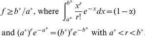
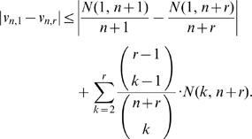
In terms of prediction intervals, if  denotes the
  upper quantile of a standard Normal distribution, it follows from Esty's analysis [23] that if
  is not very near
  or
or  then
then
| (4) |
is approximately a  prediction interval for
  . In practice, and as seen in Fig. 2, when the center of the interval is of a similar or lesser order of magnitude than its radius, the ratio between the upper- and lower-bound of these intervals may oscillate erratically, sometimes over several orders of magnitude. This can be an issue in assessing the depth of sampling in rich environments. For instance, to be highly confident that
  is not of practical use because one may need from
  to
to  additional observations to discover a new species.
Figure 2. Prediction intervals in the human-gut and exponential urn.

95% prediction intervals for the conditional uncovered probability (black) of the human-gut and exponential urn as a function of the number of observations. Esty's prediction intervals in equation (4) (green), and predictions intervals based on the Embedding algorithm (blue, red), using the parameters  and
and  on the left and right, respectively. Blue and red curves correspond to the conservative-lower and -upper prediction intervals for the uncovered probability, respectively. The missing segments on the lower green-curves correspond to Esty's prediction intervals that contained
  . Although the upper- and lower-bound of the Esty's intervals may be of different order of magnitude, our method produces intervals of a constant length in logarithmic scale. This length is controlled by the user-defined parameter
  . In each urn, our method predicted accurately the uncovered probability of a random sub-sample of the
  observations from the urn. See Fig. 4 for the associated rank curve in each urn.
The issues of the aforementioned methods are somewhat expected. On one hand, the problem of predicting  is very different from estimating
  : the former requires predicting the exact proportion of balls in the urn with colors outside the random set
  , rather than in average over all possible such sets. On the other hand, the point estimators of
  are unlikely to predict
  accurately in a logarithmic scale, unless the standard deviation of
  is small relative to
  . Finally, the methods we have described from the literature were designed for static situations i.e. to predict
  or estimate
  when
when  is fixed.
Results
Embedding Algorithm
Here we propose a new methodology to address the issues of the methods presented in the Introduction to predict  . Our methodology lends itself better for a sequential analysis and accurate predictions in a logarithmic scale; in particular, also in a linear scale–though it relies on randomized sample sizes. Due to this, in static situations i.e. for fixed sample sizes, our method only yields predictions for a random sub-sample of the original sample.
Randomized sample sizes are more than just an artifact of our procedure: due to Theorem 1 below, for any predetermined sample size, there is no deterministic algorithm to predict  and
and  unbiasedly, unless the urn is composed by a known and flat distribution of colors. See the Materials and Methods section for the proofs of our theorems.
Theorem 1
If
 is a continuous and one-to-one function then the following two statements are equivalent: (i) there is a non-randomized algorithm based on
 to predict
 conditionally unbiased; (ii) the urn is composed by a known and equidistributed number of colors.
Our methodology is based on a so called Poissonization argument [24]. This technique is often used in allocation problems to remove correlations [25]. It was applied in [26] to show that the cardinality of the random set  is asymptotically Gaussian after the appropriate renormalization. Mao and Lindsay [27] used implicitly a Poissonization argument to argue that intervals such as in equation (4) have a
  asymptotic confidence, under the hypothesis that the times at which each color in the urn is observed obey a homogeneous Poisson point process (HPP) with a random intensity. Here, asymptotic means that the
  -diversity tends to infinity, which entails adding colors into the urn. Our approach, however, is not based on any assumption on the times the data was collected, nor on an asymptotic rescaling of the problem, but rather on the embedding of a sample from an urn into a HPP with intensity
  in the semi-infinite interval
  . We emphasize that the HPP is a mathematical artifice simulated independently from the urn.
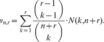
In what follows,  is a user-defined integer parameter. We have implemented the Poissonization argument in what we call the Embedding algorithm in Table 1. For a schematic description of the algorithm see Fig. 3 and, for its heuristic, consult the Materials and Methods section.
Table 1. Embedding algorithm.
| Input: |
 , a set , a set  of colors known to be in the urn, and constants of colors known to be in the urn, and constants  that satisfy condition (5). that satisfy condition (5). |
| Output: | Unbiased predictor of  , ,  prediction interval for prediction interval for  and an updated set and an updated set  of colors known to belong to the urn. of colors known to belong to the urn. |
| Step 1. | Assign  , ,  , and , and  . . |
| Step 2. | While  assign assign  , and sample with replacement a ball from the urn. Let , and sample with replacement a ball from the urn. Let  be the color of the sampled ball. If be the color of the sampled ball. If  then assign then assign  and and  . . |
| Step 3. | Simulate  , and assign , and assign  . . |
| Step 4. | Output  , ,  and and  . . |
Figure 3. Schematic description of the Embedding algorithm.

Suppose that in a first sample from an urn you only observe the colors red, white and blue; in particular,  . Let
. Let  be the unknown proportion in the urn of balls colored with any of these colors i.e.
  . To estimate
  , sample additional balls from the urn until observing
  balls with colors outside
  . Embed the colors of this second sample into a homogeneous Poisson point process with intensity one; in particular, the average separation of consecutive points with colors outside
  are independent exponential random variables with mean
  . The unknown quantity
  can be now estimated from the random variable
  . As a byproduct of our methodology, conditional on
  , if
, if  denotes the relative proportion of color
  in the first sample then
  predicts the true proportion of color
  in the urn.
Suppose that a set  of colors is already known to belong to the urn and let
  be the coverage probability of the colors in this set. We note that, in the context of the previous discussion,
  with
with  .
.
To predict  , draw balls from the urn until
  colors outside
  are observed. Visualize each observation as a colored point in the interval
  . The Poissonization consists in spacing these points out using independent exponential random variables with mean one. Due to the thinning property of Poisson point processes [28], the position
  of the point farthest apart from
  has a Gamma distribution with mean
  . We may exploit this to obtain conditionally unbiased predictors and exact prediction intervals for
  and
and  as follows. Regarding direct predictions of
  , note that measuring
  in a logarithmic rather than linear scale makes more sense when deep sampling is possible.
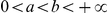
Theorem 2
Conditioned on
 and the event
 , the following applies:
If
 then
then
 is unbiased for
 , with variance
 .
.If
 and
and
 denotes Euler's constant then
 is unbiased for
 , with variance
 , which is bounded between
 and
and
 .
.- If
 ,
,  and
and
 are such that
then the interval
(5)  contains
 with exact probability
 ; in particular,
 contains
 also with probability
 .
.
We note that  is the uniformly minimum variance unbiased estimator of
  based on
  exponential random variables with unknown mean
  . Furthermore,
  converges almost surely to
  , as
, as  tends to infinity; in particular, the point predictors in part (i) and (ii) are strongly consistent.
We also note that the logarithm of the statistic in part (i) under-estimates  in average. In fact, the difference between the natural logarithm of the statistic in (i) and the statistic in (ii) is
  , which is negative for
  , and increases to zero as
  tends to infinity. From a computational stand point, however, the statistics
  and
and  differ by at most
  -units when
  . The same precision may be reached for smaller values of
  if larger bases are utilized. For instance, in base-10, the discrepancy will be at most
  for
for  .
.
In regards to part (iii) of the theorem, we note that our prediction intervals for  cannot contain zero unless
  . On the other hand, since the density function used in equation (5) is unimodal, the shortest prediction interval for
  corresponds to a pair of non-negative constants
  such that:
| (6) |
Similarly, optimal prediction intervals for  follow when
| (7) |
with  (see Materials and Methods for a numerical procedure to approximate these constants). In either case, because
  converges in distribution to a standard Normal as
  tends to infinity, one may select in (5) the approximate constants
 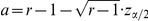 and
and  . With these approximate values, if
  then the true confidence
  of the associated prediction intervals satisfies (see Materials and Methods):
 |
(8) |
(The term on the exponential on the left-hand side above is big-O of  ; in particular, the lower-bound is of the same asymptotic order than the upper-bound.) We note that the constants produced by the Normal approximation may be crude for relatively large values of
  , as seen in Table 2.
Table 2. Optimal versus asymptotic  prediction intervals.

|
Predictioninterval for | Optimalconstants | Gaussianapproximation | Relativeerror 
|

|

|
|
|


|

|

|
|
Same asabove |


|

|

|
|
|


|

|

|
|
Same asabove |


|
As high-throughput technologies allow deeper sampling of microbial communities, it will be increasingly important to have upper- and lower-bounds for  of a comparable order of magnitude. Since the prediction intervals for this quantity in Theorem 2 are of the form
  , and the ratio between the upper- and lower-bound of this interval is
  , one may wish to determine constants
  and
and  such that, not only (5) is satisfied, but also
| (9) |
where  is a user-defined parameter. Not all values of
  are attainable for a given
  and confidence level. In fact, the smallest attainable value is given by the constants associated with the optimal prediction interval for
  . Equivalently,
  is attainable if and only if
 |
Conversely, and as stated in the following result, any value of  is attainable at a given confidence level, provided that the parameter
  is selected sufficiently large.
Theorem 3
Let
 and
and
 be fixed constants. For each
 sufficiently large, there are constants
 such that (5) and (9) are satisfied.
For a given parameter  , there are at most two constants
  such that
  and
and 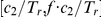 are prediction intervals for
  with exact confidence
  . We refer to these as conservative-lower and conservative-upper prediction intervals, respectively. We refer to intervals of the form
  and
and  as upper- and lower-bound prediction intervals, respectively. See Table 3 for the determination of these constants for various values of
  when
when  .
.
Table 3. Constants associated with 95% prediction intervals.

|

|

|

|

|
| 1 | 2.995732274 |

|

|
0.051293294 |
| 2 | 4.743864518 |

|

|
0.355361510 |
| 3 | 6.295793622 |

|

|
0.817691447 |
| 4 | 7.753656528 | 0.806026244 | 1.360288674 | 1.366318397 |
| 5 | 9.153519027 | 0.924031159 | 1.969902541 | 1.970149568 |
| 6 | 10.51303491 | 1.053998892 | 2.61300725 | 2.613014744 |
| 7 | 11.84239565 | 1.185086999 | 3.28531552 | 3.285315692 |
| 8 | 13.14811380 | 1.315076338 | 3.98082278 | 3.980822786 |
| 9 | 14.43464972 | 1.443547021 | 4.69522754 | 4.695227540 |
| 10 | 15.70521642 | 1.570546801 | 5.42540570 | 5.425405697 |
| 11 | 16.96221924 | 1.696229569 | 6.16900729 | 6.169007289 |
| 12 | 18.20751425 | 1.820753729 | 6.92421252 | 6.924212514 |
| 13 | 19.44256933 | 1.944257623 | 7.68957829 | 7.689578292 |
| 14 | 20.66856908 | 2.066857113 | 8.46393752 | 8.463937522 |
| 15 | 21.88648591 | 2.188648652 | 9.24633050 | 9.246330491 |
| 16 | 23.09712976 | 2.309712994 | 10.03595673 | 10.03595673 |
| 17 | 24.30118368 | 2.430118373 | 10.83214036 | 10.83214036 |
| 18 | 25.49923008 | 2.549923010 | 11.63430451 | 11.63430451 |
| 19 | 26.69177031 | 2.669177032 | 12.44195219 | 12.44195219 |
| 20 | 27.87923964 | 2.787923964 | 13.25465160 | 13.25465160 |
| 21 | 29.06201884 | 2.906201884 | 14.07202475 | 14.07202475 |
| 22 | 30.24044329 | 3.024044329 | 14.89373854 | 14.89373854 |
| 23 | 31.41481021 | 3.141481021 | 15.71949763 | 15.71949763 |
| 24 | 32.58538445 | 3.258538445 | 16.54903872 | 16.54903871 |
| 25 | 33.75240327 | 3.375240328 | 17.38212584 | 17.38212584 |
 upper-bound, conservative-lower, conservative-upper and lower-bound prediction intervals for
  , when
  and
and  . By definition, this means that
 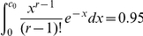 and
and  . Furthermore, the constants
  are solutions to the equation:
 ) denotes that the equation has no solution.
Effect of non-randomized sample sizes
The Embedding algorithm provides conditionally unbiased predictors and intervals for  and
and  , provided that an arbitrary number of additional observations is possible until observing
  balls with colors outside
  . When dealing with fixed sample sizes, there is a positive probability of not meeting this condition, in which case the Embedding Algorithm is inconclusive. In large samples however, such as those collected in microbial datasets, the algorithm may be applied sequentially until it yields an inconclusive prediction. In such case, the true confidence of the prediction intervals produced by the algorithm satisfy the following.
Theorem 4
Suppose that condition (5) is satisfied. Conditioned on
 , if
, if
 balls with colors outside
 are observed in the next
 draws from the urn, then the true confidence
 of the prediction interval for
 produced by the Embedding algorithm satisfies:
if
 then
then
 ;
;if
 then
then
 , where
 is a Gamma random variable with parameters
 , and
, and
 is a Negative Binomial random variable with parameters
 .
.
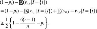
Thus, if the Embedding algorithm produces an output in what remains of a finite sample size, the upper-bound prediction interval for  has at least the user-defined confidence. This is perhaps the case of most interest in applications: it allows the user to estimate the least number of additional samples to observe a color not seen in any sample. For the other three interval types, the true confidence is approximately at least the targeted one if the probability that the algorithm produces an output in what remains of the sample is large.
Discussion
Comparisons with Robbins-Starr estimators
Note that, like Robbins' and Starr's estimators, our method requires extracting additional balls from the urn to make a prediction. However, unlike the methods of the Introduction, our method uses only the additionally collected data–instead of all the data ever collected from the urn–to make a prediction. In terms of sequential analysis, this is advantageous to recover from earlier erroneous predictions (we expand on this point in the next section, see Fig. 1).
In what remains of this section,  hence
hence  , the conditional uncovered probability of a sample of size
  . Furthermore, to rule out trivial cases, we assume that
  with positive probability i.e. the urn is composed by more than just balls of a single color.
Part (i) of Theorem 1 provides a conditionally unbiased predictor for  . We can show, however, that Robbins' and Starr's estimators are not conditionally unbiased for
  in the non-parametric case when
  . To see this argument, first notice that
 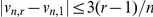 due to the inequality (3). On the other hand, if
  is a color in the urn such that
  then
then
As a result:
 |
Hence, if there exists a color  in the urn that makes the above quantity strictly positive (there are infinitely many such urns, including all urns composed by infinitely many colors, because
  ) then
  cannot be conditionally unbiased for
  .
.
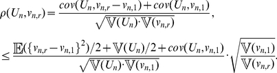
On the other hand, due to parts (i) and (ii) in Theorem 1, we obtain (see Materials and Methods):
 |
(10) |
 |
(11) |
where  denotes correlation and
  variance. Consequently, the point predictors in Theorem 1 are positively correlated with the quantities they were designed to predict. This contrasts with Robbins' estimator, which may be strongly negatively correlated with
  . For instance, if
  for
for  different colors in the urn, it is shown in [21] that the asymptotic correlation between
  and Robbins' estimator
  is asymptotically negative when
  converges to a strictly positive but finite constant
  . In this same regime but provided that
  , we can show that (see Materials and Methods):
| (12) |
Since the right-hand side above is negative for all  sufficiently small, Starr's estimator
  may also have a strong negative correlation with
  when
when  is much smaller than
  .
.
A further calculation based on parts (i) and (ii) in Theorem 1 shows that
In particular, for fixed  , the correlations in equations (10) and (11) approach to one as
  tends to infinity.
Finally, for non-trivial urns with finite  -diversity, i.e. urns composed by balls with at least two but a finite number of different colors, one can show for fixed
  that the correlation in equation (10) approaches
  as
as  tends to infinity. Furthermore, if we again assume that
  for
for  different colors in the urn and
  converges to a strictly positive but finite constant, then the correlation in equation (10) approaches zero from above. As we pointed out before, in this regime, Robbins' estimator is asymptotically negatively correlated with
  .
.
Selection of parameters
There are two main criteria to select the parameter  of the Embedding algorithm in a concrete application.
One criteria applies for point predictors. In this case, conditioned on  , the standard deviation of the relative error of our prediction of
  is
is  (Theorem 2, part (i)). To predict
  ,
,  should be therefore selected as small as possible so as to meet the user's tolerance on the average relative error of our predictions. The same criteria applies for point predictors of
  , for which the standard deviation of the absolute error is of order
  , uniformly for all
  (Theorem 2, part (ii)).
A different criteria applies for prediction intervals. In this case, conditioned on  , the user should first specify the confidence level, and how much larger he wants the upper-prediction-bound to be in relation to the lower-prediction bound of
  . Since the ratio between these last two quantities is given by the parameter
  in (9),
  should be selected as small as possible to meet the user's pre-specified factor
  for the given confidence level of the prediction interval (Theorem 3). See Table 4 for the optimal choice of
  for various values of
  when
when  . Note that for the selected parameter
  , the constants associated with the optimal prediction intervals are given in equations (6) and (7), see Materials and Methods.
Table 4. Optimal selection of parameter  in terms of parameter
  .
.

|

|

|

|
| 80 | 2 | 0.0598276655 | 0.355361510 |
| 48 | 2 | 0.1013728884 | 0.355358676 |
| 40 | 2 | 0.1231379857 | 0.355320458 |
| 24 | 2 | 0.226833483 | 0.346045204 |
| 20 | 3 | 0.320984257 | 0.817610455 |
| 12 | 3 | 0.590243030 | 0.787721610 |
| 10 | 4 | 0.806026244 | 1.360288674 |
| 6 | 6 | 1.822307383 | 2.58658608 |
| 5 | 7 | 2.48303930 | 3.22806682 |
| 3 | 14 | 7.17185045 | 8.27008349 |
| 2.5 | 19 | 11.26109001 | 11.96814857 |
| 1.5 | 94 | 75.9077267 | 76.5492088 |
| 1.25 | 309 | 275.661191 | 275.949782 |
 , when
  ; in particular, for each
  and
and  ,
,  and
and  contain
  with a
  probability. For each
  , the smallest value of
  for which the equation:
Simulations on analytic and non-analytic urns
We tested our methods against an urn with an exponential relative abundance rank curve over  species, and an urn matching the observed distribution of microbes in a human-gut sample from [29]. We also analyzed a sample from a human-hand microbiota found in [30]. The gut and hand data are part of the largest microbial datasets collected thus far (see Fig. 4 for the relative abundance rank curve associated with each urn). The relative abundance rank curve, or for simplicity “rank curve”, associated with an urn is a graphical representation of its composition: the height of the graph above a non-negative integer
  is the fraction of balls in the urn with the
  -th most dominant color.
Figure 4. Rank curves associated with the human-gut, human-hand and exponential urn.

In a rank curve, the relative abundance of a species is plotted against its sorted rank amongst all species, allowing for a quick overview of the evenness of a community. On the left, rank curves associated with the human-gut (blue) and -hand data (green) show a relatively small number of species with an abundance greater than 1%, and a long tail of relatively rare species. The right rank curve of the exponential urn (red) simulates an extreme environment, where relatively excessive sampling is unlikely to exhaust the pool of rare species.
The blue dots and red curves on the plots on the left side in Fig. 1 show very accurate point predictions in log-scale of the conditional uncovered probability (as a function of the number of observations), when we apply the Embedding algorithm to a sample of size  from the human-gut and exponential urn, respectively. In both instances, the parameter
  of the Embedding algorithm was set to
  . The accuracy of our method is confirmed by the red clouds on the plots on the right side of Fig. 1, which are centered around
  . The red clouds also indicate that our predictions recover more easily from offset predictions as compared to Robbins' and Starr's (correlation coefficient of red clouds,
  and
and  on top- and bottom-right, respectively). This is to be expected because the Embedding algorithm relies only on the additionally collected data to make a new prediction, whereas Robbins' and Starr's estimators use all the data ever collected from the urn. On the other hand, the red and blue curves in Fig. 2 show that the conservative-upper and -lower prediction intervals of the conditional uncovered probability (also as a function of the number of observations) contain this quantity with high probability and, unlike Esty's intervals, have a constant length in logarithmic scale. The intervals on the plots on the right side are tighter than those on the left because of the decrease of the parameter
  from
from  to
to  . In each case, the parameter
  was selected according to the guidelines in Table 4. We note that sequential predictions based on the Embedding Algorithm in figures 1 and 2 were produced until the algorithm yielded inconclusive predictions. For this reason, our predictions ended before exhausting each sample.
In the human-hand dataset,  species were observed in a sample of size
  . To simulate draws with replacement from this environment, we produced a random permutation of the data (see Materials and Methods section). Using the Embedding algorithm with parameters
  , and according to our point predictor,
  of the species observed in the sample represent
  of that hand environment; in particular, the remaining
  is composed by at least
  species. Furthermore, according to our upper-bound prediction interval, and with at least a
  confidence, the species not represented in the sample account for less than
  of that environment.
To test the above predictions, we simulated the rare biosphere as follows. We hypothesized that our point prediction of the conditional uncovered probability could be offset by up to one order of magnitude. We also hypothesized that the number of unseen species in the sample had an exponential relative abundance rank curve, composed either by  ,
,  or
or  species. This leads to nine different urns in which to test our methods. These urns are devised such that they gradually change from the almost unchanged urn in the bottom left corner to the urn in the upper right, which is dominated by rare species (see Fig. 5 for the associated rank curves). As seen on the plots in Fig. 6, the Embedding algorithm yields very accurate predictions in each of these nine scenarios, for all the sample sizes considered.
Figure 5. Rank curves associated with the rare biosphere simulation in the human-gut and -hand urn.

Rank curves associated with Fig. 6 (green) and Fig. 7 (blue).
Figure 6. Predictions in the human-hand urn when simulating the rare biosphere.

Prediction of the conditional uncovered probability (black) in nine urns associated with a human-hand urn. Point predictions produced by the Embedding algorithm (blue), point predictions produced by the algorithm each time a new species was discovered (red),  upper-bound interval (orange), and
  conservative-upper interval (green). The algorithm used the parameters
  . The different urns were devised as follows. For each
  (indexing rows) and
  (indexing columns), a mixture of two urns was considered: an urn with the same distribution as the microbes found in a sample from a human-hand and weighted by the factor
  , and an urn consisting of
  colors (disjoint from the hand urn), with an exponentially decaying rank curve and weighted by the factor
  . See Fig. 5 for the rank curve associated with each urn.
As seen in Fig. 7, our predictions are also in excellent agreement with the human-gut dataset when we simulate the rare biosphere. As expected, the conditional uncovered probability almost always lies between the predicted bounds. We also note that the predictions based on the Embedding algorithm are accurate even for a small number of observations. This suggests that our algorithm can be applied to deeply as well as shallowly sampled environments.
Figure 7. Predictions in the human-gut urn when simulating the rare biosphere.

In a sample of size  from a human-gut,
  species were discovered. Based on our methods, we estimate that
  of these species represent
  of that gut environment; hence, the remaining
  is composed by at least
  species. To test our predictions of the conditional uncovered probability (black), we simulated the rare biosphere by adding additional species and hypothesized that our point prediction could be offset by up to one order of magnitude: point predictions produced by the Embedding Algorithm (blue), point predictions produced by the algorithm each time a new species was discovered (red),
  upper-bound (orange), and
  conservative-upper interval (green). The predictions used the parameters
  . The different urns were devised as follows. For each
  (indexing rows) and
  (indexing columns), a mixture of two urns was considered: an urn with the same distribution as the microbes found in the gut dataset, and weighted by the factor
  , and an urn consisting of
  colors (disjoint from the gut urn), with an exponentially decaying rank curve and weighted by the factor
  . See Fig. 5 for the rank curve associated with each urn.
Materials and Methods
Heuristic behind the Embedding algorithm
The number of times a rare color occurs in a sample from an urn is approximately Poisson distributed. In the non-parametric setting, a direct use of this approximation is tricky because “rare” is relative to the sample size and the unknown urn composition. The embedding into a HPP is a way to accommodate for the Poisson approximation heuristic, without making additional assumptions on the urn's composition. To fix ideas, imagine that no ball in the urn is colored black. Make up a second urn with a single ball colored black. We refer to this as the “black-urn”. Now sample (with replacement) balls according to the following scheme: draw a ball from the original- versus black-urn with probability  and
and  , respectively, where
  is a fixed but small parameter. Under this sampling scheme, even the most abundant colors in the original-urn are rare. In particular, the smaller
  is, the closer is the distribution of the number of times a particular set of colors (excluding black) is observed to a Poisson distribution. This approach is not very practical, however, because the number of samples to observe a given number of balls from the original urn can be astronomically large when
  is very small. To overpass this issue imagine drawing a ball every
  -seconds. Draws from the original urn will then be apart
  seconds, where
  has a Geometric distribution with mean
  . As a result:
  , for
, for  . Thus, as
  gets smaller, the time-separations between consecutive samples from the original urn resemble independent Exponential random variables with mean one. The black-urn can therefore be removed from the heuristic altogether by embedding samples from the original urn into a HPP with intensity one over the interval
  .
.
Simulating draws with replacement
To simulate draws with replacement using data already collected from an environment, produce a random permutation of the data. This can be accomplished with low-memory complexity using the discrete inverse transform method to simulate draws–without replacement–from a finite population [31].
Constants associated with optimal prediction intervals
To numerically approximate a pair of constants  such that
  and
and  , where the integer
  and the number
  are given constants, introduce the auxiliary variable
  , and note that the later condition is fulfilled only when
  and
and  . Due to Newton's method, the sequence
  defined recursively as follows converges to the unique
  that satisfies the integrability condition, provided that
  is chosen sufficiently close to
  :
:
Proof of Inequality (3)
First notice that
 |
(13) |
To bound the first term on the right-hand side above, notice that  . As a result, since
 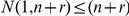 , we obtain that:
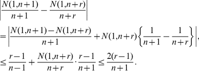 |
(14) |
On the other hand, to bound the second term on the right-hand side of equation (13), define the quantity 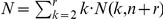 and notice that
  . Using that a weighted average is at most the largest of the terms averaged, we obtain that:
 |
(15) |
where, for the last inequality, we have used that for each  , the associated product is less or equal to the factor associated with the index
  . Equation (3) is now a direct consequence of equations (13), (14) and (15).
Proof of Theorem 1
In what follows,  denotes the inverse function of
  .
.
Define  to be the set of decreasing partitions of
  i.e. vectors of the form
  , with
  and
and  integers, such that
  . To each possible sample
  , let
, let  be the decreasing partition of
  associated with the observed ranks in the sample.
Define  , for each set
  of colors. Part (i) in the theorem is equivalent to the existence of a function
  such that
| (16) |
with probability one. This is because, in the non-parametric setting, the different colors in the urn carry no intrinsic meaning apart from being different. If there is a certain function  which satisfies condition (16) then
  , for each color
  such that
  . In particular, the set
  must be finite. Furthermore, if this set has cardinality
  then
then  , for each color
  in the set; in particular,
  . Condition (ii) is therefore necessary for condition (i). Conversely, if condition (ii) is satisfied and the urn is composed by
  colors occurring in equal proportions then the function
  defined as
  satisfies condition (16).
Proof of Theorem 2
Conditioned on the set  , and the random index
  used in Step 3 of the Embedding algorithm,
  has a Gamma distribution with shape parameter
  and scale parameter
  . However, because
  has a Negative Binomial distribution, conditioned on
  alone,
  has Gamma distribution with shape parameter
  and scale parameter
  . In particular,
  has probability density function
  , for
, for  . From this, parts (i) and (iii) in the theorem are immediate. To show part (ii), notice first that
  is conditionally unbiased for
  , where
The second identity above is due to an integration by parts argument and only holds for  . However, since
  , we obtain that
  , for
, for  . This shows that
  is conditionally unbiased for
  . To complete the proof of the theorem, notice that
  and
and  have the same variance. In particular,
  , where
The last identity above holds only for  . Using that
  , we conclude that
  , for
, for  . As a result:
  ; in particular, since
  ,
,  . The theorem is now a consequence of the following inequalities:
Proof of Equation (8)
Let  and assume that
  . Observe that:
The factor multiplying the previous integral is an increasing function of  ; in particular, due to Stirling's formula, it is bounded by
  from above. Furthermore, from section 6.1.42 in [32], it follows that
On the other hand, if one rewrites the integrand of the previous integral in an exponential-logarithmic form and uses that  , for all
  , where
one sees that
All together, these inequalities imply that
from which the result follows.
Proof of Theorem 3
Due to the Central Limit Theorem, if  and
and  then
then
As a result, for all  sufficiently large,
  , and the integral on the left-hand side above is greater than or equal to
  . Fix any such
  . Since the value of the associated integral may be decreased continuously by increasing the parameter
  , there is
  such that
  and
and
Define  , for
, for  . Since
  and, because
  ,
,  , the continuity of
  implies that there is
  such that
  . Selecting
  and
and  shows the theorem.
Proof of Theorem 4
The proof is based on a coupling argument. First observe that one can define on the same probability space random variables  such that (1)
  and
and  have Negative Binomial distributions with parameters
  , but with
  conditioned to be less than or equal to
  ; (2)
; (2)  but
but  when
when  ; and (3)
  are independent Exponentials with mean
  and independent of
  .
.
Let  be the event “
 balls with colors outside
  are observed in the next
  draws from the urn”. Conditioned on
  , we have that
  and
and  . As a result:
 |
 |
Since  , and because
  when
when  , we obtain that
 |
From this, the upper-bound in part (i) and both inequalities in part (ii) follow after noticing that  has a Gamma distribution with shape parameter
  and scale parameter
  . To show the lower-bound in (i), we again notice that
  . In particular, if
  then
then
 |
Proof of Equations (10) and (11)
Consider random variables  and
and  and a random vector
  , defined on a same probability space. Assume that
  is square-integrable and conditionally unbiassed for
  given
given  i.e.
i.e.  . Furthermore, assume that
  hence
hence  . Because
  is also square-integrable and
  , we obtain that
Hence  .
.
Equation (10) follows by considering  ,
,  and
and  . Similarly, equation (11) follows by considering
 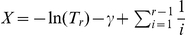 and
and  .
.
Proof of Inequality (12)
First note that
 |
(17) |
Now observe that  because of inequality (13), which implies that
 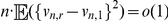 because
  . On the other hand, because Robbins' and Starr's estimators are both unbiased for
  , we have
  . Furthermore, according to the proof of Theorem 2 in [21],
  , therefore
 |
As a result,  . Inequality (12) is now a direct consequence of inequality (17), and the next identities [21]:
Acknowledgments
We would like to thank three anonymous referees for their careful reading of our manuscript and their numerous suggestions, which were incorporated in this final version. The authors are also thankful to R. Knight for contributing to an early version of the code, implementing some of the analyses, and commenting on the manuscript.
Footnotes
Competing Interests: The authors have declared that no competing interests exist.
Funding: M. Lladser was partially supported by NASA ROSES NNX08AP60G and NIH R01 HG004872. R. Gouet was supported by FONDAP, BASAL-CMM and Fondecyt 1090216. J. Reeder was supported by a post-doctoral scholarship from the German Academic Exchange Service (DAAD). M. Lladser and R. Gouet are thankful to the project Núcleo Milenio Información y Aleatoriedad, which facilitated a research visit to collaborate in person. The funders had no role in study design, data collection and analysis, decision to publish, or preparation of the manuscript.
References
- 1.Sogin ML, Morrison HG, Huber JA, Welch DM, Huse SM, et al. Microbial diversity in the deep sea and the underexplored \rare biosphere”. Proc Natl Acad Sci USA. 2006;103:12115–12120. doi: 10.1073/pnas.0605127103. [DOI] [PMC free article] [PubMed] [Google Scholar]
- 2.Hughes JB, Hellmann JJ, Ricketts TH, Bohannan BJ. Counting the uncountable: statistical approaches to estimating microbial diversity. Appl Environ Microbiol. 2001;67:4399–4406. doi: 10.1128/AEM.67.10.4399-4406.2001. [DOI] [PMC free article] [PubMed] [Google Scholar]
- 3.Schloss PD, Handelsman J. Status of the microbial census. Microbiol Mol Biol Rev. 2004;68:686–691. doi: 10.1128/MMBR.68.4.686-691.2004. [DOI] [PMC free article] [PubMed] [Google Scholar]
- 4.Curtis TP, Head IM, Lunn M, Woodcock S, Schloss PD, et al. What is the extent of prokaryotic diversity? Phil Trans R Soc Lond. 2006;361:2023–2037. doi: 10.1098/rstb.2006.1921. [DOI] [PMC free article] [PubMed] [Google Scholar]
- 5.Roesch LF, Fulthorpe RR, Riva A, Casella G, Hadwin AK, et al. Pyrosequencing enumerates and contrasts soil microbial diversity. Isme J. 2007;1:283–290. doi: 10.1038/ismej.2007.53. [DOI] [PMC free article] [PubMed] [Google Scholar]
- 6.Hong SH, Bunge J, Jeon SO, Epstein SS. Predicting microbial species richness. Proc Natl Acad Sci USA. 2006;103:117–122. doi: 10.1073/pnas.0507245102. [DOI] [PMC free article] [PubMed] [Google Scholar]
- 7.Quince C, Curtis TP, Sloan WT. The rational exploration of microbial diversity. Isme J. 2008;2:997–1006. doi: 10.1038/ismej.2008.69. [DOI] [PubMed] [Google Scholar]
- 8.Turnbaugh PJ, Hamady M, Yatsunenko T, Cantarel BL, Duncan A, et al. A core gut microbiome in obese and lean twins. Nature. 2007;457:480–484. doi: 10.1038/nature07540. [DOI] [PMC free article] [PubMed] [Google Scholar]
- 9.Fierer N, Lauber CL, Zhou N, McDonald D, Costello EK, et al. Forensic identification using skin bacterial communities and/or references within. Proc Natl Acad Sci USA. 2010;107:6477–6481. doi: 10.1073/pnas.1000162107. [DOI] [PMC free article] [PubMed] [Google Scholar]
- 10.Magurran AE. Measuring Biological Diversity. Oxford - Blackwell; 2004. [DOI] [PubMed] [Google Scholar]
- 11.Burnham KP, Overton WS. Estimation of the size of a closed population when capture probabilities vary among animals. Biometrika. 1978;65:625–633. [Google Scholar]
- 12.Chao A. Nonparametric estimation of the number of classes in a population. Scand J Stat. 1984;11:265–270. [Google Scholar]
- 13.Chao A. Estimating the population size for capture-recapture data with unequal catchability. Biometrics. 1897;43:783–791. [PubMed] [Google Scholar]
- 14.Mao CX, Lindsay BG. Estimating the number of classes. Ann Stat. 2007;35:917–930. [Google Scholar]
- 15.Bunge J, Fitzpatrick M. Estimating the number of species: A review. J Am Stat Assoc. 1993;88:364–373. [Google Scholar]
- 16.Hinsley F, Stripp A. Codebreakers: The Inside Story of Bletchley Park. Oxford Univ. Press; 1993. [Google Scholar]
- 17.Finch SJ, Mendell NR, Thode HC., Jr Probabilistic measures of adequacy of a numerical search for a global maximum. J Am Stat Assoc. 1989;84:1020–1023. [Google Scholar]
- 18.Mao CX. Predicting the conditional probability of discovering a new class. J Am Stat Assoc. 2004;99:1108–1118. [Google Scholar]
- 19.Good IJ. The population frequencies of species and the estimation of population parameters. Biometrika. 1953;40:237–264. [Google Scholar]
- 20.Robbins HE. On estimating the total probability of the unobserved outcomes of an experiment. Ann Math Stat. 1968;39:256–257. [Google Scholar]
- 21.Starr N. Linear estimation of the probability of discovering a new species. Ann Stat. 1979;7:644–652. [Google Scholar]
- 22.Clayton MK, Frees EW. Nonparametric estimation of the probability of discovering a new species. J Am Stat Assoc. 1987;82:305–311. [Google Scholar]
- 23.Esty WW. A Normal limit law for a nonparametric estimator of the coverage of a random sample. Ann Statist. 1983;11:905–912. [Google Scholar]
- 24.Aldous D. Probability Approximations via the Poisson Clumping Heuristic. Springer-Verlag; 1988. [Google Scholar]
- 25.Mahmoud HM. Sorting: A Distribution Theory. Wiley-Interscience; 2000. [Google Scholar]
- 26.Hwang HK, Janson S. Local limit theorems for finite and infinite urn models. Ann Probab. 2008;36:992–1022. [Google Scholar]
- 27.Mao CX, Lindsay BG. A poisson model for the coverage problem with a genomic application. Biometrika. 2002;89:669–681. [Google Scholar]
- 28.Durrett R. Essentials of stochastic processes. Springer Texts in Statistics; 1999. [Google Scholar]
- 29.Turnbaugh PJ, Ridaura VK, Faith JJ, Rey FE, Knight R, et al. The e_ect of diet on the human gut microbiome: A metagenomic analysis in humanized gnotobiotic mice. Sci Transl Med. 2009;1:6ra14. doi: 10.1126/scitranslmed.3000322. [DOI] [PMC free article] [PubMed] [Google Scholar]
- 30.Fierer N, Hamady M, Lauber CL, Knight R. The influence of sex, handedness, and washing on the diversity of hand surface bacteria. Proc Natl Acad Sci USA. 2008;105:17994–17999. doi: 10.1073/pnas.0807920105. [DOI] [PMC free article] [PubMed] [Google Scholar]
- 31.Ross SM. Simulation. Academic Press, third edition; 2002. [Google Scholar]
- 32.Abramowitz M, Stegun IA. Handbook of Mathematical Functions with Formulas, Graphs, and Mathematical Tables. New York: Dover, ninth Dover printing, tenth GPO printing edition; 1964. [Google Scholar]