

Abstract
Inferring population structure using Bayesian clustering programs often requires a priori specification of the number of subpopulations,  , from which the sample has been drawn. Here, we explore the utility of a common Bayesian model selection criterion, the Deviance Information Criterion (DIC), for estimating
  . We evaluate the accuracy of DIC, as well as other popular approaches, on datasets generated by coalescent simulations under various demographic scenarios. We find that DIC outperforms competing methods in many genetic contexts, validating its application in assessing population structure.
Introduction
A common problem in modern population genetics is identifying population substructure among a sample of individuals genotyped across a set of neutral genetic markers. Bayesian clustering algorithms such as STRUCTURE [1], [2] and BAPS [3] and their derivates [4]–[8] are commonly used for addressing this problem. Of particular concern to many investigators is estimating the number of subpopulations or clusters  that are necessary and sufficient to explain observed patterns of genetic variation. Part of the reason investigators are concerned with the “choosing
  ” problem is that many of the classification algorithms (including STRUCTURE) require specifying the number of clusters as a parameter in the model. A consequence of this is that the biological conclusions one draws from the data may be artificially dependent on the value of
  chosen. In practice, many investigators analyze their data using a range of values for
  , reporting the output for all (or a plausible set of)
  's and/or employ one of several post hoc statistics [1], [4], [9] to choose an optimal value for
  . The purpose of this communication is to report our experience with the Deviance Information Criterion (DIC) as a statistic for choosing
  . By comparing the performance of DIC to other commonly used statistics on simulated data under a variety of population genetic scenarios, we find that it often outperforms other approaches and recommend it be considered by investigators interested in estimating
  from genotype data. Its advantage over more complex approaches such as the reversible-jump Markov chain Monte Carlo (MCMC) or the Dirichlet process prior on
  , is that calculating DIC requires trivial computational overhead once the MCMC has been run.
Choosing  is a difficult problem in the Bayesian clustering setting, because as
  increases, the likelihood of the data increases monotonically, as well as the complexity of the model. Adding more degrees of freedom to the analysis generally improves the overall fit of the model to data. This often results in monotonic non-decrease in the probability of the data given
  as
as  increases [1], [9]. A common way of dealing with this class of statistical problems (known as “model selection”) is to use a penalizing function which weighs the fit of a model versus its complexity. This is the underlying idea behind many model selection statistics such as the Akaike Information Criterion (AIC) and the Bayesian Information Criterion (BIC). The Deviance Information Criterion (DIC) is a recently proposed statistic for model selection when the posterior distribution of parameters in competing models are estimated using Markov chain Monte Carlo, as is the case with STRUCTURE and its derivatives [10].
Results
We applied the Deviance Information Criterion to estimate  for datasets generated by coalescent simulations under various demographic scenarios and for the large-scale genotype data from Human Genome Diversity Panel. We evaluated the accuracy of DIC in comparison with other popular approaches and demonstrate that DIC performs well in a variety of scenarios.
Application to Simulated Data
We performed extensive coalescent simulations using multiple demographic models, including Models Split, Tree,  ,
,  ,
,  and Inbred (see Section Methods and Figure 1). Models Split and Tree implement the distinct demographic histories during subpopulation formation. Models
  ,
,  , and
, and  are used to investigate the impact of different levels of exchange among subpopulations on the inference of population structure. Model Inbred is designed to test the effect of the confounding factor “inbreeding”. To evaluate the robustness of our method in the case of scarcity of data, we also simulate the Model Split with
  individuals or
  SNPs. The last scenario tested is to reduce the splitting time among subpopulations by a factor of ten. This is equivalent to decreasing the genetic distances among subpopulations, which implicitly reflects the various levels of physical distances among populations. Then we ran each data set through InStruct [5] with five MCMC chains for each value of
  , retaining a total of 50,000 iterations after a 500,000 iteration burn-in period with a thinning interval of ten iterations between retained draws. Figure 2 illustrates the performance of DIC on a randomly selected data set generated under Model Split with true
  . For these four data sets,
  always peaked at the correct
  values for all the chains. (Note that we choose to plot
  because it is often easier to visualize a maximum peak than a minimum trough).
Figure 1. Subpopulation topology of Model Split and Model Tree for ranging from three to five.

In Model Split, subpopulations are split from one ancestral population simultaneously, forming a star-shaped topology. In Model Tree, populations separate at different time points, forming a tree-shaped topology. The time interval between two consecutive dashed lines is 0.5 scaled in units of  generations, where
  is the effective population size.
Figure 2. Performance of DIC on one data set simulated under Model Split for each true  value, 1,2,3 and 5.

To place our work in a broader context, we also ran these data sets through five methods commonly used to estimate  : (1) the approximate likelihood method implemented in STRUCTURE using both the original and correlated allele frequency model, (i.e., the “F” model [1], [2]), (2) the
  approach based on running STRUCTURE with both the original and F models [9], (3) Eigenanalysis method (implemented in “SmartPCA” software) proposed by Patterson et al. [11] which estimates
  as 1 plus the number of significant eigenvalues underlying a principal component decomposition (PCD) of the scaled genotypic value matrix, (4) Structurama which uses a Dirichlet process prior model to partition a sample into subgroups [12], [13], and (5) BAPS utilizing the splitting and merging strategy to attain the best classification [3], [6]–[8]. We also conducted preliminary analyses using the regularization method [4], but found that it consistently performed poorly for moderate values of
  (e.g., the accuracy was under 50% when
  under the Split model).
We assessed the accuracy of each method as the proportion of data sets which correctly recover the value of  used in data simulation using the optimality criterion defined for each approach. For example, for DIC, we used the lowest DIC value observed across five independent MCMC chains run for each of the six values of
  . For Eigenanalysis, we assessed accuracy under three significance levels (
 and
and  ). For Structurama, we chose the partitions of individuals with the highest posterior probabilities under two prior distributions: (1) a noninformative prior on the number of clusters, and (2) a prior distribution with the expected number of clusters equal to the true value of
  used to simulate the data. We use the individual clustering mode of BAPS as our simulation does not include admixture.
Under the case of simple population splitting with a high degree of population differentiation, i.e.,  values around
  , we found that the DIC method consistently outperformed other approaches (see Table 1). For example, under Model Split, the accuracy is near 100% for all values of
  considered. STRUCTURE, on the other hand, has an accuracy that ranges from 54% to 100% depending on the true
  and whether or not the
  model is employed. We also observe that the accuracy of
  decays with
  , starting at 100% for
  and reaching
  and
and  for the
  and non-
 models, respectively, at
  . Eigenanalysis tends to perform well, but is sensitive to the choice of
  with smaller values (e.g.,
  ) of
) of  performing better than higher values (e.g.,
  ). The performance of Structurama on simulated data was interesting. It performed perfectly well when
  was small (
 ) but when
  , it tended to fail almost completely. We posit that this may be due to the tendency of the Dirichlet process mixture model to overcluster, which results in
  being underestimated. An alternative explanation is that the Dirichlet process prior fails to converge within a finite number of iterations in practice, which commonly challenges many other mixture model methods [14]. BAPS performs perfectly well, except in the case of
  , it drops to 82%. The performance of most methods under the complex splitting model (i.e., Model Tree) was similar to the performance under Model Split. This implies our results are robust to moderate deviations from the
  -wise subpopulation split topology assumed in STRUCTURE.
Table 1. Accuracy of multiple  estimators under Models Split and Tree.
| Model | Split | Tree | ||||||
| K | 1 | 2 | 3 | 4 | 5 | 3 | 4 | 5 |

|
0.495 | 0.502 | 0.493 | 0.492 | 0.486 | 0.507 | 0.501 | |
| DIC | 1.00 | 1.00 | 1.00 | 1.00 | 1.00 | 1.00 | 1.00 | 0.98 |
| STRUCTURE | 0.90 | 1.00 | 1.00 | 0.86 | 0.80 | 0.98 | 0.94 | 0.72 |
| STRUCTURE, F model | 0.90 | 0.98 | 0.94 | 0.82 | 0.54 | 0.90 | 0.82 | 0.62 |

|
1.00 | 0.94 | 0.70 | 0.64 | 0.80 | 0.86 | 0.64 | |
 , F model , F model |
1.00 | 0.90 | 0.78 | 0.50 | 0.84 | 0.92 | 0.54 | |
Eigenanalysis, 
|
0.97 | 0.89 | 0.86 | 0.86 | 0.96 | 0.96 | 0.92 | 0.90 |
Eigenanalysis, 
|
1.00 | 0.96 | 0.91 | 0.93 | 0.99 | 0.98 | 0.94 | 0.92 |
Eigenanalysis, 
|
1.00 | 1.00 | 0.96 | 0.96 | 1.00 | 1.00 | 0.96 | 0.96 |
| Structurama, noninformative prior | 1.00 | 1.00 | 0.82 | 0.18 | 0.02 | 0.88 | 0.22 | 0.00 |
| Structurama, correct prior | 1.00 | 1.00 | 0.82 | 0.18 | 0.02 | 0.82 | 0.22 | 0.00 |
| BAPS | 1.00 | 1.00 | 1.00 | 0.82 | 1.00 | 1.00 | 1.00 | 0.96 |
Performance assessment of methods including DIC, STRUCTURE,  , Eigenanalysis, Structurama and BAPS. “
 ” is the population differentiation statistic estimated by SmartPCA [11] averaged across 50 data sets. STRUCTURE's performance is evaluated based upon both the original model and the correlated alleles or “F” model. Similarly tested is the
  statistic that relies on STRUCTURE. Eigenanalysis is tested at three significance levels (
 ). Structurama is assessed using both a noninformative prior on
  and the true
  value as the starting point. BAPS is evaluated using the individual clustering mode. Blank values in the table indicate that a program did not generate a result.
Migration among subpopulations, on the other hand, can have a profound impact on the accuracy of all approaches. When migration rates are low between subpopulations (Model  ), DIC, BAPS, and Eigenanalysis with a stringent p-value cutoff both worked perfectly. STRUCTURE also performed reasonably well with accuracy rates ranging between 84% and 100% (see Table 2). When the migration rates among subpopulations are intermediate (
 corresponding to
  ), most methods showed results similar to those under Model
  . The notable exception was Structurama which performed poorly (at least under the parameter values we explored). Under low population differentiation (
 ;
;  ), all methods showed a decrease in accuracy. For example, the accuracy of DIC noticeably decreases with
  reaching a low of
  for
for  (see Table 3). The original STRUCTURE model also performed poorly with accuracy well below
  . Interestingly, in the case of strong migration, the
  model's accuracy is much higher both for the STRUCTURE and
  statistics. This is probably because the correlated alleles model is doing a good job in modeling patterns of genetic variation among admixed subpopulations. Since InStruct does not implement an
  model, we predict that adding the
  model to InStruct or implementing DIC within STRUCTURE with the
  model would perform as well or better than these statistics. Eigenanalysis also seems to handle the high migration rate scenario well. Its accuracy decreases only slightly with
  , compared to the low migration rate case. Intriguingly, the most stringent significance level for high migration does not necessarily perform best, as it does with the slower migration models. This suggests that it may be challenging to find the optimal tuning of
  for best classification accuracy when using PCD and a Tracy-Widom approximation to the distribution of p-values. We also observe that Structurama appears to be very sensitive to migration. It clusters all individuals into one group for every data set under Model
  , i.e. no matter which prior is used, Structurama incorrectly estimates
  for every simulated data set. Our results differ from [12], who found Structurama worked well in estimating
  under certain scenarios. We believe the differences may be due to the details of the simulation used. They considered an island model with migration, whereas we used a population-split model with subsequent migration among demes. This slight difference leads to more subpopulation differentiation in their simulations than ours, since they have a longer expected coalescent time between demes than we do. (That is, in our simulations all demes merge, looking back in time, at the time of population splitting). BAPS's accuracy decreases sharply as
  increases, implying that it performs poorly in the case of weak population differentiation.
Table 2. Accuracy of multiple  estimators under Models
  and
and  .
.
| Model |
 , slow migration , slow migration |
 , moderate migration , moderate migration |
||||||
| K | 2 | 3 | 4 | 5 | 2 | 3 | 4 | 5 |

|
0.392 | 0.430 | 0.452 | 0.454 | 0.191 | 0.248 | 0.263 | 0.281 |
| DIC | 1.00 | 1.00 | 1.00 | 1.00 | 1.00 | 1.00 | 1.00 | 1.00 |
| STRUCTURE | 1.00 | 0.98 | 0.94 | 0.84 | 1.00 | 1.00 | 0.96 | 0.84 |
| STRUCTURE, F model | 0.88 | 0.96 | 0.94 | 0.88 | 0.86 | 0.86 | 0.94 | 0.86 |

|
1.00 | 0.78 | 0.94 | 0.80 | 1.00 | 0.92 | 0.76 | 0.80 |
 , F model , F model |
1.00 | 0.84 | 0.94 | 0.88 | 1.00 | 0.96 | 0.80 | 0.92 |
Eigenanalysis, 
|
0.96 | 0.84 | 0.98 | 0.96 | 1.00 | 0.86 | 0.94 | 0.98 |
Eigenanalysis, 
|
0.98 | 0.94 | 1.00 | 0.96 | 1.00 | 0.98 | 0.98 | 1.00 |
Eigenanalysis, 
|
0.98 | 1.00 | 1.00 | 1.00 | 1.00 | 1.00 | 1.00 | 1.00 |
| Structurama, noninformative prior | 1.00 | 0.96 | 0.80 | 0.44 | 0.74 | 0.52 | 0.12 | 0.00 |
| Structurama, correct prior | 1.00 | 0.98 | 0.78 | 0.44 | 0.72 | 0.52 | 0.10 | 0.06 |
| BAPS | 1.00 | 1.00 | 1.00 | 1.00 | 1.00 | 1.00 | 1.00 | 0.98 |
Evaluation of these methods are performed in the same manner as in Table 1.
Table 3. Accuracy of multiple  estimators under Models
  and Inbred.
| Model |
 , fast migration , fast migration |
Inbred | |||||||
| K | 2 | 3 | 4 | 5 | 1 | 2 | 3 | 4 | 5 |

|
0.048 | 0.063 | 0.069 | 0.073 | 0.489 | 0.498 | 0.491 | 0.504 | |
| DIC | 1.00 | 0.94 | 0.70 | 0.56 | 1.00 | 1.00 | 1.00 | 0.98 | 0.98 |
| STRUCTURE | 0.02 | 0.02 | 0.06 | 0.16 | 0.64 | 1.00 | 0.98 | 0.90 | 0.84 |
| STRUCTURE, F model | 0.90 | 0.98 | 1.00 | 1.00 | 0.34 | 0.36 | 0.22 | 0.20 | 0.22 |

|
0.32 | 0.48 | 0.26 | 0.16 | 1.00 | 0.74 | 0.80 | 0.68 | |
 , F model , F model |
0.94 | 0.96 | 0.74 | 0.64 | 1.00 | 0.94 | 0.84 | 0.82 | |
Eigenanalysis, 
|
0.94 | 0.96 | 0.90 | 0.94 | 0.86 | 0.68 | 0.61 | 0.66 | 0.68 |
Eigenanalysis, 
|
1.00 | 0.98 | 0.90 | 0.90 | 0.96 | 0.92 | 0.73 | 0.78 | 0.75 |
Eigenanalysis, 
|
1.00 | 0.92 | 0.90 | 0.84 | 1.00 | 0.93 | 0.81 | 0.84 | 0.85 |
| Structurama, noninformative prior | 0.00 | 0.00 | 0.00 | 0.00 | 1.00 | 1.00 | 0.82 | 0.24 | 0.02 |
| Structurama, correct prior | 0.00 | 0.00 | 0.00 | 0.00 | 1.00 | 1.00 | 0.78 | 0.22 | 0.02 |
| BAPS | 0.64 | 0.54 | 0.22 | 0.14 | 0.74 | 1.00 | 1.00 | 1.00 | 0.98 |
Evaluation of these methods are performed in the same manner as in Table 1.
When we assessed accuracy under the inbreeding model, assuming undetected inbreeding (such as partial self-fertilization) within subpopulations, we found again that DIC tends to outperform other methods (see Table 3). It is important to note that in calculating DIC, we have used InStruct's inbreeding model whereas the other approaches based on STRUCTURE assume the Hardy-Weinberg equilibrium within clusters. We, and others, have shown that failing to consider inbreeding in the likelihood calculation for STRUCTURE can lead to spurious signals of population admixture and erroneous inference of the number of subpopulations [5]. This phenomenon appears to cause a large reduction in the accuracy of estimating  by STRUCTURE's
  model with only 20% of simulations uncovering the true number of populations underlying the data. Eigenanalysis, which does not account for inbreeding either, likewise overestimates the number of subpopulations, and has an accuracy ranging from
  to
to  depending on the true value of
  . Both Structurama and BAPS are not heavily affected by hidden inbreeding, and have the similar accuracy pattern as under Model Split.
To assess the robustness of DIC in the limit of small data sets, we simulated data under Model Split for  individuals or
  SNPs. We found that the accuracy of DIC is robust to the former, but not the latter (Table 4). When the subpopulation size decreases to 10, DIC performs almost as well as with a larger number of individuals per subpopulation. STRUCTURE and
  , on the other hand, show a significant reduction in accuracy as
  increases to 5. Eigenanalysis shows a reduction in accuracy only when using a stringent p-value cutoff. When the number of markers is reduced to only 10, DIC's accuracy falls to 42% when
  increases to five, which is expected as DIC is an asymptotic approximation that only holds as the sample size is sufficiently large, and the accuracy of STRUCTURE and
  is close to zero. With so few markers, Eigenanalysis fails to provide an output. Structurama also performs poorly under larger values of
  s. BAPS is robust to the decrease in sample size but is strongly affected by reducing the number of markers. While we conclude that DIC is more robust than other approaches to small data sizes, we, of course, expect accuracy to increase with
  and so recommend that investigators genotype as many unlinked markers as is economically feasible.
Table 4. Accuracy of multiple  estimators with reduced data dimensions.
| Model | Subpopulation Size = 10 | Number of Loci = 10 | ||||||||
| K | 1 | 2 | 3 | 4 | 5 | 1 | 2 | 3 | 4 | 5 |
| DIC | 1.00 | 1.00 | 1.00 | 1.00 | 0.98 | 1.00 | 1.00 | 0.82 | 0.42 | 0.48 |
| STRUCTURE | 0.84 | 1.00 | 0.86 | 0.60 | 0.40 | 1.00 | 0.96 | 0.86 | 0.72 | 0.18 |
| STRUCTURE, F model | 0.16 | 1.00 | 0.86 | 0.66 | 0.34 | 0.10 | 0.96 | 0.86 | 0.72 | 0.18 |

|
0.98 | 0.68 | 0.64 | 0.22 | 0.94 | 0.24 | 0.06 | 0.04 | ||
 , F model , F model |
0.98 | 0.86 | 0.62 | 0.16 | 0.94 | 0.20 | 0.10 | 0.04 | ||
Eigenanalysis, 
|
0.90 | 0.80 | 0.82 | 0.80 | ||||||
Eigenanalysis, 
|
0.96 | 0.84 | 0.88 | 0.92 | ||||||
Eigenanalysis, 
|
0.20 | 0.42 | 0.66 | 0.78 | ||||||
| Structurama, noninformative prior | 1.00 | 1.00 | 0.96 | 0.38 | 0.00 | 1.00 | 0.90 | 0.40 | 0.14 | 0.00 |
| Structurama, correct prior | 1.00 | 1.00 | 0.96 | 0.38 | 0.00 | 1.00 | 0.90 | 0.38 | 0.12 | 0.00 |
| BAPS | 1.00 | 1.00 | 1.00 | 0.8 | 0.5 | 0.00 | 0.02 | 0.04 | 0.36 | 0.28 |
Evaluation of these methods are performed in the same manner as in Table 1. Data are simulated under Model Split with the size of each subpopulation reduced from 50 to 10 and the number of loci reduced from 100 to 10, respectively.
Under the Split model, our simulated data sets had a high degree of population differentiation ( among clusters was around
  ). To investigate the effect of weaker population structure on estimation accuracy, we simulated data with a reduced splitting time of 0.05 in units of
  generations. This gives simulated data with
  among subpopulations in the range of
  . We found that shortening the splitting time, not surprisingly, reduced the accuracy of all methods with results similar to those observed for the strong migration among subpopulations (Model
  ). We note, in particular, that the Bayesian methods showed a decrease in accuracy with increasing
  . Interestingly, Eigenanalysis performed quite well, particularly using the less stringent significance level (see Table 5), which is consistent with the original results of [11] that their approach can detect very fine-scale population structure.
Table 5. Accuracy of multiple  estimators with shorter splitting time among subpopulations.
| Model | Subpopulation Splitting Time = 0.05 | ||||
| K | 1 | 2 | 3 | 4 | 5 |

|
0.090 | 0.084 | 0.093 | 0.097 | |
| DIC | 1.00 | 1.00 | 0.92 | 0.60 | 0.26 |
| STRUCTURE | 0.64 | 0.78 | 0.50 | 0.54 | 0.22 |
| STRUCTURE, F model | 0.76 | 1.00 | 0.94 | 0.94 | 0.74 |

|
1.00 | 0.44 | 0.08 | 0.04 | |
 , F model , F model |
0.96 | 0.78 | 0.56 | 0.42 | |
Eigenanalysis, 
|
0.96 | 0.96 | 0.94 | 0.9 | 0.72 |
Eigenanalysis, 
|
1.00 | 1.00 | 0.98 | 0.94 | 0.70 |
Eigenanalysis, 
|
1.00 | 1.00 | 0.98 | 0.88 | 0.48 |
| Structurama, noninformative prior | 1.00 | 0.00 | 0.00 | 0.00 | 0.00 |
| Structurama, correct prior | 1.00 | 0.00 | 0.00 | 0.00 | 0.00 |
| BAPS | 1.00 | 1.00 | 0.58 | 0.02 | 0.00 |
Evaluation of these methods are performed in the same manner as in Table 1. Data are simulated under Model Split with the splitting time reduced from  to
to  .
.
Application to Human Data
To demonstrate a concrete application of DIC, we have applied the approach with the inbreeding model of InStruct to the Human Genome Diversity Panel (HGDP-CEPH) data from [15], containing 1056 individuals from 52 populations, genotyped at 377 autosomal microsatellite loci. We find that DIC estimates  for these data as shown in Figure 3A. The five clusters we estimate (see Figure 3B) correspond approximately to the geographic regions of Africa, Europe/the Middle East/Central-South Asia, the Americas, East Asia, and Oceania as described by [15]. It is interesting to note that in our classification, we also found evidence that some alleles from the San people of Namibia, Africa, may form a sixth minor cluster with a posterior inbreeding coefficient estimate around 0.20, the highest of all clusters.
Figure 3. Analysis result of data from the Human Genome Diversity Panel.

A. Estimated DIC for different values of  . B. Distruct classification bar plot of individuals from the above data set assuming
  . Each vertical bar represents one individual and each color represents a different cluster.
Discussion
The Deviance Information Criterion is a simple and effective model selection method for estimating  , the number of clusters underlying a sample of individuals. We anticipate this approach will have wide applications in population structure inference. One important factor affecting our estimation of the accuracy of DIC is the underlying probabilistic model used in InStruct. Since InStruct takes inbreeding into account, it naturally outperforms approaches that do not model non-random mating explicitly. At the same time, since we do not implement the
  model, we do poorly when migration rates are high and allele frequencies are similar among clusters. Furthermore, the accuracy of DIC sometimes fluctuates with the quality of the classification of individuals into clusters. As in any complex MCMC framework, the likelihood surface may be multimodal for a given value of
  . In practice, we have observed that DIC values may vary substantially among independent MCMC chains for the same dataset, especially for larger
  values, due to poor mixing of MCMCs under some scenarios. We recommend that for a given value of
  , several chains be run and the minimum value of DIC across chains be used for inference. It is also important to note that population structure is a complex concept with a hierarchical form and multiple levels. DIC infers the best partition of a group of individual genetic materials taken as a whole. To investigate the finer scale of subpopulation structure, we suggest further structure analysis within each inferred cluster.
Methods
DIC Statistic
Here we introduce the Deviance Information Criterion formula in details. Denote  for
for  as the probability of observing individual
  's genotype given parameters
  of the model which include factors such as subpopulation allele frequencies, probabilities of assignment, inbreeding coefficients, etc. For a given multivariate parameter vector
  , we define the deviance as:
The above formula is easily recognized as the usual log-likelihood function evaluated at  . [10] defines the Deviance Information Criterion as
where  is the posterior mean deviance and
  is a point estimate of the parameters. The quantity
  is an estimate of the “effective number of parameters in the model”. We estimate
  using
using  retained Markov chain Monte Carlo draws:
where  represent the retained values of the parameters at iteration
  . In the Bayesian clustering problem, point estimates of
  can often be ill-behaved due to the label-switching problem, and according to [16], a more stable estimator of DIC for mixture models is based on averaging the likelihood over retained draws:
where
is the average value of the likelihood function for individual  across retained draws from an MCMC chain. As with AIC and BIC, a smaller value of DIC indicates a better fitting model. We implemented the Deviance Information Criterion in our program InStruct [5] accessible through the web interface http://cbsuapps.tc.cornell.edu/InStruct.aspx.
Data Simulation
To demonstrate the performance of DIC and compare it with other methods, we used the standard coalescent simulation program “ms” [17] to generate data under various genetic scenarios. For each population substructure scenario, we assumed a sample of  subpopulations for
  , and equal and constant subpopulation sizes of 50 individuals genotyped at 100 unlinked neutral diallelic (i.e., SNP) loci. Six major genetic contexts considered in our simulation are listed below:
Model Split  subpopulations that split without subsequent migration.
Model Tree  subpopulations with a tree-shaped relationship describing the splitting process.
Model
M0.5
 subpopulations with a scaled migration rate
 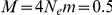 between any of two subpopulations.
Model
M2.0
 subpopulations with a scaled migration rate
  between any of two subpopulations.
Model
M10
 subpopulations with a scaled migration rate
  between any of two subpopulations.
Model Inbred  subpopulations without migration, each subpopulation with a randomly sampled selfing rate.
For Model Split,  ,
,  ,
,  and Inbred, all subpopulations split from a common ancestral population at a time
  in the past scaled in units of
  generations, where
  is the effective subpopulation size. In Model Inbred, partial self-fertilization within subpopulations is taken into account using the same simulation scheme as in [5]. For Models
  ,
,  and
and  ,
,  is omitted as there is no migration in the case of only one subpopulation. Besides the star-shaped genealogy among subpopulations in Model Split, Inbred,
  ,
,  and
and  , we also considered the tree topology relationship among subpopulations described in Model Tree as illustrated in Figure 1. For this model, the
  and
and  cases are ignored since they are identical to the corresponding
  s under Model Split.
To assess the robustness of our conclusions to changes in sample size, the number of loci genotyped, or population divergence time, we undertook further simulations using Model Split. First, we reduced subpopulation size from  to
to  . Second, we reduced the number of markers used in the analysis from 100 to 10. Third, we reduced the splitting time from the common ancestral population from
  to
to  . For each of the nine contexts described above (6 models+3 robustness conditions), we simulated 50 replicate data sets per value of
  .
.
Acknowledgments
We appreciate many thoughtful comments from Rasmus Nielsen and Nick Patterson on the manuscript. We also thank Nick Patterson for the suggestion of using SmartPCA to estimate FST.
Footnotes
Competing Interests: The authors have declared that no competing interests exist.
Funding: This work is funded by National Science Foundation Grant #0606461 to Susan McCouch, Carlos D. Bustamante, Georgia Eizenga and Anna McClung. The work of running the software BAPS by Dr. Yidong Lei is funded by the National Natural Science Foundation of China (Grant #40771084). The funders had no role in study design, data collection and analysis, decision to publish, or preparation of the manuscript.
References
- 1.Pritchard JK, Stephens M, Donnelly P. Inference of population structure using multilocus genotype data. Genetics. 2000;155:945–59. doi: 10.1093/genetics/155.2.945. [DOI] [PMC free article] [PubMed] [Google Scholar]
- 2.Falush D, Stephens M, Pritchard JK. Inference of population structure using multilocus genotype data: linked loci and correlated allele frequencies. Genetics. 2003;164:1567–87. doi: 10.1093/genetics/164.4.1567. [DOI] [PMC free article] [PubMed] [Google Scholar]
- 3.Corander J, Waldmann P, Sillanpaa M. Bayesian analysis of genetic differentiation between populations. Genetics. 2003;163:367–74. doi: 10.1093/genetics/163.1.367. [DOI] [PMC free article] [PubMed] [Google Scholar]
- 4.Francois O, Ancelet S, Guillot G. Bayesian clustering using hidden markov random fields in spatial population genetics. Genetics. 2006;174:805–16. doi: 10.1534/genetics.106.059923. [DOI] [PMC free article] [PubMed] [Google Scholar]
- 5.Gao H, Williamson S, Bustamante CD. An mcmc approach for joint inference of population structure and inbreeding rates from multi-locus genotype data. Genetics. 2007;176:1635–51. doi: 10.1534/genetics.107.072371. [DOI] [PMC free article] [PubMed] [Google Scholar]
- 6.Corander J, Waldmann P, Marttinen P, Sillanpää M. Baps 2: enhanced possibilities for the analysis of genetic population structure. Bioinformatics. 2004;20:2363–2369. doi: 10.1093/bioinformatics/bth250. [DOI] [PubMed] [Google Scholar]
- 7.Corander J, Marttinen P. Bayesian identification of admixture events using multi-locus molecular markers. Molecular Ecology. 2006;15:2833–2843. doi: 10.1111/j.1365-294X.2006.02994.x. [DOI] [PubMed] [Google Scholar]
- 8.Corander J, Tang J. Bayesian analysis of population structure based on linked molecular information. Mathematical Biosciences. 2007;205:19–31. doi: 10.1016/j.mbs.2006.09.015. [DOI] [PubMed] [Google Scholar]
- 9.Evanno G, Regnaut S, Goudet J. Detecting the number of clusters of individuals using the software structure: a simulation study. Molecular Ecology. 2005;14:2611–2620. doi: 10.1111/j.1365-294X.2005.02553.x. [DOI] [PubMed] [Google Scholar]
- 10.Spiegelhalter DJ, Best NG, Carlin BP, van der Linde A. Bayesian measures of model complexity and fit. Journal of Royal Statistical Society, Series B. 2002;64:538–640. [Google Scholar]
- 11.Patterson NJ, Price AL, Reich D. Population structure and eigenanalysis. PLoS Genet. 2006;2:e190. doi: 10.1371/journal.pgen.0020190. [DOI] [PMC free article] [PubMed] [Google Scholar]
- 12.Huelsenbeck JP, Andolfatto P. Inference of population structure under a dirichlet process model. Genetics. 2007;175:1787–802. doi: 10.1534/genetics.106.061317. [DOI] [PMC free article] [PubMed] [Google Scholar]
- 13.Pella J, Masuda M. The gibbs and split-merger sampler for population mixture analysis from genetic data with incomplete baselines. Can J Fish AquatSci. 2006;63:576–596. [Google Scholar]
- 14.Corander J, Gyllenberg M, Koski T. Bayesian model learning based on a parallel mcmc strategy. Stat Comput. 2006;16:355–362. [Google Scholar]
- 15.Rosenberg N, Pritchard JK, Weber JL, Cann H, Kidd K, et al. Genetic structure of human populations. Science. 2002;298:2381–5. doi: 10.1126/science.1078311. [DOI] [PubMed] [Google Scholar]
- 16.Celeux G, Forbes F, Robert CP, Titterington DM. Deviance information criteria for missing data models. Bayesian Analysis 2005 [Google Scholar]
- 17.Hudson RR. Generating samples under a wright-fisher neutral model of genetic variation. Bioinformatics. 2002;18:337–8. doi: 10.1093/bioinformatics/18.2.337. [DOI] [PubMed] [Google Scholar]