DEPTH: a web server to compute depth and predict small-molecule binding cavities in proteins

Abstract

Depth measures the extent of atom/residue burial within a protein. It correlates with properties such as protein stability, hydrogen exchange rate, protein–protein interaction hot spots, post-translational modification sites and sequence variability. Our server, DEPTH, accurately computes depth and solvent-accessible surface area (SASA) values. We show that depth can be used to predict small molecule ligand binding cavities in proteins. Often, some of the residues lining a ligand binding cavity are both deep and solvent exposed. Using the depth-SASA pair values for a residue, its likelihood to form part of a small molecule binding cavity is estimated. The parameters of the method were calibrated over a training set of 900 high-resolution X-ray crystal structures of single-domain proteins bound to small molecules (molecular weight <1.5 KDa). The prediction accuracy of DEPTH is comparable to that of other geometry-based prediction methods including LIGSITE, SURFNET and Pocket-Finder (all with Matthew’s correlation coefficient of ∼0.4) over a testing set of 225 single and multi-chain protein structures. Users have the option of tuning several parameters to detect cavities of different sizes, for example, geometrically flat binding sites. The input to the server is a protein 3D structure in PDB format. The users have the option of tuning the values of four parameters associated with the computation of residue depth and the prediction of binding cavities. The computed depths, SASA and binding cavity predictions are displayed in 2D plots and mapped onto 3D representations of the protein structure using Jmol. Links are provided to download the outputs. Our server is useful for all structural analysis based on residue depth and SASA, such as guiding site-directed mutagenesis experiments and small molecule docking exercises, in the context of protein functional annotation and drug discovery.

INTRODUCTION

Depth is the distance of an atom of a biomolecule (in this study, we restrict ourselves to protein molecules) to its nearest water molecule from bulk solvent (1). In proteins, amino acid residue depth is defined as the average of the depths of its constituent atoms. Residue depth measures the degree of burial of a residue from bulk solvent. Another more commonly used measure of burial is residue solvent-accessible surface area (SASA) (2). Residue-wise SASA values depend on the orientation of the atoms of the residue and not necessarily on its distance from the surface of the protein. Using this measure, residues in the protein core cannot always be distinguished from solvent inaccessible residues that are close to the surface. In contrast, residue depth increases monotonically from protein surface to interior, and exhibits a wider dynamic range of burial than SASA. As depth allows a finer description of residue burial, it has been shown to be better suited than SASA to characterize and predict properties of proteins such as hydrogen/deuterium amide proton exchange rates (1,3), structural stability (1), sizes of globular domains (1,4) and identification of protein–protein interaction hot spots (1). In addition, it has been shown that depth and a closely related variant (4) correlate well with hydrophobicity (1,4,5) and residue conservation (5). The measure is also useful in the detection of phophorylation sites (5) and location of folding nucleation sites (5,6).

In this study, we describe a web server that computes residue depth. As an application of the depth measure, we explore its utility in detecting small molecule binding cavities on proteins. Knowledge of such binding cavities often helps in protein functional annotation and serves as a starting point to guide ligand docking and targeted mutational studies. Over the years, several geometry-based computational search methods have been proposed to detect such cavities (7–25). Most of these methods focus on the exact geometry or shape of the binding sites. Our cavity prediction only uses residue depth and SASA values. The method is based on the observation that some of the residues in most binding concavities are simultaneously deep and exposed to solvent. All residues that belong to the same concavity are annotated as binding cavity residues. Our binding cavity prediction method does not consider the geometry of the binding site in fine detail and is an effective coarse-grained computation.

We demonstrate the utility of our server by first describing the computation of residue depth and its observed distribution for different amino acids. We then describe the training, optimization and testing of the binding cavity prediction and benchmark it against several other popular methods. Finally, using a case study of West Nile Virus NS2B/NS3 protease, we illustrate the capability of the server to compute residue depth and make binding site predictions.

MATERIALS AND METHODS

Computation of residue depth

Removal of clashing and cavity waters

To compute residue depth, the protein molecule of interest is placed at the center of a pre-equilibrated box of SPC216 model water (26,27). The box is sized such that all residues of the protein are submerged below a minimum of two hydration shells. Water molecules that clash with atoms of the protein, i.e. those that are within 2.6 Å of protein atoms, are removed from the box. Water molecules in cavities that are isolated from bulk water are also removed from the box. These non-bulk waters are detected by inspecting the number of water molecules in their immediate neighborhoods. The neighborhood of a water molecule is a spherical volume described by a specified solvent neighborhood radius. This radius is user-tunable with a default value of 4.2 Å (1.5 hydration shell). A water molecule is considered non-bulk, if there are less than a user-specified minimum number of neighborhood waters (default value = 4) within this spherical volume. Note that the removal of a cavity water causes its immediately neighboring waters to lose one neighborhood water molecule. For this reason, the check and removal of non-bulk waters is iterated until there is no further removal of water from the solvent box.

Mimicking solvent dynamics

Residue depth is the distance of the residue to the closest molecule of bulk water, but the bulk water surrounding a protein is freely diffusing. To accurately estimate depth, the dynamics of bulk water has to be considered. In our method, this is approximated by repeatedly solvating the protein, each time in a different orientation. New orientations are generated by rotating the protein by a random angle about an axis passing through its center of mass, and translating it along the X-axis to an arbitrary distance <2.8 Å (the average distance between neighboring water molecule in the box). Each solvation of the protein is considered to represent a snapshot of the dynamics of bulk-water. With sufficient number of repeated solvations (default = 25), water molecules can explore all regions accessible to bulk solvent water, hence mimicking bulk-water dynamics. Depth is finally reported as the average depth over all solvation iterations.

Computation of SASA

SASA of a residue was computed using the ‘rolling-ball’ algorithm (28). The accessibility of each residue was normalized against theoretically calculated values of accessible surface area for an extended conformation of an Ala-X-Ala tripeptide (29).

Binding cavity prediction

Estimating binding cavity probabilities for amino acids

The depth algorithm removes non-bulk waters from within protein cavities. Residues lining these cavities, on the one hand, are likely to have high depth values, on the other hand, to have high SASA values since they are surface exposed. Hence, residues with both high depth and SASA values are likely to line ligand binding cavities.

To estimate the probability of individual amino acid residue to form part of the binding site, residue depth and SASA values were computed for all residues of all structures in the calibration set. The calibration set consists of 900 high resolution (X-ray crystallization resolution <2 Å, R_free < 0.25), globular, single chain, ligand-bound proteins between 150 and 200 amino acid residues in length, extracted from the PDB (30). Residue depth and SASA values were segmented into discrete bins of size 0.1 Å and 1%, respectively. To compensate for sparseness of data, Gaussian blurring technique was utilized. Every depth and SASA measurement is treated as a Gaussian probability distribution (parameterized by its mean and standard deviation) rather than a single point. This ensures that neighboring bins are also filled. Gaussian blurring with standard deviations of 1 Å and 10% was applied to depth and SASA, respectively. The probability, P_b, of an amino acid R to form part of a binding cavity was then parameterized by the residue depth D and SASA S using the relationship

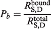where the numerator is the number of observed occurrences of residue R bound to a ligand in the training set. It is normalized by the total number of such residues found in the same depth-SASA category.

Identifying binding cavities

When predicting binding cavities on a protein, its residue-wise SASA and depth are first computed. Probability values are assigned corresponding to its residue depth and SASA categories. All residues with probability values above a threshold are selected as binding cavity residues. The protein is then resolvated (25 cycles by default). This time only clashing waters are removed. Water molecules that are within 4.2 Å from any of the selected residues are inspected. An inspected water molecule is retained if there is at least one other water molecule within 4.2 Å of it. The rest of the waters are not considered. All protein residues that are within a distance of 4.2 Å from the retained water molecules are also considered as residues lining the binding cavity. A continuous patch of these residues constitutes an independent binding cavity linings prediction.

Training and testing sets

Three hundred and twenty-five structures of single and multi-chain proteins listed in LigASite v7.0 (31) holo structure (bound to small molecule ligands) data set were obtained from the Protein Quaternary Structure (PQS) server (32). These structures were randomly bifurcated into a training set of 100 and a testing set of 225 with average chain lengths of 282 and 245, respectively. The training and testing sets consisted of 62 and 133 multi-chain PDB files, respectively. Details of the training and testing sets can be found in Supplementary Data (http://mspc.bii.a-star.edu.sg/tankp/stat_files/train-set_and_ligand).

Parameter optimization

Predictions of residues that line the binding cavity were made using DEPTH by varying the minimum number of neighborhood waters (n) in the range (2–5) in steps of one and the binding probability threshold (P) in the range 0.10–0.80 in steps of 0.05 over the training set. Residues were classified as belonging to binding site or non-binding site. The set of parameters (n = 4 and P = 0.50) that gave us the best Matthews correlation coefficient (MCC) (33) were chosen as the optimal values for our method and are the default values on the server. The MCC was computed as

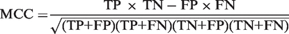where TP, TN, FP and FN represent the numbers of true positive, true negative, false positive and false negative, respectively.

RESULTS

Residue depth preference of the different amino acids

The depth profiles of the 20 amino acid types correlate strongly with their biochemical properties. The depth values of all residues in a set of 1457 structures (see Supplementary Data—http://mspc.bii.a-star.edu.sg/depth/stats.html for details) were computed. All amino acid residues show a peak in the distribution at low depth values (3–4 Å). Hydrophobic amino acids (ALA, ILE, LEU, MET, PHE, VAL, TRP and TYR) and CYS showed a higher tolerance for deep environments than other residues, with a second peak in the distribution at around 7 Å. In contrast, charged and large polar groups of amino acids (ARG, ASN, ASP, GLU, GLN, HIS and LYS) have a lower propensity to be in deep environments. The same trend was noticed for PRO. Smaller polar amino acids SER and THR along with GLY exhibit a similar trend albeit with a relatively larger tail of the distribution at deep environments.

Applications of residue depth

Residue depth values are useful in computing and estimating several important physical properties related to the structure of proteins. The deepest residues usually, unambiguously, identify the protein core. Residue depth has been earlier shown to correlate well with hydrogen exchange rates (1,3) and thermal stability under mutagenesis (1). Depth can hence be a useful measure in the prediction of protein–protein interaction hot spots (1), detecting sites for post-translational modification (5,6) and predicting the effect of point mutations on protein stability and function (1,4,5). Given that the depth computation is simple and rapid, it may also be an attractive tool to analyze molecular dynamics trajectories and to evaluate the accuracy of protein structure models. In the next section, we illustrate the utility of the depth measure with an application to predict small molecule ligand binding sites on proteins.

Prediction of small molecule ligand binding sites

We showcase one application of the depth measure by predicting the protein residues that would interact with ligands. We have compared the results from DEPTH to LIGSITE (12), Pocket-Finder (7), SURFNET (15) and ConCavity (9). ConCavity incorporates both structural and evolutionary information while the other methods rely only on structural geometry of the proteins. In our tests, ConCavity was run using LIGSITE for structural geometry and evolutionary information for the queries were taken from the ConCavity web site (http://compbio.cs.princeton.edu/concavity/pqs/jsd/). The probability value threshold for ConCavity for binary classification was set at 0.085. LIGSITE, Pocket-Finder and SURFNET were also run from within the ConCavity program, with all parameters set to their default values, and without the use of evolutionary information. For DEPTH, the minimum number of neighborhood waters and threshold probability values were set to 4 and 0.50, respectively, which are our recommended values for multi-chain protein binding site prediction.

MCC was computed for DEPTH and the other methods over the testing set data. While ConCavity outperforms all other methods, the overall performance of DEPTH is comparable to that of the structure based methods (Table 1). DEPTH outperforms the structure-based methods when tested over multi-chain proteins. However, DEPTH is marginally poorer (MCC = 0.44) than the other structure-based programs (MCC values in the range 0.46–0.53) when tested over single-chain proteins.

Table 1.

The Matthew’s correlation values for the DEPTH^a (bold face), LIGSITE^b, Pocket-Finder^c, SURFNET^d and ConCavity^e over the testing data set of 225 single (92) and multi-chain (133) proteins

Single-chain PDBs (92)					Multi-chain PDBs (133)					Entire testing set (225)
Da	Lb	Pc	Sd	Ce	D	L	P	S	C	D	L	P	S	C
0.44	0.53	0.48	0.47	0.50	0.39	0.37	0.37	0.38	0.48	0.39	0.40	0.39	0.39	0.49

DEPTH overpredicts the number of binding residues. On average, the size of binding site in the testing set is 65 residues per structure. On an average, DEPTH predicts 105 while ConCavity, LIGSITE, POCKET and SURFNET predict 98, 94, 93 and 103 residues, respectively. These overpredictions contribute significantly to the number of false positives.

Software and web server adjustable parameters

Our program computes depth at the atomic/residue level and as an application, predicts the location of small molecule binding sites. The web server (Figure 1) is freely accessible without login requirements at http://mspc.bii.a-star.edu.sg/depth. Users specify the four-letter PDB code of a protein or upload a file in PDB format. Users are also given the option to tune several parameters. For residue depth computation, the minimum number of neighborhood waters, solvent neighborhood radius and the number of solvation cycles can all be tuned to cater for different accuracies. For binding cavity predictions, the default values of minimum number of neighboring waters and threshold probability were set to 4 and 0.50, respectively. Users can override these values, for instance, when predicting binding sites in single- or multi-domain proteins. Help pages provide information on the program, server and the different parameters with their optimal values and limits.

Figure 1.

Snapshots of the input and output pages of the server (http://mspc.bii.a-star.edu.sg/tankp/). (A) The input page showing all the tunable parameters. (B) The output associated with residue depth computation, including a 2D plot of residue-wise depth and a surface representation of the query protein (PDB 2FP7) rainbow-colored according to depth. The deeper is a residue the bluer it is colored. (C) Modified snapshot of the output of the binding cavity prediction for PDB 2FP7. The 2D plot shows the residue-wise probability values and the probability threshold. The predicted binding site residues are listed below the plot. The accompanying surface representation of the protein has the predicted binding cavity residues colored in red while the rest of the protein is colored blue. The inhibitor is shown in white stick representation to highlight the flat geometry of the binding site.

Server output

For residue depth computation, a summary of residue depth computation parameters is displayed on the output page. By default, the query protein 3D structure is displayed in a Jmol viewer and rainbow-colored by residue-wise depth. The bluer a residue the more buried it is in the structure. Plots of residue depths of selected groups of atoms of a residue (main chain, side chain, polar and non-polar) can also be displayed according to user specification. Users have the option to download the output of atomic/residue depth and SASA values in tab delimited and/or PDB format. All results will be stored for 30 days before they are cleared. For binding cavity prediction, a residue binding cavity probability plot with user-defined and recommended threshold is displayed. The 3D structure of the query protein is displayed in a Jmol viewer with predicted binding cavity residues colored in red. The Jmol menu can be used to render the output as desired. Residue-wise probability values are downloadable in tab delimited or PDB format. A stand-alone version of the depth and SASA programs is available for download if users wish to use it locally.

Case study: West Nile Virus NS2B/NS3 protease

We illustrate the use of our server by running the depth calculation and ligand binding site prediction on West Nile Virus NS2B/NS3 protease (PDB:2FP7). The protease is a protein complex of two chains (chain A:NS2B and chain B:NS3), 47 and 148 amino acid residues long, respectively. The substrate binding site of the protease is located at the interface between the two chains and consists of amino acid residues from both chains (D82:A, G83:A, N84:A, F85:A, Q86:A and H51:B, D75:B, D129:B, Y130:B, P131:B, T132:B, Y150:B, G151:B, N152:B, G153:B, Y161:B) (34).

Residue depth computation

Four sets of depth results were obtained by varying the minimum number of neighborhood waters from two to five. The solvent neighborhood radius was retained at its default value 4.2 Å. Increasing the number of minimum neighborhood waters increases the mean and maximum of residue depths monotonically, from 5.25 and 11.79 to 6.76 Å and 14.17 Å, respectively. This happens because an increase in the minimum number of neighborhood waters excludes a larger number of cavity solvent molecules, resulting in greater depth values. The depth values increased the most at two regions on the protein, centered around V166:B (6.87–12.74 Å) and N152:B (5.22–8.98 Å). Such transitions are usually indicative of shallow cavities that are difficult to detect using methods that rely on structural geometry alone.

Binding site residue prediction

The probability threshold value controls the stringency of the prediction. Usually, the higher is the probability threshold value the fewer are the binding cavities detected. Increasing the number of minimum neighborhood waters (this number is recommended not to exceed five) usually results in a prediction of a larger number of binding site residues. In addition, it also facilitates the detection of geometrically flatter binding cavities.

In the case of the West Nile Virus protease, no binding sites were predicted at the default values of number of neighborhood waters (n = 4) and probability threshold (P = 0.50). Increasing the minimum number of neighborhood waters to 5 and decreasing the probability threshold to 0.45 resulted in the detection of a relatively flat binding site centered around residue N152:B (Figure 1C). Our prediction correctly identifies 9 of the 16 binding site residues. Except for ConCavity, none of the other methods tested here were able to correctly identify this binding site.

CONCLUSIONS

In this study, we present a program to compute atomic/residue depths quickly and accurately. The web server associated with the program also computes SASA values. Residue depth provides a gradually stratified profile of residue/atomic burial with an appreciably larger dynamic range of burial as compared to SASA. Generally, residue depth values show a trend that is the inverse of SASA values. The solvent exposed residues usually have low depth values while the less exposed residues are deeper in the protein.

Exceptions to this trend appear in most protein structures when solvent exposed residues have large depth values. Our investigation, over a set of 900 proteins, revealed that such residues are often part of small molecule ligand binding cavities. From this set of 900 proteins, we have estimated the likelihood of the 20 different amino acids to be part of the binding cavity given their depth and SASA values. These likelihood values are then used to predict residues that line binding site cavities. After we identify one or more residues in a cavity, we include its closest solvent exposed neighbors to increase coverage.

We tested the performance of our predictions against other popular methods including ConCavity, LIGSITE, Pocket-Finder and SURFNET over a set of 225 single and multi-chain structures of proteins known to bind small molecule ligands. With optimal parameters, DEPTH performs on par with all the other methods except ConCavity. ConCavity uses evolutionary information in addition to protein structure geometry and outperforms all other methods. It is likely that DEPTH too could benefit from evolutionary information.

We have demonstrated the effects of changing the parameters of the algorithm and how binding cavities of different sizes and properties can be detected. One of the benefits of cavity detection with DEPTH is its ability to pick out shallow binding pockets, as exemplified in the case of the West Nile Virus Protease.

Residue depth has been shown earlier to have many potential applications. This server has been setup primarily to provide accurate depth values that users could use for several applications, some of which have been listed on the server. In addition, we showcased the usefulness of depth values with one application—predicting small molecule binding sites. The prediction method is coarse grained and yet performs comparably to other more established and sophisticated structure based methods. This encourages us to explore other applications, which we hope to add to the server in the future.

SUPPLEMENTARY DATA

Supplementary Data are available at NAR Online.

FUNDING

Funding for open access charge: Biomedical Research Council (A*STAR), Singapore.

Conflict of interest statement. None declared.

REFERENCES

- 1.Chakravarty S, Varadarajan R. Residue depth: a novel parameter for the analysis of protein structure and stability. Structure. 1999;7:723–732. doi: 10.1016/s0969-2126(99)80097-5. [DOI] [PubMed] [Google Scholar]
- 2.Lee B, Richards FM. The interpretation of protein structures: estimation of static accessibility. J. Mol. Biol. 1971;55:379–400. doi: 10.1016/0022-2836(71)90324-x. [DOI] [PubMed] [Google Scholar]
- 3.Pedersen TG, Sigurskjold BW, Andersen KV, Kjaer M, Poulsen FM, Dobson CM, Redfield C. A nuclear magnetic resonance study of the hydrogen-exchange behaviour of lysozyme in crystals and solution. J. Mol. Biol. 1991;218:413–426. doi: 10.1016/0022-2836(91)90722-i. [DOI] [PubMed] [Google Scholar]
- 4.Pintar A, Carugo O, Pongor S. Atom depth as a descriptor of the protein interior. Biophys. J. 2003;84:2553–2561. doi: 10.1016/S0006-3495(03)75060-7. [DOI] [PMC free article] [PubMed] [Google Scholar]
- 5.Pintar A, Carugo O, Pongor S. Atom depth in protein structure and function. Trends Biochem. Sci. 2003;28:593–597. doi: 10.1016/j.tibs.2003.09.004. [DOI] [PubMed] [Google Scholar]
- 6.Pintar A, Pongor S. The ‘first in-last out’ hypothesis on protein folding revisited. Proteins. 2005;60:584–590. doi: 10.1002/prot.20529. [DOI] [PubMed] [Google Scholar]
- 7.An J, Totrov M, Abagyan R. Pocketome via comprehensive identification and classification of ligand binding envelopes. Mol. Cell. Proteomics. 2005;4:752–761. doi: 10.1074/mcp.M400159-MCP200. [DOI] [PubMed] [Google Scholar]
- 8.Brady GP, Jr, Stouten PF. Fast prediction and visualization of protein binding pockets with PASS. J. Comput. Aided Mol. Des. 2000;14:383–401. doi: 10.1023/a:1008124202956. [DOI] [PubMed] [Google Scholar]
- 9.Capra JA, Laskowski RA, Thornton JM, Singh M, Funkhouser TA. Predicting protein ligand binding sites by combining evolutionary sequence conservation and 3D structure. PLoS Comput. Biol. 2009;5:e1000585. doi: 10.1371/journal.pcbi.1000585. [DOI] [PMC free article] [PubMed] [Google Scholar]
- 10.Del Carpio CA, Takahashi Y, Sasaki S. A new approach to the automatic identification of candidates for ligand receptor sites in proteins: (I). Search for pocket regions. J. Mol. Graph. 1993;11:23–29, 42. doi: 10.1016/0263-7855(93)85003-9. [DOI] [PubMed] [Google Scholar]
- 11.Delaney JS. Finding and filling protein cavities using cellular logic operations. J. Mol. Graph. 1992;10:174–177, 163. doi: 10.1016/0263-7855(92)80052-f. [DOI] [PubMed] [Google Scholar]
- 12.Hendlich M, Rippmann F, Barnickel G. LIGSITE: automatic and efficient detection of potential small molecule-binding sites in proteins. J. Mol. Graph. Model. 1997;15:359–363, 389. doi: 10.1016/s1093-3263(98)00002-3. [DOI] [PubMed] [Google Scholar]
- 13.Ho CM, Marshall GR. Cavity search: an algorithm for the isolation and display of cavity-like binding regions. J. Comput. Aided Mol. Des. 1990;4:337–354. doi: 10.1007/BF00117400. [DOI] [PubMed] [Google Scholar]
- 14.Kleywegt GJ, Jones TA. Detection, delineation, measurement and display of cavities in macromolecular structures. Acta Crystallogr. D Biol. Crystallogr. 1994;50:178–185. doi: 10.1107/S0907444993011333. [DOI] [PubMed] [Google Scholar]
- 15.Laskowski RA. SURFNET: a program for visualizing molecular surfaces, cavities, and intermolecular interactions. J. Mol. Graph. 1995;13:323–330, 307–328. doi: 10.1016/0263-7855(95)00073-9. [DOI] [PubMed] [Google Scholar]
- 16.Laurie AT, Jackson RM. Q-SiteFinder: an energy-based method for the prediction of protein-ligand binding sites. Bioinformatics. 2005;21:1908–1916. doi: 10.1093/bioinformatics/bti315. [DOI] [PubMed] [Google Scholar]
- 17.Le Guilloux V, Schmidtke P, Tuffery P. Fpocket: an open source platform for ligand pocket detection. BMC Bioinformatics. 2009;10:168. doi: 10.1186/1471-2105-10-168. [DOI] [PMC free article] [PubMed] [Google Scholar]
- 18.Levitt DG, Banaszak LJ. POCKET: a computer graphics method for identifying and displaying protein cavities and their surrounding amino acids. J. Mol. Graph. 1992;10:229–234. doi: 10.1016/0263-7855(92)80074-n. [DOI] [PubMed] [Google Scholar]
- 19.Liang J, Edelsbrunner H, Woodward C. Anatomy of protein pockets and cavities: measurement of binding site geometry and implications for ligand design. Protein Sci. 1998;7:1884–1897. doi: 10.1002/pro.5560070905. [DOI] [PMC free article] [PubMed] [Google Scholar]
- 20.Masuya M, Doi J. Detection and geometric modeling of molecular surfaces and cavities using digital mathematical morphological operations. J. Mol. Graph. 1995;13:331–336. doi: 10.1016/0263-7855(95)00071-2. [DOI] [PubMed] [Google Scholar]
- 21.Peters KP, Fauck J, Frommel C. The automatic search for ligand binding sites in proteins of known three-dimensional structure using only geometric criteria. J. Mol. Biol. 1996;256:201–213. doi: 10.1006/jmbi.1996.0077. [DOI] [PubMed] [Google Scholar]
- 22.Venkatachalam CM, Jiang X, Oldfield T, Waldman M. LigandFit: a novel method for the shape-directed rapid docking of ligands to protein active sites. J. Mol. Graph. Model. 2003;21:289–307. doi: 10.1016/s1093-3263(02)00164-x. [DOI] [PubMed] [Google Scholar]
- 23.Weisel M, Proschak E, Schneider G. PocketPicker: analysis of ligand binding-sites with shape descriptors. Chem. Cent. J. 2007;1:7. doi: 10.1186/1752-153X-1-7. [DOI] [PMC free article] [PubMed] [Google Scholar]
- 24.Leis S, Schneider S, Zacharias M. In silico prediction of binding sites on proteins. Curr. Med. Chem. 2010;17:1550–1562. doi: 10.2174/092986710790979944. [DOI] [PubMed] [Google Scholar]
- 25.Schmidtke P, Souaille C, Estienne F, Baurin N, Kroemer RT. Large-scale comparison of four binding site detection algorithms. J. Chem. Inf. Model. 2010;50:2191–2200. doi: 10.1021/ci1000289. [DOI] [PubMed] [Google Scholar]
- 26.Berendsen HJC, Grigera JR, Straatsma TP. The missing term in effective pair potentials. J. Phys. Chem. 1987;91:6269–6271. [Google Scholar]
- 27.Berendsen HJC, Postma JPM, Gunsteren WFv, Hermans J. In Intermolecular Forces. D. Reidel Publishing Company, Dordrecht; 1981. [Google Scholar]
- 28.Shrake A, Rupley JA. Environment and exposure to solvent of protein atoms. Lysozyme and insulin. J. Mol. Biol. 1973;79:351–371. doi: 10.1016/0022-2836(73)90011-9. [DOI] [PubMed] [Google Scholar]
- 29.Hubbard TJ, Blundell TL. Comparison of solvent-inaccessible cores of homologous proteins: definitions useful for protein modelling. Protein Eng. 1987;1:159–171. doi: 10.1093/protein/1.3.159. [DOI] [PubMed] [Google Scholar]
- 30.Berman HM, Westbrook J, Feng Z, Gilliland G, Bhat TN, Weissig H, Shindyalov IN, Bourne PE. The Protein Data Bank. Nucleic Acids Res. 2000;28:235–242. doi: 10.1093/nar/28.1.235. [DOI] [PMC free article] [PubMed] [Google Scholar]
- 31.Dessailly BH, Lensink MF, Orengo CA, Wodak SJ. LigASite–a database of biologically relevant binding sites in proteins with known apo-structures. Nucleic Acids Res. 2008;36:D667–D673. doi: 10.1093/nar/gkm839. [DOI] [PMC free article] [PubMed] [Google Scholar]
- 32.Henrick K, Thornton JM. PQS: a protein quaternary structure file server. Trends Biochem. Sci. 1998;23:358–361. doi: 10.1016/s0968-0004(98)01253-5. [DOI] [PubMed] [Google Scholar]
- 33.Matthews BW. Comparison of the predicted and observed secondary structure of T4 phage lysozyme. Biochim. Biophys. Acta. 1975;405:442–451. doi: 10.1016/0005-2795(75)90109-9. [DOI] [PubMed] [Google Scholar]
- 34.Erbel P, Schiering N, D’Arcy A, Renatus M, Kroemer M, Lim SP, Yin Z, Keller H, Vasudevan SG, Hommel U. Structural basis for the activation of flaviviral NS3 proteases from dengue and West Nile virus. Nat. Struct. Mol. Biol. 2006;13:372–373. doi: 10.1038/nsmb1073. [DOI] [PubMed] [Google Scholar]