Design of the lac gene circuit revisited

Abstract

The lactose (lac) operon of Escherichia coli serves as the paradigm for gene regulation, not only for bacteria, but also for all biological systems from simple phage to humans. The details of the systems may differ, but the key conceptual framework remains, and the original system continues to reveal deeper insights with continued experimental and theoretical study. Nearly as long lasting in impact as the pivotal work of Jacob and Monod is the classic experiment of Novick and Weiner in which they demonstrated all-or-none gene expression in response to an artificial inducer. These results are often cited in claims that normal gene expression is in fact a discontinuous bistable phenomenon. In this paper, I review several levels of analysis of the lac system and introduce another perspective based on the construction of the system design space. These represent variations on a theme, based on a simply stated design principle, that captures the key qualitative features of the system in a largely mechanism-independent fashion. Moreover, this principle can be readily interpreted in terms of specific mechanisms to make predictions regarding monostable vs. bistable behavior. The regions of design space representing bifurcations are compared with the corresponding regions identified through bifurcation analysis. I present evidence based on biological considerations as well as modeling and analysis to suggest that induction of the lac system in its natural setting is a monostable continuously graded phenomenon. Nevertheless, it must be acknowledged that the lac stability question remains unsettled, and it undoubtedly will remain so until there are definitive experimental results.

1. Introduction

Ever since the groundbreaking work of Jacob and Monod [1], the lactose (lac) system has continued to serve as the paradigm of gene regulation [2–4]. The concepts that were first introduced are still in place today, even as some of the terms currently used to describe them have changed: structural gene, transcription factor, transcription-factor binding sites, promoter region. Repressor control and constitutive synthesis of repressor also were influential features of the original model, but have long since been generalized to include activator control and coupled expression of regulator and effector functions. Indeed, there are now well-documented rules that account for both the mode of molecular control [5,6,7] and the coupling of regulator and effector expression [8–10].

One of the other lasting impacts of the lac system is the classic paper by Novick and Weiner [11] in which they demonstrated an all-or-none response to the artificial non-metabolizable inducer thio-methylgalactoside (TMG). Humans by nature are more drawn to phenomena that manifest excitability, oscillations and sharp thresholds rather than those that exhibit more prosaic regular behavior. Hence, it is not surprising that one of the first hints of a molecular mechanism exhibiting memory might have this impact and that gene expression might often be considered (uncritically) all-or-none.

Indeed, the early mathematical models focused on the obvious positive feedback and cooperativity in this artificial system and were able to mimic the all-or-none hysteretic behavior (e.g., [12–14]). However, at this time there were still key features of the lac system that had not been discovered, never mind that there was no experimental evidence for such a response in the natural system with lactose as substrate. One of these features was the discovery that allolactose is the natural inducer in this system; it is an intermediate in the catabolism of lactose being both produced and removed by the enzyme β-galactosidase [15]. Even with this key feature included in the models there was a concerted effort to show that the natural system was hysteretic, and when models were found to exhibit hysteresis, the unjustified claim was often made that the results were supported by the experimental data of Novick and Weiner. In much of this work there was little if any consideration given to the physiological role of this system in the organism.

In my own early modeling of the lac system, I found that when the inducer was an intermediate or substrate of the inducible system, it had a profound impact on stability and made it more difficult to produce the instability necessary for the hysteretic induction [16]. Moreover, this and subsequent analyses were done in the context of several performance criteria for the physiological function of this system including robustness, cost/benefit considerations, and response times [8,9, 16–18]. These results pointed in the direction of monostable rather than bistable induction.

The condition for bistability in all these studies can be expressed compactly (in a mechanism-independent fashion) in terms of a difference in aggregate kinetic orders with respect to β-galactosidase for production g₃₂ and removal g₅₂ of inducer, and the inverse of the effective cooperativity with which inducer influences mRNA synthesis g₁₄ :

$$(g_{32}-g_{52})>\frac{h_{11}{h}_{22}{g}_{54}}{g_{21}}\frac{1}{g_{14}}$$

The meaning of this condition, including the definition of all its parameters and its interpretation in various contexts, will become clear in the following sections. Although this condition is mechanism independent, the aggregate kinetic orders can be readily interpreted in terms of specific mechanisms, such as inducer exclusion [19], catabolite repression via the global regulator CRP [20], the export of intermediates [21–24], growth-rate dependent dilution [25,26], auxiliary operator sites, and the details of repressor binding [27,28]. For these cases, a more general and compact expression of the condition for bistability is (−1)ⁿ Δ_n < 0, where Δ_n is the determinant of the system matrix involving the aggregate kinetic orders for the dependent variables [16].

There are more recent modeling efforts that support our predictions of monostability for the natural system with lactose as substrate [29] as well as continuing efforts to demonstrate bistability in such models [30]. The stability question appears to remain unsettled, and it will probably remain so until the definitive experimental results are in.

Recently, my colleagues and I have introduced the concept of a “system design space” that provides another way for us to view the design of the lac system. In this space, the qualitatively distinct phenotypes of a biochemical system can be identified, counted, analyzed, and compared [31]. Boundaries in design space indicate a transition between phenotypic behaviors and can be used to measure a system’s tolerance to large changes in parameters [32]. The system design space approach has been used to study control of lysogeny in bacterophage lambda [33], population dynamics of gene duplications in Salmonella enterica [34], and regulation of a global transcription factor in E. coli [35]. We have also automated the construction and analysis of design space by implementing the algorithms in the Design Space Toolbox for MATLAB [36].

In this paper I will review the several types of analyses that we have used previously, highlight their advantages and disadvantages, and turn to the analysis in the context of system design space. In the process I shall be returning to the familiar example of the lac system and the design principle mentioned above with a view to examining two questions regarding graded induction vs. all-or-none switching. First, there are aspects of the larger circuitry in which the lac system participates that models have suggested might influence the switching behavior of the lac system [17, 25, 26, 30, 37]. These include inducer exclusion, catabolite repression via the global regulator CRP, glucose transport, alternative fates for the intermediates, and growth-rate dependent dilution. Second, a reexamination of graded induction vs. all-or-none switching from the perspective of system design space will provide an opportunity to compare its boundaries with those defined by traditional bifurcation analysis [38,39].

It should be emphasized that our focus is on the essential features of the system and their qualitative implications. The goal is to elucidate robust aspects of the design for an entire class of systems and that are thus independent of other mechanistic differences that are always found in particular systems. Moreover, the numerical values of the numerous parameters that would be necessary to fully characterize even a single system in situ are simply not available. Thus, our approach can be contrasted with others that attempt to estimate parameter values and focus on quantitative details of kinetic mechanism, time delay and stochastic effects (for excellent reviews see [26, 40]). When successful, these are likely to add quantitative detail, but are unlikely to change our qualitative results. In addition to the older experimental literature, there are now single cell measurements that have addressed the question of bistability [41,42] and these will be discussed in relation to our theoretical predictions.

2. Core lac circuitry

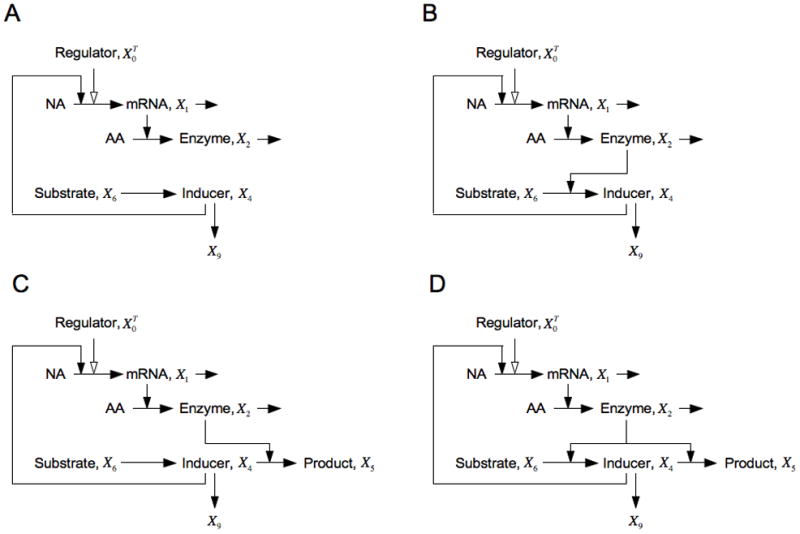
Figure 1 is a graphical representation of the interactions that make up the core lac circuitry. The salient features include quadratic kinetics of induction as a function of inducer, first-order loss of mRNA and protein, coordinate expression of pathway enzymes encoded in a polycystronic message, low turnover of β-galactosidase enzyme, and high turnover of intermediate inducer. Figure 2 is a graphical depiction of a steady-state induction characteristic [16] in which the steady-state level of gene expression is plotted on the y-axis as a function of the steady-state level of inducer on the x-axis in logarithmic coordinates.

Fig. 1.

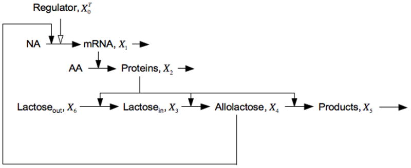
Model of the core interactions in the lactose system. The pools of nucleotides and amino acids are assumed to be constant and are not shown with explicit variables. The polycistronic messenger RNA encodes proteins that include a permease for the transport of extracellular lactose into the cell, the enzyme β-galactosidase that catalyzes both the synthesis and degradation of the inducer allolactose, as well as a transacetylase that is not represented. The regulator is a repressor of transcription and its level is constitutively expressed. Filled arrows represent interactions that are positive, open arrows those that are negative.

Fig. 2.

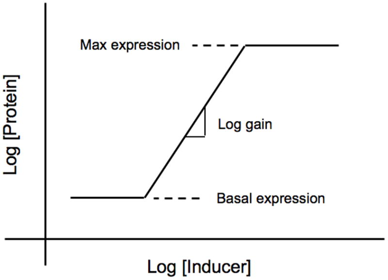
Idealized steady-state induction characteristic. Cells are grown for several generations in fixed concentrations of inducer to achieve a steady state and the resulting level of gene expression is determined. Gene expression can be measured in several ways, but the most common is to measure the level of an encoded protein, as is show in this illustration. The results are plotted in log-log coordinates. At sub-threshold concentrations of inducer there is a basal level of expression. At high concentrations of inducer there is a maximal level of expression. At intermediate levels of inducer there is a region of regulated expression in which the slope is quantified by the logarithmic gain in expression.

Most of our previous analyses of inducible catabolic systems such as the lac system have used the local S-system representation within the power-law formalism. This is rigorously justified as long as the system operates within a defined neighborhood of a steady state. Under these conditions the local representation has a number of advantages regarding the symbolic analysis of the system [16,43]. The analysis in this section will provide a useful reference for comparisons in later sections when we consider other mechanisms, systems that may or may not be stable, and responses that may not remain within the defined neighborhood of a steady state.

Let us briefly reiterate the local analysis of this system [16], with a specific focus on the stability of the solution in the regulatable region of the induction characteristic. The S-system equations are the following:

$$\begin{array}{l}\frac{{dX}_1}{dt}={\alpha }_1{X}_0^{g_{10}}{X}_4^{g_{14}}-{\beta }_1{X}_1^{h_{11}}\\ \frac{{dX}_2}{dt}={\alpha }_2{X}_1^{g_{21}}-{\beta }_2{X}_2^{h_{22}}\\ \frac{{dX}_3}{dt}={\alpha }_3{X}_2^{g_{32}}{X}_6^{g_{36}}-{\alpha }_4{X}_2^{g_{42}}{X}_3^{g_{43}}\\ \frac{{dX}_4}{dt}={\alpha }_4{X}_2^{g_{42}}{X}_3^{g_{43}}-{\alpha }_5{X}_2^{g_{52}}{X}_4^{g_{54}}\\ \frac{{dX}_5}{dt}={\alpha }_5{X}_2^{g_{52}}{X}_4^{g_{54}}-{\alpha }_7{X}_5^{g_{75}}\end{array}$$ (1)

(Although the standard notation for the loss of X₅ would typically use parameters β₅ and h₅₅, the choice in this case will make more sense when comparisons are made in Section 4.) This representation, guaranteed by Taylor’s theory to be locally valid about any steady state, is important because it captures the essential local behavior in a mechanism independent but architecturally dependent fashion, as will become evident from the conclusions in this and in later sections.

2.1. Steady State

Setting the derivatives in Eqns. (1) to zero, rearranging terms, and taking logarithms yields the following linear system:

$$\begin{array}{l}-h_{11}{y}_1+g_{14}{y}_4=log({\beta }_1/{\alpha }_1)-g_{10}{y}_{10}\\ g_{21}{y}_1-h_{22}{y}_2=log({\beta }_2/{\alpha }_2)\\ (g_{32}-g_{42})y_2-g_{43}{y}_3=log({\alpha }_4/{\alpha }_3)-g_{36}{y}_6\\ (g_{42}-g_{52})y_2+g_{43}{y}_3-g_{54}{y}_4=log({\alpha }_5/{\alpha }_4)\\ g_{52}{y}_2+g_{54}{y}_4-g_{75}{y}_5=log({\alpha }_7/{\alpha }_5)\end{array}$$ (2)

where y_i = log X_i. This system of linear equations can be readily solved for the logarithm of the protein concentration y₂.

$$y_2=\frac{g_{54}\{g_{21}[g_{10}{y}_0-log({\beta }_1/{\alpha }_1)]-h_{11}log({\beta }_2/{\alpha }_2)\}+g_{12}{g}_{14}[g_{36}{y}_6-log({\alpha }_5/{\alpha }_3)]}{h_{11}{h}_{22}{g}_{54}-g_{21}{g}_{14}(g_{32}-g_{52})}$$ (3)

where Δ₅ = g₇₅[g₂₁g₁₄ (g₃₂ − g₅₂ ) − h₁₁h₂₂g₅₄] ≠ 0 is the determinant of the system matrix in Eqns. (2).

The slope for the regulatable region of the steady-state induction characteristic, when expression is measured in terms of protein levels, is then given by the logarithmic gain L(X₂, X₆) = ∂y₂/∂y₆ [16].

$$L(X_2,X_6)=\frac{g_{21}{g}_{14}{g}_{36}}{h_{11}{h}_{22}{g}_{54}-g_{21}{g}_{14}(g_{32}-g_{52})}$$ (4)

Note that all the parameters in this equation are positive and that there is a condition on the denominator (or the determinant of the kinetic orders for the dependent variables) for this logarithmic gain to be positive (and finite!) as it must be for a graded inducible system; namely,

$$(g_{32}-g_{52})<\frac{h_{11}{h}_{22}{g}_{54}}{g_{21}{g}_{14}}$$ (5)

or (−1)⁵Δ₅ > 0. This is one manifestation of the design principle mentioned in the introduction. We will see this critical condition appear later in other contexts.

The steady-state solution also can be described from a graphical point of view [17, 43]. The “open-loop transfer function” from X₄ to X₂ in steady state is obtained by solving the first two of Eqns. (2) when X₀ is fixed and X₄ is considered an independent variable. The result,

$$y_2=[g_{10}{g}_{21}{y}_0+g_{21}{g}_{14}{y}_4-g_{21}log({\beta }_1/{\alpha }_1)-h_{11}log({\beta }_2/{\alpha }_2)]/(h_{11}{h}_{22})$$ (6)

is the equation of a straight line with slope s₁ = g₂₁g₁₄/(h₁₁h₂₂ ) in logarithmic space. It is also the logarithmic gain L(X₂, X₄ ) = ∂y₂/∂y₄ = g₂₁g₁₄/(h₁₁h₂₂ ) in the regulatable region. This value of X₂ is proportional to the steady-state rate of synthesis of X₂ as a function of X₄ when noting the first-order processes in the first two of Eqns. (1); in steady state the rate of X₂ synthesis is given by α₂ X₁ and X₂ is proportional to X₁.

Similarly, the “open-loop transfer function” from X₂ to X₄ in steady state is obtained by solving the third and fourth of Eqns. (2) when X₂ is considered an independent variable. The result is

$$y_4=[(g_{32}-g_{52})y_2+g_{36}{y}_6-log({\alpha }_5/{\alpha }_3)]/g_{54}$$

with logarithmic gain L(X₄, X₂ ) in the regulatable region. Inverting this equation yields

$$y_2=[log({\alpha }_5/{\alpha }_3)-g_{36}{y}_6+g_{54}{y}_4]/(g_{32}-g_{52})$$ (7)

In this case, the slope of the resulting line in logarithmic space is s₂ = g₅₄/(g₃₂ − g₅₂ ). This value of X₂ also is proportional to the steady-state rate of degradation of X₂ as a function of X₄.

A unique steady-state solution is determined by the intersection of the two transfer functions. Here it is sufficient to note the relative slopes of these transfer functions. The results are shown for s₁ > s₂ > 0 in Fig. 3A, s₂ > s₁ > 0 in Fig. 3B, and s₁ > 0 > s₂ in Fig. 3C. These three cases correspond to one eigenvalue that is positive real, no eigenvalues with positive real parts, and two eigenvalues with positive real parts, as will become clear when these are explored later in more detail. Note that the last of Eqns. (2) is irrelevant for this analysis, since X₅ simply follows from X₄. We have included it here in order to facilitate comparisons that will be made in Section 4.

Fig. 3.

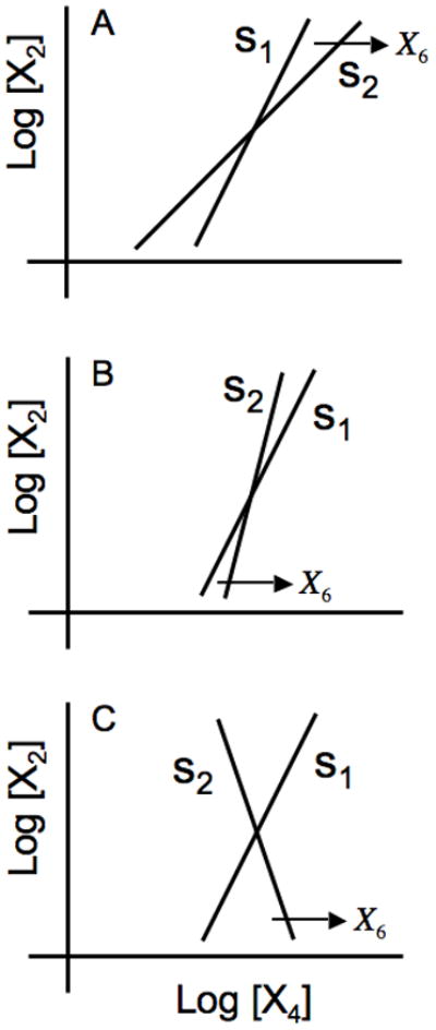
Graphical depiction of the steady-state solutions in the local power-law representation. The open-loop transfer function from X₄ to X₂ is represented by the line with slope s₁ ; that from X₂ to X₄ is represented by the line with slope s₂ whose horizontal displacement is a function of the substrate concentration X₆. (A) s₁ > s₂ > 0. (B) s₂ > s₁ > 0, and (C) s₁ > 0 > s₂. See text for discussion.

2.2. Stability

The local dynamic equations about any nominal steady state in the regulatable region are the following [16]:

$$\begin{array}{l}\frac{{du}_1}{dt}=F_1[-h_{11}{u}_1+g_{14}{u}_4]\\ \frac{{du}_2}{dt}=F_2[g_{21}{u}_1-h_{22}{u}_2]\\ \frac{{du}_3}{dt}=F_3[(g_{32}-g_{42})u_2-g_{43}{u}_3]\\ \frac{{du}_4}{dt}=F_4[(g_{42}-g_{52})u_2+g_{43}{u}_3-g_{54}{u}_4]\\ \frac{{du}_5}{dt}=F_5[g_{52}{u}_2+g_{54}{u}_4-g_{75}{u}_5]\end{array}$$ (8)

where u_i = y_i − y_i0, F_i = V_i0/X_i0 and the additional subscript ₀ signifies the values at a particular steady state. From these we obtain the characteristic equation (whose solutions λ are the eigenvalues of the response), which can be written as

$$(\lambda +F_5{g}_{75})[{\lambda }^4+{\theta }_1{\lambda }^3+{\theta }_2{\lambda }^2+{\theta }_3\lambda +{\theta }_4]=0$$ (9)

$$\begin{array}{l}\text{with}{\theta }_1=F_1{h}_{11}+F_2{h}_{22}+F_3{g}_{43}+F_4{g}_{54}>0,\\ {\theta }_2=F_1{F}_2{h}_{11}{h}_{22}+F_1{F}_3{h}_{11}{g}_{43}+F_1{F}_4{h}_{11}{g}_{54}+F_2{F}_3{h}_{22}{g}_{43}+F_2{F}_4{h}_{22}{g}_{54}+F_3{F}_4{g}_{43}{g}_{54}>0,\\ {\theta }_3=F_1{F}_2{F}_3{h}_{11}{h}_{22}{g}_{43}+F_1{F}_2{F}_4[h_{11}{h}_{22}{g}_{54}-g_{21}{g}_{14}(g_{42}-g_{52})]+F_1{F}_3{F}_4{h}_{11}{g}_{43}{g}_{54}+F_2{F}_3{F}_4{h}_{22}{g}_{43}{g}_{54},\\ \text{and}{\theta }_4=F_1{F}_2{F}_3{F}_4{g}_{43}[h_{11}{h}_{22}{g}_{54}-g_{21}{g}_{14}(g_{32}-g_{52})].\end{array}$$

By applying the Routh Criteria for stability [16] we obtain the follow four conditions:

$$R_1={\theta }_1>0,R_2=({\theta }_1{\theta }_2-{\theta }_3)/{\theta }_1>0,R_3=[{\theta }_3{R}_2-{\theta }_1{\theta }_4]/R_2>0,R_4={\theta }_4>0$$

The first condition (θ₁ > 0) is always satisfied because all parameters in this model [kinetic orders, rate constants, and turnover numbers for each type of molecule (F-factors)] are positive. The second condition ((θ₁ θ₂ −θ₃)/θ₁ > 0 ) can be expressed as

$$(g_{42}-g_{52})>-\frac{h_{11}{h}_{22}{g}_{54}}{g_{21}{g}_{14}}\left[\begin{array}{l}2+\left(\frac{F_1}{F_2}\frac{h_{11}}{h_{22}}+\frac{F_2}{F_1}\frac{h_{22}}{h_{11}}\right)+\left(\frac{F_1}{F_4}\frac{h_{11}}{g_{54}}+\frac{F_4}{F_1}\frac{g_{54}}{h_{11}}\right)+\left(\frac{F_2}{F_4}\frac{h_{22}}{g_{54}}+\frac{F_4}{F_2}\frac{g_{54}}{h_{22}}\right)+\frac{F_3}{F_4}\frac{g_{43}}{g_{54}}\left(2+\frac{F_1}{F_2}\frac{h_{11}}{h_{22}}+\frac{F_2}{F_1}\frac{h_{22}}{h_{11}}\right)+2\frac{F_3}{F_2}\frac{g_{43}}{h_{22}}+2\frac{F_3}{F_1}\frac{g_{43}}{h_{11}}+\frac{F_3{F}_4}{F_1{F}_2}\frac{g_{43}{g}_{54}}{h_{11}{h}_{22}}+\frac{F_3^2}{F_2{F}_4}\frac{g_{43}^2}{h_{22}{g}_{54}}+\frac{F_3^2}{F_1{F}_2}\frac{g_{43}^2}{h_{11}{h}_{22}}+\frac{F_3^2}{F_1{F}_4}\frac{g_{43}^2}{h_{11}{g}_{54}}\end{array}\right]$$ (10)

This condition is always satisfied for realistic parameter values (reaction rates proportional to substrate and enzyme concentrations, and maximum Hill coefficients of 4). This can be shown by noting that the smallest value on the left is −1 (with g₄₂ = 0 and g₅₂ = 1); whereas, the largest value on the right is less than −2 (with h₁₁ = h₂₂ = g₅₄ = g₂₁ = 1, g₁₄ = 4 and [(F_i p_i/F_j p_j ) + (F_j p_j/F_i p_i )] ≥2). The kinetic orders typically have small integer values. Thus, one does not expect significant error in their values. The aggregate kinetic orders, however, can have non-integer values that are weighted averages of kinetic orders, so we know their limiting values will be that of the kinetic orders being averaged.

Thus, there are four possibilities involving the third and fourth Routh conditions:

• $({\theta }_1{\theta }_2-{\theta }_3){\theta }_3-{\theta }_1^2{\theta }_4>0$ and θ₄ >0, which implies no eigenvalues with positive real parts and therefore local stability

• $({\theta }_1{\theta }_2-{\theta }_3){\theta }_3-{\theta }_1^2{\theta }_4<0$ and θ₄ >0, which implies two eigenvalues with positive real parts and therefore instability

• $({\theta }_1{\theta }_2-{\theta }_3){\theta }_3-{\theta }_1^2{\theta }_4>0$ and θ₄ < 0, which implies one positive real eigenvalue and therefore instability

• $({\theta }_1{\theta }_2-{\theta }_3){\theta }_3-{\theta }_1^2{\theta }_4<0$ and θ₄ < 0, which implies one positive real eigenvalue and therefore instability

From these results we conclude that the condition in Eqn. (5) with a different interpretation is a necessary, but not sufficient, condition for local stability.

In the case of instability, a small increase or decrease in X₆ would cause the system to deviate with time from the steady state on the regulatable portion of the induction characteristic. In reality, there is a limit to how low X₂ can go that is determined by the basal rate of transcription, and there is a limit to how high X₂ can go that is determined by the maximal rate of transcription. Thus, if we wish to examine the behavior of the system when the steady state in the regulatable region is unstable, we can no longer use a local representation and must turn to some form of global representation. The power-law formalism provides two options that are appropriate for global representation [43]. One is the recast representation that will be used in Section 6. The other is the piecewise power-law representation.

3. Piecewise power-law analysis

The principal nonlinearity in the core model resides in the rate of transcription, which is traditionally represented as a Hill function (e.g., [44]). If we represent this sigmoid function by three pieces in logarithmic space with the slope of the regulatable region given by the maximum slope of the sigmoid function, we can write the dynamic equations for the system as follows [18]:

$$\begin{array}{l}\frac{{dX}_1}{dt}=f(X_4)-{\beta }_1{X}_1^{h_{11}}\\ \frac{{dX}_2}{dt}={\alpha }_2{X}_1^{g_{21}}-{\beta }_2{X}_2^{h_{22}}\\ \frac{{dX}_3}{dt}={\alpha }_3{X}_2^{g_{32}}{X}_6^{g_{36}}-{\alpha }_4{X}_2^{g_{42}}{X}_3^{g_{43}}\\ \frac{{dX}_4}{dt}={\alpha }_4{X}_2^{g_{42}}{X}_3^{g_{43}}-{\alpha }_5{X}_2^{g_{52}}{X}_4^{g_{54}}\\ \frac{{dX}_5}{dt}={\alpha }_5{X}_2^{g_{52}}{X}_4^{g_{54}}-{\alpha }_7{X}_5^{g_{75}}\end{array}$$ (11)

where $f(X_4)=\{\begin{array}{c}{\alpha }_{1B}{X}_0^{g_{10}}\\ {\alpha }_1{X}_0^{g_{10}}{X}_4^{g_{14}}\\ {\alpha }_{1M}{X}_0^{g_{10}}\end{array}\mathit{for}\{\begin{array}{c}{X}_4<{({\alpha }_{1B}/{\alpha }_1)}^{1/g_{14}}\\ {({\alpha }_{1B}/{\alpha }_1)}^{1/g_{14}}<X_4<{({\alpha }_{1M}/{\alpha }_1)}^{1/g_{14}}\\ X_4>{({\alpha }_{1M}/{\alpha }_1)}^{1/g_{14}}\end{array}$,

α_1B is the basal rate constant of transcription, α_1M is the maximal rate constant, and the rate constant for the regulatable region is represented as in Section 2.

This system now has the possibility of three different steady-state solutions for a given value of substrate concentration X₆ : a steady state in the region corresponding to the basal rate of transcription, a steady state in the regulatable region of the induction characteristic, and a steady state in the region corresponding to the maximal rate of transcription. The analysis within each of the regions again reduces to local S-system analysis. The analysis in the regulatable region was given in Section 2.

3.1. Analysis at the maximal rate of transcription

The dynamic equations in this region of operation are the following:

$$\begin{array}{l}\frac{{dX}_1}{dt}={\alpha }_{1M}{X}_0^{g_{10}}-{\beta }_1{X}_1^{h_{11}}\\ \frac{{dX}_2}{dt}={\alpha }_2{X}_1^{g_{21}}-{\beta }_2{X}_2^{h_{22}}\\ \frac{{dX}_3}{dt}={\alpha }_3{X}_2^{g_{32}}{X}_6^{g_{36}}-{\alpha }_4{X}_2^{g_{42}}{X}_3^{g_{43}}\\ \frac{{dX}_4}{dt}={\alpha }_4{X}_2^{g_{42}}{X}_3^{g_{43}}-{\alpha }_5{X}_2^{g_{52}}{X}_4^{g_{54}}\\ \frac{{dX}_5}{dt}={\alpha }_5{X}_2^{g_{52}}{X}_4^{g_{54}}-{\alpha }_7{X}_5^{g_{75}}\end{array}$$ (12)

Note that some of the parameters may have different values depending upon the state of the system, but the qualitative results will be unaffected since the signs of the parameters will not change.

3.1.1. Steady state

Setting the derivatives in Eqns. (12) to zero, rearranging terms, and taking logarithms yields:

$$\begin{array}{l}-h_{11}{y}_1=log({\beta }_1/{\alpha }_{1M})-g_{10}{y}_0\\ g_{21}{y}_1-h_{22}{y}_2=log({\beta }_2/{\alpha }_2)\\ (g_{32}-g_{42})y_2-g_{43}{y}_3=log({\alpha }_4/{\alpha }_3)-g_{36}{y}_6\\ (g_{42}-g_{52})y_2+g_{43}{y}_3-g_{54}{y}_4=log({\alpha }_5/{\alpha }_4)\\ g_{52}{y}_2+g_{54}{y}_4-g_{75}{y}_5=log({\alpha }_7/{\alpha }_5)\end{array}$$ (13)

By comparing these equations with Eqns. (2), we see that they are the same except that g₁₄ is now zero and α₁ is now α_1M.

The steady-state solution for the logarithm of the protein concentration y₂ can be obtained from Eqn. (3) simply by setting g₁₄ = 0 and α₁ = α_1M

$$y_2=\frac{g_{21}[g_{10}{y}_0-log({\beta }_1/{\alpha }_{1M})]-h_{11}log({\beta }_2/{\alpha }_2)}{h_{11}{h}_{22}}$$ (14)

3.1.2. Stability

The local dynamic equations about a nominal steady state in this region are the following:

$$\begin{array}{l}\frac{{du}_1}{dt}=F_{1M}[-h_{11}{u}_1]\\ \frac{{du}_2}{dt}=F_2[g_{21}{u}_1-h_{22}{u}_2]\\ \frac{{du}_3}{dt}=F_3[(g_{32}-g_{42})u_2-g_{43}{u}_3]\\ \frac{{du}_4}{dt}=F_4[(g_{42}-g_{52})u_2+g_{43}{u}_3-g_{54}{u}_4]\\ \frac{{du}_5}{dt}=F_5[g_{52}{u}_2+g_{54}{u}_4-g_{75}{u}_5]\end{array}$$ (15)

In a similar fashion, these are obtained from Eqns. (8) by setting g₁₄ = 0 and F₁ = F_1M, and the characteristic equation [Eqn. (9)] now has the following coefficients:

$$\begin{array}{l}{\theta }_1=F_{1M}{h}_{11}+F_2{h}_{22}+F_3{g}_{43}+F_4{g}_{54}>0,\\ {\theta }_2=F_{1M}{F}_2{h}_{11}{h}_{22}+F_{1M}{F}_3{h}_{11}{g}_{43}+F_{1M}{F}_4{h}_{11}{g}_{54}+F_2{F}_3{h}_{22}{g}_{43}+F_2{F}_4{h}_{22}{g}_{54}+F_3{F}_4{g}_{43}{g}_{54}>0,\\ {\theta }_3=F_{1M}{F}_2{F}_3{h}_{11}{h}_{22}{g}_{43}+F_{1M}{F}_2{F}_4{h}_{11}{h}_{22}{g}_{54}+F_{1M}{F}_3{F}_4{h}_{11}{g}_{43}{g}_{54}+F_2{F}_3{F}_4{h}_{22}{g}_{43}{g}_{54}>0,\text{and}\\ {\theta }_4=F_{1M}{F}_2{F}_3{F}_4{h}_{11}{h}_{22}{g}_{43}{g}_{54}>0.\end{array}$$

All the coefficients are now positive, since all of the F-factors are positive, and all the Routh Criteria for stability are satisfied. Thus, there are no eigenvalues with positive real part, and the steady state at the maximal rate of transcription is locally stable.

3.2. Analysis at the basal rate of transcription

The dynamic equations in this region of operation can be obtained from Eqns. (12) simply by replacing the subscript _M by the subscript _B.

3.2.1. Steady state

The steady-state solution of interest is then

$$y_2=\frac{g_{21}[g_{10}{y}_0-log({\beta }_1/{\alpha }_{1B})]-h_{11}log({\beta }_2/{\alpha }_2)}{h_{11}{h}_{22}}$$ (16)

3.2.2. Stability

The local dynamic equations about a nominal steady state follow in a similar fashion from Eqns. (8), and the characteristic equation [Eqn. (9)] now has coefficients:

$$\begin{array}{l}{\theta }_1=F_{1B}{h}_{11}+F_2{h}_{22}+F_3{g}_{43}+F_4{g}_{54}>0,\\ {\theta }_2=F_{1B}{F}_2{h}_{11}{h}_{22}+F_{1B}{F}_3{h}_{11}{g}_{43}+F_{1B}{F}_4{h}_{11}{g}_{54}+F_2{F}_3{h}_{22}{g}_{43}+F_2{F}_4{h}_{22}{g}_{54}+F_3{F}_4{g}_{43}{g}_{54}>0,\\ {\theta }_3=F_{1B}{F}_2{F}_3{h}_{11}{h}_{22}{g}_{43}+F_{1B}{F}_2{F}_4{h}_{11}{h}_{22}{g}_{54}+F_{1B}{F}_3{F}_4{h}_{11}{g}_{43}{g}_{54}+F_2{F}_3{F}_4{h}_{22}{g}_{43}{g}_{54}>0,\text{and}\\ {\theta }_4=F_{1B}{F}_2{F}_3{F}_4{h}_{11}{h}_{22}{g}_{43}{g}_{54}>0.\end{array}$$

Again, all of the Routh criteria are satisfied and the steady state at the basal rate of transcription is locally stable.

3.3. Graphical interpretation

The analytical results in Sections 2 and 3 for the model in Fig. 1 can be clarified by revisiting the graphical results in Fig. 3.

3.3.1. Discontinuous hysteretic induction

A steady-state solution is determined by the intersection of the two transfer functions. If s₁ > s₂>0, then

$$(g_{32}-g_{52})>\frac{h_{11}{h}_{22}{g}_{54}}{g_{21}{g}_{14}}$$ (17)

In this case, which is depicted graphically in Fig. 4A, three steady-state solutions are possible as the value of the independent concentration variable corresponding to the substrate X₆ is increased, shifting the displacement of the s₂ line to the right. When there are three intersections, the intermediate one is exponentially unstable whereas the higher one (maximal rates of transcription) and the lower one (basal rates of transcription) are locally stable. Under these conditions the system exhibits bistability and the steady-state induction characteristic manifests this by all-or-none induction with hysteresis as shown in Fig. 4B. [Simulation of the model normalized to a steady state at the geometric mean between maximal and basal expression exhibits hysteresis with the following values for the parameters: ρ=100, x₆ = 1, F₁ = 30, F₂ = 1, F₃ = F₄ =300, g₁₄ =2, h₁₁ = h₂₂ = g₂₁ = g₃₆ = g₅₄ = 1, g₃₂ = 1, g₄₂ = 1, g₅₂ = 0.38, and g₄₃ = 1 (data not shown)].

Fig. 4.

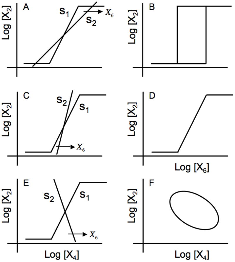
Graphical depiction of the steady-state solutions in the piecewise power-law representation. The panels on the left depict the open-loop transfer function from X₄ to X₂ is represented by the idealized sigmoid curve with maximum slope s₁ and that from X₂ to X₄ by the straight line with slope s₂ whose horizontal displacement is a function of the substrate concentration X₆. The panels on the right represent the corresponding steady-state induction characteristics produced by a slow increase in substrate concentration starting from a low value, followed by a slow decrease starting from a high value (top two panels) or phase portrait (bottom panel). (A) s₁ > s₂ > 0. (B) Discontinuous switching at different threshold values of X₆, depending on its history, produces bistability and hysteresis. (C) s₂ > s₁ > 0. (D) A continuous graded response for values of X₆ independent of its history. (E) s₁ > 0> s₂. (F) A stable limit-cycle depicting the trajectories of protein X₂ vs. inducer X₄ concentrations with time.

Note that the condition in Eqn. (17) is not satisfied independent of mechanistic detail for the specific architecture in the core model for the lactose system, as can be seen by substituting the values for the aggregate kinetic orders of the lactose system: g₂₁ = g₃₂ = g₅₂ = 1, g₁₄ = 2, and h₁₁ = h₂₂ = g₅₄ =1 [8, 9]. We will make extensive use of this condition for comparisons with the augmented models in Section 4.

By contrast, if s₂ > s₁ > 0 or s₁ > 0 > s₂

$$(g_{32}-g_{52})<\frac{h_{11}{h}_{22}{g}_{54}}{g_{21}{g}_{14}}$$ (18)

and there are three possibilities, depending on the signs of the penultimate Routh criterion [ $({\theta }_1{\theta }_2-{\theta }_3){\theta }_3-{\theta }_1^2{\theta }_4$] and the penultimate coefficient of the characteristic equation [θ₃].

3.3.2. Continuous graded induction

If $({\theta }_1{\theta }_2-{\theta }_3){\theta }_3-{\theta }_1^2{\theta }_4>0$, then

$$\frac{{\theta }_1}{2}\left[{\theta }_2-\sqrt{{\theta }_2^2-4{\theta }_4}\right]<{\theta }_3<\frac{{\theta }_1}{2}\left[{\theta }_2+\sqrt{{\theta }_2^2-4{\theta }_4}\right]$$ (19)

Under these conditions the system is locally stable. In this case there is only one steady-state solution, as can be seen in Fig. 4C for the case in which s₂ > s₁ > 0. This steady-state solution is always locally stable, regardless of whether the system is operating in the regulatable region, or at the maximal or basal rates of transcription. Thus, the steady-state induction characteristic manifests this by a continuous graded induction as shown in Fig. 4D. This behavior is what we expect for an inducible catabolic system based on a cost/benefit criterion [8, 9, 16]; the system will adjust the level of expression to match the availability of substrate in the organism’s environment. [Simulation of the model normalized to a steady state at the geometric mean between maximal and basal expression exhibits graded induction with the following values for the parameters: ρ=100, F₁ = 30, F₂ = 1, F₃ = F₄ = 300, g₁₄ = 2, h₁₁ = h₂₂ = g₂₁ = g₃₆ = g₅₄ = 1, g₃₂ = 1, g₄₂ = 1, g₅₂ = 0.4, and g₄₃ = 1 (data not shown)].

3.3.3. Limit cycle behavior

If $({\theta }_1{\theta }_2-{\theta }_3){\theta }_3-{\theta }_1^2{\theta }_4<0$ and ${\theta }_3>{\theta }_3^{\ast }$ (where the critical value ${\theta }_3^{\ast }<0$), then

$${\theta }_3^{\ast }<{\theta }_3<\frac{{\theta }_1}{2}\left[{\theta }_2-\sqrt{{\theta }_2^2-4{\theta }_4}\right]$$ (20)

Under these conditiions the system possesses complex conjugate eigenvalues with a positive real part. This possibility also exhibits only a single steady-state solution, as can be seen in Fig. 4E for the case in which s₁ > 0 > s₂ or

$$(g_{32}-g_{52})<0<\frac{h_{11}{h}_{22}{g}_{54}}{g_{21}{g}_{14}}$$

However, the steady-state solution in this case typically exhibits oscillatory instability. An unstable focus in a bounded region of state space (dictated by the maximal and basal limits on the rate of transcription) leads to limit cycle oscillations (Fig 4F).

For example, oscillations will be exhibited if ${\theta }_3>{\theta }_3^{\ast }$ and

$$(g_{42}-g_{52})>\frac{h_{11}{h}_{22}{g}_{54}}{g_{21}{g}_{14}}\left[1+\frac{F_3}{F_2}\frac{g_{43}}{h_{22}}+\frac{F_3}{F_1}\frac{g_{43}}{h_{11}}+\frac{F_3}{F_4}\frac{g_{43}}{g_{54}}\right]$$ (21)

while the condition in Eqn. (18) continues to hold. It should be noted that this set of conditions with realistic parameter values requires X₃ to nearly saturate the enzyme β-galactosidase, which is unlikely to be the case for the lactose system. [Simulation of the model normalized to a steady state at the geometric mean between maximal and basal expression exhibits limit-cycle oscillations with the following values for the parameters: ρ= 100, x₆ = 1, F₁ = 30, F₂ = 1, F₃ = F₄ = 300, g₁₄ = 2, h₁₁ = h₂₂ = g₂₁ = g₃₆ = g₅₄ = 1, g₃₂ = 0, g₄₂ = 1, g₅₂ = 0.1, and 0.000795< g₄₃ < 0.0015 (data not shown)].

3.3.4. Dysfunctional induction

If ${\theta }_3<{\theta }_3^{\ast }<0$, then the system possesses two positive-real eigenvalues. For example, if

$$(g_{42}-g_{52})\gg \frac{h_{11}{h}_{22}{g}_{54}}{g_{21}{g}_{14}}\left[1+\frac{F_3}{F_2}\frac{g_{43}}{h_{22}}+\frac{F_3}{F_1}\frac{g_{43}}{h_{11}}+\frac{F_3}{F_4}\frac{g_{43}}{g_{54}}\right]$$ (22)

while the condition in Eqn. (18) is satisfied, then the two eigenvalues are positive real but there is still only a single steady state that is unstable. It should be noted that this set of conditions requires β-galactosidase to be nearly saturated by its substrate, intracellular lactose (g₄₃ →0). This dysfunctional situation implies that intracellular lactose will either increase without bound, or decrease until the system eventually reverts to one of the generic cases described above. [Simulation of the model normalized to a steady state at the geometric mean between maximal and basal expression exhibits non-physiological variations in X₃ with the following values for the parameters: ρ = 100, x₆ = 1, F₁ = 30, F₂ = 1, F₃ = F₄ = 300, g₁₄ = 2, h₁₁ = h₂₂ = g₂₁ = g₃₆ = g₅₄ = 1, g₃₂ = 0, g₄₂ = 1, g₅₂ = 0.1, and 0 < g₄₃ < 0.000795 (data not shown)].

We can interpret these results in a different way that will facilitate comparisons with the results in Section 4. By expanding Eqn. (9) we can rewrite it as

$${\lambda }^5+{\phi }_1{\lambda }^4+{\phi }_2{\lambda }^3+{\phi }_3{\lambda }^2+{\phi }_4\lambda +{\phi }_5=0$$ (23)

$$\begin{array}{l}\text{with}{\phi }_1=F_1{h}_{11}+F_2{h}_{22}+F_3{g}_{43}+F_4{g}_{54}+F_5{g}_{75},\\ {\phi }_2=F_1{F}_2{h}_{11}{h}_{22}+F_1{F}_3{h}_{11}{g}_{43}+F_1{F}_4{h}_{11}{g}_{54}+F_1{F}_5{h}_{11}{g}_{75}+F_2{F}_3{h}_{22}{g}_{43}+F_2{F}_4{h}_{22}{g}_{54}+F_2{F}_5{h}_{22}{g}_{75}+F_3{F}_4{g}_{43}{g}_{54}+F_3{F}_5{g}_{43}{g}_{75}+F_4{F}_5{g}_{54}{g}_{75},\\ {\phi }_3=F_1{F}_2{F}_3{h}_{11}{h}_{22}{g}_{43}+F_1{F}_2{F}_3{F}_4[h_{11}{h}_{22}{g}_{54}-g_{21}{g}_{54}(g_{42}-g_{52})]+F_1{F}_2{F}_5{h}_{11}{h}_{22}{g}_{75}+F_1{F}_3{F}_4{h}_{11}{g}_{43}{g}_{54}+F_1{F}_3{F}_5{h}_{11}{g}_{43}{g}_{75}+F_1{F}_4{F}_5{h}_{11}{g}_{54}{g}_{75}+F_2{F}_3{F}_4{h}_{22}{g}_{43}{g}_{54},+F_2{F}_3{F}_5{h}_{22}{g}_{43}{g}_{75}+F_2{F}_4{F}_5{h}_{22}{g}_{54}{g}_{75}+F_3{F}_4{F}_5{g}_{43}{g}_{54}{g}_{75}\\ {\phi }_4=F_1{F}_2{F}_3{F}_4{g}_{43}[h_{11}{h}_{22}{g}_{54}-(g_{32}-g_{52})g_{21}{g}_{14}]+F_1{F}_2{F}_3{F}_5{h}_{11}{h}_{22}{g}_{43}{g}_{75}+F_1{F}_2{F}_4{F}_5{g}_{75}[h_{11}{h}_{22}{g}_{54}-(g_{42}-g_{52})g_{21}{g}_{14}]+F_1{F}_3{F}_4{F}_5{h}_{11}{g}_{43}{g}_{54}{g}_{75},\text{and}+F_2{F}_3{F}_4{F}_5{h}_{22}{g}_{43}{g}_{54}{g}_{75}\\ {\phi }_5=F_1{F}_2{F}_3{F}_4{F}_5{g}_{43}{g}_{75}[h_{11}{h}_{22}{g}_{54}-(g_{32}-g_{52})g_{21}{g}_{14}]\end{array}$$

The first two coefficients are obviously positive and the third is positive if

$$(g_{42}-g_{52})<\frac{h_{11}{h}_{22}{g}_{54}}{g_{21}{g}_{14}}\left[\begin{array}{l}1+\frac{F_3{g}_{43}}{F_1{h}_{11}}+\frac{F_3{g}_{43}}{F_2{h}_{22}}+\frac{F_3{g}_{43}}{F_4{g}_{54}}+\frac{F_5{g}_{75}}{F_1{h}_{11}}+\frac{F_5{g}_{75}}{F_2{h}_{22}}+\frac{F_5{g}_{75}}{F_4{g}_{54}}+\frac{F_3{F}_5{g}_{43}{g}_{75}}{F_1{F}_2{h}_{11}{h}_{22}}+\frac{F_3{F}_5{g}_{43}{g}_{75}}{F_1{F}_4{h}_{11}{g}_{54}}+\frac{F_3{F}_5{g}_{43}{g}_{75}}{F_2{F}_4{h}_{22}{g}_{54}}\end{array}\right]$$

This is always true for realistic parameter values, since the maximum for the left side is 1 (with g₄₂ = 1 and g₅₂ = 0 ) and the minimum for the right side is >25 (with h₁₁ = h₂₂ = g₅₄ = g₂₁ = g₇₅ = 1, g₁₄ =4, and the turnover time for the metabolite far from saturating its enzyme, F₅, approximately 100 times faster than that for the protein being diluted by exponential growth, F₂ ). The right side is much larger still if intracellular lactose is far from saturating β-galactosidase.

The corresponding Routh Criteria for stability can be expressed as follows:

$$\begin{array}{l}{R}_1={\phi }_1>0,R_2={\mathrm{\Delta }}_{21}=({\phi }_1{\phi }_2-{\phi }_3)/{\phi }_1>0,R_3=({\phi }_3{\mathrm{\Delta }}_{21}-{\phi }_1{\mathrm{\Delta }}_{22})/{\mathrm{\Delta }}_{21}>0(\text{where}\\ {\mathrm{\Delta }}_{22}=({\phi }_1{\phi }_4-{\phi }_5)/{\phi }_1),R_4=({\mathrm{\Delta }}_{22}{R}_3-{\phi }_5{R}_2)/R_3>0,\text{and}{R}_5={\phi }_5>0\end{array}$$

In the case of the core lactose system, it follows that the first three coefficients of the characteristic equation and the first three Routh criteria are always positive for the steady state in the regulatable region. On the other hand, all the coefficients of the characteristic equation and all of the Routh criteria are positive for the other two steady states.

In summary, the design of the core lactose system involves three considerations: the relative slopes of the transfer functions in the regulatable region, Descartes’ Rule of Signs, and the Routh Criteria for stability. These are all captured by the design principle in Eqn. (17), which is a necessary and sufficient condition for bistability. There are four characteristic behaviors determined by the nature of the steady state in the regulatable region.

Bistability is indicated by

• The relative slopes establishing the possibility of three steady states

• The last coefficient of the characteristic equation being negative whether the penultimate one is positive or negative, which establishes the existence of a single positive real eigenvalue

• The last Routh criterion being negative while the penultimate one is positive, again establishing one positive real eigenvalue for the characteristic equation

Under these conditions (R₄ > 0, φ₅ < 0) the system is dominated by positive feedback, with β-galactosidase having a greater influence on the production of the inducer allolactose than on its loss.

Monostability is indicated by

• The relative slopes establishing the possibility of a single steady state

• The last two coefficient of the characteristic equation being positive, establishing that there are no positive real eigenvalues

• The last two Routh criteria being positive, again establishing that there are no eigenvalues for the characteristic equation that have a positive real part

When the condition in Eqn. (17) is first violated (R₄ > 0, φ₅ = ε > 0), the core system becomes locally stable [Eqn. (20)]. The positive and negative feedbacks are now in a relative balance, with β-galactosidase having a comparable influence on the production and loss of inducer.

Limit Cycle Stability is indicated by

• The relative slopes establishing the possibility of a single steady state

• The last coefficient of the characteristic equation being positive while the penultimate one is positive or negative, establishing the existence of either zero or two positive real eigenvalues

• The last Routh criterion being positive while the penultimate one is negative, establishing complex conjugate eigenvalues of the characteristic equation with a positive real part when the system is near the bifurcation with the mononstable case

Reducing φ₄ (θ₃) [compare Eqns. (23) and (9)] with φ₅ > 0 eventually leads to a bifurcation that produces a stable limit cycle [Eqn. (21)] in the core system, and negative feedback dominates, with β-galactosidase having a greater influence on the loss of the inducer than on its production.

Dysfunctional Instability is indicated by

• The relative slopes establishing the possibility of a single steady state

• The last coefficient of the characteristic equation being positive while the penultimate one is positive or negative, establishing the existence of either zero or two positive real eigenvalues

• The last Routh criterion being positive while the penultimate one is negative, establishing two positive real eigenvalues of the characteristic equation when the system is far from the bifurcation with the mononstable case

Finally, with φ ₅ > 0 and a further reduction in φ ₄, beyond another critical value [Eqn. (22)], the core system becomes dysfunctional.

From all of the results in this section, we conclude that the condition in Eqn. (17) is both necessary and sufficient for bistability, and when it is not satisfied the core model exhibits locally stability, limit-cycle stability, or a dysfunctional instability.

4. Augmented models of the lac system

We and others have suggested mechanisms that might be capable of making lactose induction all-or-none. There are several mechanisms known to influence the expression of the lac system, and although they have been studied extensively in E. coli they are still not fully understood [45]. These include inducer exclusion [19], catabolite repression via the global regulator CRP [20], glucose transport [46], alternative fates for the intermediates [21–24], and growth-rate dependent dilution [26, 30]. Although one could attempt to model each of these mechanisms in detail, most models include the assumption of transfer functions between intracellular glucose (or some down-stream metabolite) and the rate of substrate transport or the rate of mRNA synthesis that are monotonic. For the purposes of determining the critical condition for instability of the steady state in the regulatable region it is essential that the key topological or architectural features and the signs of the interactions be represented faithfully. This will occur if the logarithmic gains between the inputs and outputs of the aggregated processes do not change sign.

The influence of the parameters for the individual processes within these aggregated processes will then appear in the logarithmic gain expressions, which in turn can be absorbed into an aggregate kinetic order parameter [16]. I will henceforth assume that each of the additional mechanisms involves a response to a downstream metabolic signal [glucose or some component of the phosphoenolpyruvate (PEP):carbohydrate phosphotransferase system (PTS)] represented by X₅.

4.1. Inducer exclusion

If we add inducer exclusion to the core model of the lactose system, as shown in Fig. 5, then the influence of X₅ on lactose uptake is given by the logarithmic gain L₃₅, which can be reinterpreted as an aggregate kinetic order g₃₅. The corresponding dynamic equations for the system in the regulatable region are the following:

$$\begin{array}{l}\frac{{dX}_1}{dt}={\alpha }_1{X}_0^{g_{10}}{X}_4^{g_{14}}-{\beta }_1{X}_1^{h_{11}}\\ \frac{{dX}_2}{dt}={\alpha }_2{X}_1^{g_{21}}-{\beta }_2{X}_2^{h_{22}}\\ \frac{{dX}_3}{dt}={\alpha }_3{X}_2^{g_{32}}{X}_5^{g_{35}}{X}_6^{g_{36}}-{\alpha }_4{X}_2^{g_{42}}{X}_3^{g_{43}}\\ \frac{{dX}_4}{dt}={\alpha }_4{X}_2^{g_{42}}{X}_3^{g_{43}}-{\alpha }_5{X}_2^{g_{52}}{X}_4^{g_{54}}\\ \frac{{dX}_5}{dt}={\gamma }_5{X}_2^{k_{52}}{X}_4^{k_{54}}{X}_{10}^{k_{5,10}}-{\alpha }_7{X}_5^{g_{75}}\end{array}$$ (24)

where

Fig. 5.

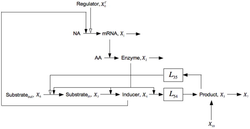
Expansion of the model in Fig. 1 that includes inducer exclusion, represented by the negative influence of X₅ on the import of X₆, and the uptake of extracellular glucose, represented by the pool X₁₀. This model allows for the possibility of several potential processes within the boxes that represent their aggregate behavior with the steady-state logarithmic gain indicated. See the legend of Fig. 1 and discussion in the text for details.

$$\begin{array}{l}{\gamma }_5{X}_2^{k_{52}}{X}_4^{k_{54}}{X}_{10}^{k_{5,10}}={\alpha }_5{X}_2^{g_{52}}{X}_2^{g_{54}}+{\beta }_{10}{X}_{10}^{h_{10,10}}\\ k_{52}=\frac{V_5}{V_5+V_{10}}{g}_{52}{k}_{54}=\frac{V_5}{V_5+V_{10}}{g}_{54}{k}_{5,10}=\frac{V_{10}}{V_5+V_{10}}{h}_{10,10}{V}_7=V_5+V_{10}\end{array}$$

and the V_k are the values of the fluxes into the k^th pool (or in the one exception, from the 10^th pool) at the steady state under consideration. Note that all the parameters in this case are positive except for g₃₅ < 0.

The steady-state equations are obtained by setting the derivative to zero, rearranging terms, and taking logarithms.

$$\begin{array}{l}-h_{11}{y}_1+g_{14}{y}_4=log({\beta }_1/{\alpha }_1)-g_{10}{y}_0\\ g_{21}{y}_1-h_{22}{y}_2=log({\beta }_2/{\alpha }_2)\\ (g_{32}-g_{42})y_2=g_{43}{y}_3+g_{35}{y}_5=log({\alpha }_4/{\alpha }_3)-g_{36}{y}_6\\ (g_{42}-g_{52})y_2+g_{43}{y}_3-g_{54}{y}_4=log({\alpha }_5/{\alpha }_4)\\ k_{52}{y}_2+k_{54}{y}_4-g_{75}{y}_5=log({\alpha }_7/{\gamma }_5)-k_{5,10}{y}_{10}\end{array}$$ (25)

The ‘open-loop’ transfer function form X₄ to X₂ has the same slope as that of the core model

$$s_1=g_{21}{g}_{14}/(h_{11}{h}_{22})$$

whereas that from X₂ to X₄ now has slope

$$s_2=(g_{54}{g}_{75}-g_{35}{k}_{54})/[k_{52}{g}_{35}+g_{75}(g_{32}-g_{52})]$$ (26)

The condition for bistability in this case is then

$$(g_{32}-g_{52})>\frac{h_{11}{h}_{22}{g}_{54}}{g_{21}{g}_{14}}\left[1+\left(\frac{k_{54}}{g_{54}}\right)\left(\frac{-g_{35}}{g_{75}}\right)\right]+k_{52}\left(\frac{-g_{35}}{g_{75}}\right)$$ (27)

Comparing this condition with that for bistability of the core model [Eqn. (17)], one sees that addition of inducer exclusion results in the right side being modified by a multiplicative factor greater than one and the addition of a positive term. Both have the effect of making it more difficult to satisfy the condition for bistability.

All of the behaviors described in Section 2 for the core model are exhibited in this case as well, under suitable conditions. In addition, there is a new possibility with inducer exclusion because the penultimate Routh criterion can now be negative for the basal and maximal steady states while all of the coefficients of the characteristic equation are positive, which indicates complex conjugate eigenvalues with a positive real part. This raises the possibility of limit-cycle oscillation around any steady state. This possibility can be understood intuitively as follows. At any fixed rate of transcription, the system is formally equivalent to a metabolic pathway subject to end-product inhibition [16]. Therefore it can display the same range of behaviors as such systems, including limit-cycle oscillations, although the cooperativity required is unrealistically large because of the short path length and the frequency is very high given the high turnover of the metabolic pools. [Simulation of the model normalized to a steady state at the geometric mean between maximal and basal expression exhibits limit-cycle oscillations with the following values for the parameters: ρ= 100, x₆ = 1, F₁ = 30, F₂ = 1, F₃ = F₄ = F₅ = 300, g₁₄ = 2, h₁₁ = h₂₂ = g₂₁ = g₃₆ = g₅₄ = g₇₅ = 1, g₃₂ = 1, g₄₂ = 1, g₅₂ = 0, g₄₃ = 1, and g₃₅ = −9. Under these same conditions, inducer exclusion converts the system exhibiting bistability to monostability when g₃₅ > − 8 (data not shown)].

Since the condition in Eqn. (17) is not satisfied for the core lactose system, adding inducer exclusion is incapable of making the induction all-or-none. The aggregate kinetic orders may vary with the mechanistic details and operating point, but the above result is mechanism independent and depends only on the architecture and signs of the interactions.

4.2. Catabolite repression

If we add catabolite repression to the core model of the lactose system, as shown in Fig. 6, then the influence of X₅ on the synthesis of lac mRNA X₁ is given by the logarithmic gain L₁₅, which can be reinterpreted as an aggregate kinetic order g₁₅. The resulting dynamic equations for the system are then the following:

$$\begin{array}{l}\frac{{dX}_1}{dt}={\alpha }_1{X}_0^{g_{10}}{X}_4^{g_{14}}{X}_5^{g_{15}}-{\beta }_1{X}_1^{h_{11}}\\ \frac{{dX}_2}{dt}={\alpha }_2{X}_1^{g_{21}}-{\beta }_2{X}_2^{h_{22}}\\ \frac{{dX}_3}{dt}={\alpha }_3{X}_2^{g_{32}}{X}_6^{g_{36}}-{\alpha }_4{X}_2^{g_{42}}{X}_3^{g_{43}}\\ \frac{{dX}_4}{dt}={\alpha }_4{X}_2^{g_{42}}{X}_3^{g_{43}}-{\alpha }_5{X}_2^{g_{52}}{X}_4^{g_{54}}\\ \frac{{dX}_5}{dt}={\gamma }_5{X}_2^{k_{52}}{X}_4^{k_{54}}{X}_{10}^{k_{5,10}}-{\alpha }_7{X}_5^{g_{75}}\end{array}$$ (28)

where

Fig. 6.

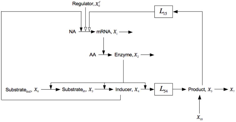
Expansion of the model in Fig. 1 that includes catabolite repression, represented by the negative influence of X₅ on the synthesis of lac mRNA X₁, and the uptake of extracellular glucose, represented by the pool X₁₀. See the legends of Figs. 1 and 5, and the discussion in the text for details.

$$\begin{array}{l}{\gamma }_5{X}_2^{k_{52}}{X}_4^{k_{54}}{X}_{10}^{k_{5,10}}={\alpha }_5{X}_2^{g_{52}}{X}_4^{g_{54}}+{\beta }_{10}{X}_{10}^{h_{10,10}}\\ k_{52}=\frac{V_5}{V_5+V_{10}}{g}_{52}{k}_{54}=\frac{V_5}{V_5+V_{10}}{g}_{54}{k}_{5,10}=\frac{V_{10}}{V_5+V_{10}}{h}_{10,10}{V}_7=V_5+V_{10}\end{array}$$

Note that all the parameters in this case are positive except for g₁₅ < 0.

The corresponding steady state equations are:

$$\begin{array}{l}-h_{11}{y}_1+g_{14}{y}_4+g_{15}{y}_5=log({\beta }_1/{\alpha }_1)-g_{10}{y}_0\\ g_{21}{y}_1-h_{22}{y}_2=log({\beta }_2/{\alpha }_2)\\ (g_{32}-g_{42})y_2-g_{43}{y}_3=log({\alpha }_4/{\alpha }_3)-g_{36}{y}_6\\ (g_{42}-g_{52})y_2+g_{43}{y}_3-g_{54}{y}_4=log({\alpha }_5/{\alpha }_4)\\ k_{52}{y}_2+k_{54}{y}_4-g_{75}{y}_5=log({\alpha }_7/{\gamma }_5)-k_{5,10}{y}_{10}\end{array}$$ (29)

The ‘open-loop’ transfer function form X₄ and X₅ to X₂ has slope

$$s_1=\frac{g_{21}{g}_{14}{k}_{52}{g}_{75}-g_{21}{k}_{52}{k}_{54}(-g_{15})}{k_{52}(h_{11}{h}_{22}{g}_{75}-g_{21}{k}_{52}{g}_{15})}$$ (30)

whereas that from X₂ to X₄ has the same slope as the core lactose model

$$s_2=g_{54}/(g_{32}-g_{52})$$ (31)

The condition for bistability in this case is

$$(g_{32}-g_{52})\left[1-\left(\frac{k_{54}}{g_{14}}\right)\left(\frac{-g_{15}}{g_{75}}\right)\right]>\frac{h_{11}{h}_{22}{g}_{54}}{g_{21}{g}_{14}}\left[1+\left(\frac{g_{21}{k}_{52}}{h_{11}{h}_{22}}\right)\left(\frac{-g_{15}}{g_{75}}\right)\right]$$ (32)

Comparing this condition with that for bistability of the core model [Eqn. (17)], one sees that catabolite repression results in the left side being modified by a multiplicative factor less than one and the right side being modified by a multiplicative factor greater than one. Both have the effect of making it more difficult to satisfy the condition for bistability.

All of the behaviors described in Section 4.1 for the model with inducer exclusion are exhibited in this case as well, under suitable conditions. Moreover, there is another new possibility because in this case only the first two Routh criteria are guaranteed to be positive. When the third and the fifth Routh criteria are negative, Descartes’ Rule shows that there is only one positive real eigenvalue. Thus, there are complex conjugate eigenvalues with a positive real part and one positive real eigenvalue. This raises the hypothetical possibility of bistability with oscillations around the maximal steady state. This possibility can be understood intuitively as follows. Once inducer has dissociated the repressor from its operator sites, the system is formally equivalent to an amino acid biosynthetic gene circuit subject to repression by the end-product co-repressor [16]. Thus it can hypothetically display the same range of behaviors as such systems, including limit-cycle oscillations, although the difference in time scales between protein and metabolite concentrations means that the effective path length is kinetically shortened making this even less likely than is the case with inducer exclusion. [Simulation of the model normalized to a steady state at the geometric mean between maximal and basal expression converts the system exhibiting bistability to monostability with the following values for the parameters: ρ= 100, x₆ = 1, F₁ = 30, F₂ = 1, F₃ = F₄ = F₅ = 300, g₁₄ = 2, h₁₁ = h₂₂ = g₂₁ = g₃₆ = g₅₄ = g₇₅ = 1, g₃₂ = 1, g₄₂ = 1, g₅₂ = 0, g₄₃ = 1, and g₁₅ = −0.7. However, even with unrealistically high values for the cooperativity (g₁₅ < −8) the system with catabolite repression remains stable (data not shown)].

Since the condition in Eqn. (17) is not satisfied for the core lactose system, adding catabolite repression is incapable of making the induction all-or-none and this result is independent of the mechanistic details.

4.3. Alternative fates for intermediates

If we add an alternative fate for each of the intermediates X₃ and X₄ in the core lactose model, represented as alternative processes leading to X₈ and X₉ in Fig. 7, then the resulting S-system equations in the regulatable region are the following:

$$\begin{array}{l}\frac{{dX}_1}{dt}={\alpha }_1{X}_0^{g_{10}}{X}_4^{g_{14}}-{\beta }_1{X}_1^{h_{11}}\\ \frac{{dX}_2}{dt}={\alpha }_2{X}_1^{g_{21}}-{\beta }_2{X}_2^{h_{22}}\\ \frac{{dX}_3}{dt}={\alpha }_3{X}_2^{g_{32}}{X}_6^{g_{36}}-{\delta }_3{X}_2^{f_{32}}{X}_3^{f_{33}}\\ \frac{{dX}_4}{dt}={\alpha }_4{X}_2^{g_{42}}{X}_3^{g_{43}}-{\delta }_4{X}_2^{f_{42}}{X}_4^{f_{44}}\\ \frac{{dX}_5}{dt}={\alpha }_5{X}_2^{g_{52}}{X}_4^{g_{54}}-{\alpha }_7{X}_5^{g_{75}}\end{array}$$ (33)

where

Fig. 7.

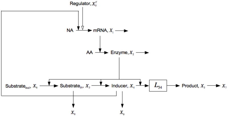
Expansion of the model in Fig. 1 that includes non-inducible processes creating alternative fates for the intermediates. For X₃ the alternative fate is its loss to X₈ and for X₄ it is its loss to X₉. See the legends of Figs. 1 and 5, and the discussion in the text for details.

$$\begin{array}{l}{\delta }_3{X}_2^{f_{32}}{X}_3^{f_{33}}={\alpha }_4{X}_2^{g_{42}}{X}_3^{g_{43}}+{\alpha }_8{X}_3^{g_{83}}\\ f_{33}=\frac{V_4}{V_3}{g}_{43}+\frac{V_8}{V_3}{g}_{83}{f}_{32}=\frac{V_4}{V_3}{g}_{42}{V}_4=V_3-V_8\end{array}$$

$$\begin{array}{l}{\delta }_4{X}_2^{f_{42}}{X}_4^{f_{44}}{X}_5^{f_{45}}={\alpha }_5{X}_2^{g_{52}}{X}_4^{g_{54}}+{\alpha }_9{X}_4^{g_{94}}\\ f_{44}=\frac{V_5}{V_4}{g}_{54}+\frac{V_9}{V_4}{g}_{94}{f}_{42}=\frac{V_5}{V_4}{g}_{52}{V}_5=V_4-V_9\end{array}$$

Note that all the parameters in this case are positive.

The steady-state equations are the following:

$$\begin{array}{l}-h_{11}{y}_1+g_{14}{y}_4=log({\beta }_1/{\alpha }_1)-g_{10}{y}_0\\ g_{21}{y}_1-h_{22}{y}_2=log({\beta }_2/{\alpha }_2)\\ (g_{32}-f_{32})y_2-f_{33}{y}_3=log({\delta }_3/{\alpha }_3)-g_{36}{y}_6\\ (g_{42}-f_{42})y_2+g_{43}{y}_3-f_{44}{y}_4=log({\delta }_4/{\alpha }_4)\\ g_{52}{y}_2+g_{54}{y}_4-g_{75}{y}_5=log({\alpha }_7/{\alpha }_5)\end{array}$$ (34)

The ‘open-loop’ transfer function form X₄ to X₂ has the same slope as for the core model

$$s_1=g_{21}{g}_{14}/(h_{11}{h}_{22})$$

whereas that from X₂ to X₄ now has slope

$$s_2=f_{33}{f}_{44}/[g_{43}(g_{32}-f_{32})+f_{33}(g_{42}-f_{42})]$$ (35)

The condition for bistability in this case is:

$$\left(\frac{g_{43}}{f_{33}}\right)(g_{32}-f_{32})+(g_{42}-f_{42})>\frac{h_{11}{h}_{22}{g}_{54}}{g_{21}{g}_{14}}\left(\frac{f_{44}}{g_{54}}\right)$$ (36)

Comparing this condition with that for bistability of the core model [Eqn. (17)], one finds that the left side is typically made larger. This can be seen most easily by making use of the relationships following Eqn. (33) and noting that f₃₃ and f₄₄ are each weighted averages between two processes assumed to be first order; the above condition then becomes:

$$(g_{32}-g_{52})+\left[\frac{V_8}{V_3}{g}_{42}+\frac{V_9}{V_4}{g}_{52}\right]>\frac{h_{11}{h}_{22}{g}_{54}}{g_{21}{g}_{14}}$$ (37)

Thus, the addition of alternative flux V₈ or V₉, or both, only adds to the left side, thus making it easier to satisfy the condition for bistability [16, 17, 29, 40].

The range of behaviors described in Section 4.1 for the model with inducer exclusion are exhibited in this case as well, under similar conditions according to Descartes’ Rule applied to the characteristic equation and Routh’s Criteria for stability. However, in this case, as noted above, it is easier to satisfy the condition for bistability.

It should be emphasized that this mechanism independent interpretation only applies if the alternative fate is not coordinately inducible with β-galactosidase, as this would imply a different topology for the model. If it were, then there would be no difference in the aggregate kinetic orders for production and removal of inducer. In fact, if the removal of gratuitous inducer were coordinately inducible with the lac permease, then models of the lac system would not account for the experimental results of Novick and Weiner [11]. Similarly, it must be established whether or not the export of intermediates [21–24] is coordinately inducible with the lac genes. If not, then the above interpretation of the simple design principle is legitimate and there is the possibility of bistability; but if they were induced in parallel, then the condition could not be satisfied and then monostability would be indicated. Nuances in the interpretation of aggregate kinetic orders have not always been understood; hence, I will return to this critical issue in the Discussion (Section 7).

4.4. Growth-rate dependent dilution

If we consider cellular growth rate to be a function of nutrient status, which is related to X₅ and can be enhanced by the influx of exogenous glucose X₁₀, then adding growth-rate dependent dilution to each of the pools in the core lactose model means including X₅ in one of their loss functions. For mRNA this is represented by the additional loss to X₁₁, for the enzymes this is loss to X₁₂ (dilution by growth is the only loss for stable proteins), for intercellular lactose this is loss to X₁₃, for inducer this is loss to X₁₄, and for product this is loss to X₁₅ (Fig. 8). Although alternative fates for intermediate pools were the focus in Section 4.3, the alternatives in this case are specifically a function of growth rate. The resulting equations in this case are the following:

$$\begin{array}{l}\frac{{dX}_1}{dt}={\alpha }_1{X}_0^{g_{10}}{X}_4^{g_{14}}-{\delta }_1{X}_1^{f_{11}}{X}_5^{f_{15}}\\ \frac{{dX}_2}{dt}={\alpha }_2{X}_1^{g_{21}}-{\delta }_2{X}_2^{f_{22}}{X}_5^{f_{25}}\\ \frac{{dX}_3}{dt}={\alpha }_3{X}_2^{g_{32}}{X}_6^{g_{36}}-{\delta }_3{X}_2^{f_{32}}{X}_3^{f_{33}}{X}_5^{f_{35}}\\ \frac{{dX}_4}{dt}={\alpha }_4{X}_2^{g_{42}}{X}_3^{g_{43}}-{\delta }_4{X}_2^{f_{42}}{X}_4^{f_{44}}{X}_5^{f_{45}}\\ \frac{{dX}_5}{dt}={\gamma }_5{X}_2^{k_{52}}{X}_4^{k_{54}}{X}_5^{k_{55}}{X}_{10}^{k_{5,10}}-{\delta }_5{X}_5^{f_{55}}\end{array}$$ (38)

where

Fig. 8.

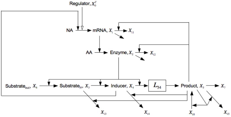
Expansion of the model in Fig. 1 that includes growth-rate dependent dilution of pools represented by an alternative fate that is positively influenced by X₅ (proportional to flux of carbon). The alternative fates in this case are represented as fluxes to the dummy variables X₁₁, X₁₂, X₁₃, X₁₄, and X₁₅. See the legends of Figs. 1 and 5, and the discussion in the text for details.

$$\begin{array}{l}{\delta }_1{X}_1^{f_{11}}{X}_5^{f_{15}}={\beta }_1{X}_1^{h_{11}}+{\alpha }_{11}{X}_1^{g_{11,1}}{X}_5^{g_{11,5}}\\ f_{11}=\frac{(V_1-V_{11})}{V_1}{h}_{11}+\frac{V_{11}}{V_1}{g}_{11,1}=1f_{15}=\frac{V_{11}}{V_1}{g}_{11,5}=\frac{V_{11}}{V_1}{g}_{75}\end{array}$$

$$\begin{array}{l}{\delta }_2{X}_2^{f_{22}}{X}_5^{f_{25}}={\beta }_2{X}_2^{h_{22}}+{\alpha }_{12}{X}_2^{g_{12,2}}{X}_5^{g_{12,5}}\\ f_{22}=\frac{(V_2-V_{12})}{V_2}{h}_{22}+\frac{V_{12}}{V_2}{g}_{12,2}=1f_{25}=\frac{V_{12}}{V_2}{g}_{12,5}=\frac{V_{12}}{V_2}{g}_{75}\end{array}$$

$$\begin{array}{l}{\delta }_3{X}_2^{f_{32}}{X}_3^{f_{33}}{X}_5^{f_{35}}={\alpha }_4{X}_2^{g_{42}}{X}_3^{g_{43}}+{\alpha }_{13}{X}_3^{g_{13,3}}{X}_5^{g_{13,5}}\\ f_{33}=\frac{V_4}{V_3}{g}_{43}+\frac{V_{13}}{V_3}{g}_{13,3}{f}_{32}=\frac{V_4}{V_3}{g}_{42}{f}_{35}=\frac{V_{13}}{V_3}{g}_{13,5}=\frac{V_{13}}{V_3}{g}_{75}{V}_4=V_3-V_{13}\end{array}$$

$$\begin{array}{l}{\delta }_4{X}_2^{f_{42}}{X}_4^{f_{44}}{X}_5^{f_{45}}={\alpha }_5{X}_2^{g_{52}}{X}_4^{g_{54}}+{\alpha }_{14}{X}_4^{g_{14,4}}{X}_5^{g_{14,5}}\\ f_{44}=\frac{V_5}{V_4}{g}_{54}+\frac{V_{14}}{V_4}{g}_{14,4}{f}_{42}=\frac{V_5}{V_4}{g}_{52}{f}_{45}=\frac{V_{14}}{V_4}{g}_{14,5}=\frac{V_{14}}{V_4}{g}_{75}{V}_5=V_4-V_{14}\end{array}$$

$$\begin{array}{l}{\gamma }_5{X}_2^{k_{52}}{X}_4^{k_{54}}{X}_5^{k_{55}}{X}_{10}^{k_{5,10}}={\alpha }_5{X}_2^{g_{52}}{X}_4^{g_{54}}+{\beta }_{10}{X}_5^{h_{10,5}}{X}_{10}^{h_{10,10}}\\ k_{52}=\frac{V_5}{V_5+V_{10}}{g}_{52}{k}_{54}=\frac{V_5}{V_5+V_{10}}{g}_{54}{k}_{55}=\frac{V_{10}}{V_5+V_{10}}{h}_{10,5}=\frac{V_{10}}{V_5+V_{10}}{g}_{75}{k}_{5,10}=\frac{V_{10}}{V_5+V_{10}}{h}_{10,10}\end{array}$$

$$\begin{array}{l}{\delta }_5{X}_5^{f_{55}}={\beta }_5{X}_5^{h_{55}}+{\alpha }_7{X}_5^{g_{75}}\\ f_{55}=g_{75}+\frac{V_{15}}{V_7+V_{15}}{V}_7=V_5+V_{10}-V_{15}\end{array}$$

Note that all the parameters in this case are positive and that

$$(f_{55}-k_{55})=\frac{V_5}{V_5+V_{10}}{g}_{75}+\frac{V_{15}}{V_7+V_{15}}>0$$

The steady-state equations are the following:

$$\begin{array}{l}-f_{11}{y}_1+g_{14}{y}_4-f_{15}{y}_5=log({\delta }_1/{\alpha }_1)-g_{10}{y}_0\\ g_{21}{y}_1-f_{22}{y}_2-f_{25}{y}_5=log({\delta }_2/{\alpha }_2)\\ (g_{32}-f_{32})y_2-f_{33}{y}_3-f_{35}{y}_5=log({\delta }_3/{\alpha }_3)-g_{36}{y}_6\\ (g_{42}-f_{42})y_2+g_{43}{y}_3-f_{44}{y}_4-f_{45}{y}_5=log({\delta }_4/{\alpha }_4)\\ k_{52}{y}_2+k_{54}{y}_4-(f_{55}-k_{55})y_5=log({\delta }_5/{\gamma }_5)-k_{5,10}{y}_{10}\end{array}$$ (39)

The condition for bistability in this case is:

$$\left[\left(\frac{g_{43}}{f_{33}}\right)(g_{32}-f_{32})+(g_{42}-f_{42})\right]\left\{1-\frac{k_{54}\left[g_{21}{f}_{15}+h_{11}\left(\frac{f_{11}}{h_{11}}\right)f_{25}\right]}{g_{21}{g}_{14}(f_{55}-k_{55})}\right\}>\frac{h_{11}{h}_{22}{g}_{54}}{g_{21}{g}_{14}}\left(\frac{f_{11}}{h_{11}}\right)\left(\frac{f_{22}}{h_{22}}\right)\left(\frac{f_{44}}{g_{54}}\right)+\frac{k_{52}{f}_{44}\left[g_{21}{f}_{15}+h_{11}\left(\frac{f_{11}}{h_{11}}\right)f_{25}\right]}{g_{21}{g}_{14}(f_{55}-k_{55})}+\frac{\left[g_{21}{k}_{52}{g}_{14}+h_{11}{h}_{22}\left(\frac{f_{11}}{h_{11}}\right)\left(\frac{f_{22}}{h_{22}}\right)k_{54}\right]\left(\left(\frac{g_{43}}{f_{33}}\right)f_{35}+f_{45}\right)}{g_{21}{g}_{14}(f_{55}-k_{55})}$$ (40)

By making use of the relationships following Eqn. (38), and noting that f₁₁, f₂₂, f₃₃ and f₄₄ are each weighted averages between two processes assumed to be first order, this condition becomes:

$$\left[(g_{32}-g_{52})+\left(\frac{V_8}{V_3}{g}_{42}+\frac{V_9}{V_4}{g}_{52}\right)\right]\left\{1-\frac{k_{54}[g_{21}{f}_{15}+h_{11}{f}_{25}]}{g_{21}{g}_{14}(f_{55}-k_{55})}\right\}>\frac{h_{11}{h}_{22}{g}_{54}}{g_{21}{g}_{14}}+\frac{k_{52}{f}_{44}[g_{21}{f}_{15}+h_{11}{f}_{25}]}{g_{21}{g}_{14}(f_{55}-k_{55})}+\frac{[g_{21}{k}_{52}{g}_{14}+h_{11}{h}_{22}{k}_{54}](f_{35}+f_{45})}{g_{21}{g}_{14}(f_{55}-k_{55})}$$ (41)

Comparing this condition with that for bistability of the core model [Eqn. (17)], one sees that the losses from the X₁ through X₄ pools by growth-dependent dilution (terms involving f₁₅, f₂₅, f₃₅, and f₄₅ ) result in the left side being modified by a multiplicative factor less than one and the right side by the addition of positive terms, all of which have the effect of making it more difficult to satisfy the condition for bistability. The loss from the X₅ pool by growth-dependent dilution (terms involving f₅₅ ) diminishes the effect of the losses from these other pools but it still leaves the net stabilizing result unchanged. On the other hand, losses from the X₃ and X₄ pools by growth-dependent dilution (terms involving V₈ and V₉ ) add to the left side, thus promoting the instability necessary for the induction to be all-or-none, as was seen in Section 4.3. All of these effects are relatively small, as will be seen in the Discussion (Section 7).

The range of behaviors described in Section 4.2 for the model with catabolite repression are exhibited in this case as well, under similar conditions according to Descartes’ Rule applied to the characteristic equation and Routh’s Criteria for stability. However, in this case, as noted above, it is more difficult to satisfy the condition for bistability in most cases; losses from the X₃ and X₄ pools are the exception, as also shown in Section 4.3.

All of the additions to the core lac model considered in this section make it more difficult to generate an all-or-none induction, except for the addition of alternative fates for intermediates. Thus, it is the non-inducible alternative fate for the natural inducer that is critical for generating an hysteretic response [17, 29, 40]. By having an alternative fate that is not part of the inducible response, the aggregate kinetic order for the influence of the inducible proteins on the degradation of the inducer, g₅₂, is made less than the influence of the inducible proteins on the synthesis of the inducer, g₃₂. This allows the positive feedback to dominate over the negative feedbacks. However, for this to be significant, the flux to the alternative fate must be relatively large, which is unlikely the case when the alternative fate is simply dilution by exponential growth [17, 40]. All of the other mechanisms essentially provide additional negative feedback, making it more difficult to generate the dominant positive feedback necessary for exponential instability.

5. A system design principle

As noted in the introduction, the core model of the lactose system has a simple design principle [43]; namely,

$$(g_{32}-g_{52})>\frac{h_{11}{h}_{22}{g}_{54}}{g_{21}{g}_{14}}\text{for}\text{a}\text{discontinuous}\text{hysteretic}\text{switch}$$ (42)

that is able to account for several well-known experiments with the lactose system when one assumes minimal alternative fates for intermediates, such as dilution by exponential growth. As will be seen in Section 6, this same design principle applies to the more general case with larger fluxes to the alternative fate, although the interpretation of the aggregate kinetic orders changes.

5.1. Sadler and Novick (1965)

The core model accounts for the classic experimental results of Sadler and Novick [47] in which they observed a continuous graded induction without hysteresis. In their experiments they used a mutant strain of E. coli in which the lac permease was inactivated (g₃₂ = 0 ) and they induced the lac operon with a gratuitous inducer isopropyl-β-D-1-thiogalactoside (IPTG). In this system, the inducer is not acted upon by any part of the inducible pathway (g₄₂ = g₅₂ = 0 ), and if one assumes non-inducible influx and efflux then the extracellular and intracellular concentrations of inducer are proportional. This is an open-loop system in which expression of the operon is simply proportional to the rate of transcription as determined by the steady-state concentration of intracellular IPTG, which is proportional to the concentration of extracellular IPTG (Fig. 9A). When the values of the parameters for the lactose system (g₁₄ = 2 and g₂₁ = h₁₁ = h₂₂ = g₅₄ = 1 [8, 9]) are substituted into the design principle in Eqn. (42) one finds

Fig. 9.

Model of the inducible lactose system with various alterations in design. (A) The open-loop configuration. (B) A single positive feedback configuration. (C) A single negative feedback configuration. (D) The wild-type configuration with both positive and negative feedback loops. Note that the graphical representations are simplified for purposes of illustration; see the legend of Fig. 1 and discussion in the text for details.

$$(0-0)=0<\frac{1}{2}$$

and the prediction of a continuous graded induction is in agreement with the experimental evidence.

5.2. Novick and Weiner (1957)

The model also accounts for the classic experimental results of Novick and Weiner [11] in which they observed a discontinuous all-or-none switch with hysteresis. They induced the lac operon with a gratuitous inducer that was transported into the cell by the inducible Lac permease (g₃₂ = 1), was diluted by exponential growth, and was not acted upon by the remainder of the inducible pathway (g₄₂ = g₅₂ = 0 ). Hence, the gratuitous inducer occupied the position of immediate product for the inducible pathway (in this case simply the Lac permease step); hence, there is a simple positive feedback loop as depicted in Fig. 9B. When the values of the parameters for the lactose system are substituted into the design principle in Eqn. (42) one finds

$$(1-0)=1>\frac{1}{2}$$

and the prediction of a discontinuous hysteretic switch is in agreement with the experimental evidence. [If there were a major export of gratuitous inducer that was inducible along with the lac permease, then this condition would not be satisfied (as noted in Section 4.3).]

5.3. Prediction for substrate inducer

The design principle in Eqn. (42) makes two other predictions, which are related to the position of the natural inducer in the inducible pathway, that have yet to be tested experimentally. If one were to construct a mutant lacking an inducible transport system (g₃₂ = 0) for the natural inducer allolactose, which bypasses the first activity of β-galactosidase (g₄₂ = 0 ) and is catabolized by the second (g₅₂ = 1), then the position of the inducer would be that of the immediate substrate of the inducible system, as depicted in Fig. 9C. The design principle in this case would show

$$(0-1)=-1<\frac{1}{2}$$

and the prediction would be a graded induction, or (less likely) stable limit cycle or dysfunctional behavior.

5.4. Prediction for the natural lac system

More importantly, in the case of the natural lactose system, the substrate lactose is transported into the cell by the inducible permease, converted into the natural inducer allolactose by the action of the inducible enzyme β-galactosidase (g₃₂ = g₄₂ = 1), and the inducer also is degraded by the same inducible enzyme β-galactosidase (g₅₂ = 1). If one again assumes that the intermediates have negligible alternative fates, then the inducer is an intermediate in the inducible system (Fig. 9D). In this case, the design principle shows that

$$(1-1)=0<\frac{1}{2}$$

and the prediction is for a continuous graded induction. [Here we assumed limited dilution by growth, but this result would also apply to the possibility of a substantial but coordinately inducible alternative fate.]

The design principle has a simple interpretation for the case in which there might in fact be a non-inducible alternative fate for the inducer. It can be expressed as

$$(g_{32}-f_{42})>\frac{h_{11}{h}_{22}{g}_{54}}{g_{21}{g}_{14}}$$ (43)

The left side varies between 0 and 1, depending on the fraction of flux through the inducer pool being diverted to the alternative fate (V₉/V₅, with the largest fraction occurring at the basal level of gene expression), whereas the right side varies as the inverse of the effective cooperativity. An alternative representation of this condition for bistability is the following

$$1-\frac{1}{1+(V_9/V_5)}>\frac{1}{g_{14}}=\frac{1}{2}$$ (44)

when one takes into account the parameter values of the lac system and the definition of the aggregate kinetic order f₄₂ ; namely, g₂₁ = h₁₁ = h₂₂ = g₅₄ = 1, g₁₄ = 2, g₃₂ = g₄₂ = g₅₂ = 1, and f₄₂ = g₅₂V₅/(V₅ + V₉ ).

The fact that the core model of the lac operon predicts a continuous graded induction in response to extracellular lactose led to a search for relevant experimental data in the literature. We were unable to find any experimental evidence for either a continuous graded induction or a discontinuous hysteretic switch in response to lactose, which comes as a surprise. In experiments that one might have expected to find a discontinuous hysteretic induction if it were to exist, Ozbudak et al [41] found no evidence at the single cell level to support this expectation. This is in contrast to the Novick and Weiner [11] experiments in which a well-defined hysteresis can be seen even in mass culture.

6. System design space

To illustrate the analysis from the perspective of another global representation (the recast representation) within the power-law formalism, and to provide another view of the design principle, we will characterize the core lac model in system design space. For this purpose we will expand the mechanistic detail of the model in Fig. 1 to include a rational function description of transcription and a first-order, non-inducible loss of the inducer to the alternative fate represented by X₉.

6.1. Conventional sigmoid model

The conventional rational-function description of transcription [41, 48] involves n molecules of inducer binding cooperatively to the repressor and inducer-free repressor binding to an operator site to produce an hyperbolic inhibition of transcription. In the case of the lactose repressor, the reversible binding of n = 2 molecules of inducer X₄ to the free regulatory protein X₀ yields a complex C:

$$X_0+2X_4\ddot{\text{A}}C$$

At equilibrium, $X_4^2{X}_0=K_4^{2}C$, where the constant K₄ represents the concentration of inducer that binds half the total regulator, and the total concentration of regulator $X_0^T$ is the sum of both its free and bound forms, $X_0^T=X_0+C$. Solving these two equations for the concentration of free regulator yields

$$X_0=\frac{X_0^T}{1+{(X_4/K_4)}^2}$$ (45)

If one assumes that the free regulator binds to a single lac operator site with equilibrium dissociation constant K₁, then the rate of lac mRNA synthesis can be expressed as

$$V_1={\alpha }_{1M}\frac{1+{(X_4/K_4)}^2}{\rho +{(X_4/K_4)}^2}$$ (46)

where $\rho ={\alpha }_{1M}/{\alpha }_{1B}=1+(X_0^T/K_1)$ is the capacity for regulated expression.

If the rate law for the alternative fate of inducer is represented explicitly as ${\alpha }_9{X}_4^{g_{94}}$ and the variables are normalized as follows

$$\begin{array}{l}{x}_1=\frac{{\beta }_1}{{\alpha }_{1M}}{X}_1,x_2=\frac{{\beta }_1{\beta }_2}{{\alpha }_{1M}{\alpha }_2}{X}_2,x_3=\frac{{\alpha }_4}{{\alpha }_5{K}_4}{X}_3,x_4=\frac{1}{K_4}{X}_4,x_6=\frac{{\alpha }_3}{{\alpha }_5{K}_4}{X}_6\text{and}\\ \kappa =\frac{{\beta }_1{\beta }_2}{{\alpha }_{1B}{\alpha }_2{\alpha }_5}{\alpha }_9\end{array}$$ (47)

where κ can be considered the normalized rate constant for the alternative fate, then we can write the normalized dynamic equations for the model in Fig. 1 as

$$\begin{array}{l}\frac{1}{{\beta }_1}\frac{{dx}_1}{dt}=\frac{1+x_4^2}{\rho +x_4^2}-x_1\\ \frac{1}{{\beta }_2}\frac{{dx}_2}{dt}=x_1-x_2\\ \frac{{\alpha }_5\kappa }{{\alpha }_4{\alpha }_9}\frac{{dx}_3}{dt}=\rho x_2{x}_6-\rho x_2{x}_3\\ \frac{\kappa }{{\alpha }_9}\frac{{dx}_4}{dt}=\rho x_2{x}_3-\rho x_2{x}_4-\kappa x_4\end{array}$$ (48)

Note that h₁₁, h₂₂, g₅₄, g₂₁, g₃₂, g₄₂ and g₅₂ are all first-order in the lac system [8] and, for simplicity, we are assuming that g₄₃ = g₉₄ = 1 and that X₆ can represent any monotonic function of extracellular substrate. Moreover, the effective cooperativity of transcription g₁₄ = ∂logV₁/∂log X₄ varies from 0, through some maximum (≈2 ), and back to 0 as the inducer concentration increases from 0.

6.1.1. Recasting the steady-state equations

Setting the derivatives in Eqns. (48) to zero yields

$$\begin{array}{l}0=\frac{1+x_4^2}{\rho +x_4^2}-x_1\\ 0=x_1-x_2\\ 0=x_6-x_3\\ 0=\rho x_2{x}_3-\rho x_2{x}_4-\kappa x_4\end{array}$$ (49)

These equations can be recast in a number of ways into the generalized mass action representation within the power-law formalism, in this case simply by the introduction of a new variable $x_5=\rho +x_4^2$[31]. The resulting set of equations

$$0=x_5^{-1}+x_4^2{x}_5^{-1}-x_1$$ (50)

$$0=x_1-x_2$$ (51)

$$0=x_6-x_3$$ (52)

$$0=\rho x_2{x}_3-\rho x_2{x}_4-\kappa x_4$$ (53)

$$0=\rho +x_4^2-x_5$$ (54)

is mathematically equivalent to Eqns. (49). [Note that here x₅ is an auxiliary variable in the recast equations and is not related to the product concentration X₅ used in earlier sections.]

The composition of the recast equations is summarized by the system signature [36] {P₁, N₁, P₂, N₂, P₃, N₃, L, P_n, N_n}, in which P_i, and N_i are the number of positive and negative terms in the i^th equation and n is the number of equations. In this case, the system signature is {2,1,1,1,1,1,1,2,2,1}.

6.1.2. Selecting dominant terms in the GMA equations

We select a dominant positive and negative term from each equation and assign a term signature[36], [p₁, n₁, p₂, n₂, p₃, n₃, p₄, n₄, L, p_n, n_n] in which the numbers p_i and n_i indicate the order of the dominant terms in the i^th equation, and an associated case number.

If one were to select all combinations of dominant terms from each side of Eqns. (50) to (54), there would be 8 possible combinations: Case 1 [1,1,1,1,1,1,1,1,1,1], Case 2 [1,1,1,1,1,1,1,1,2,1], Case 3 [1,1,1,1,1,1,1,2,1,1], Case 4 [1,1,1,1,1,1,1,2,2,1], Case 5 [2,1,1,1,1,1,1,1,1,1], Case 6 [2,1,1,1,1,1,1,1,2,1], Case 7 [2,1,1,1,1,1,1,2,1,1], and Case 8 [2,1,1,1,1,1,1,2,2,1]. However, the two cases involving the first positive term of Eqn. (50) and the second positive term of Eqn. (54) [Case 2 and Case 4] will be invalid because they would imply that $x_4^2<1$ and $x_4^2>\rho >1$, which is impossible. For each of the remaining 6 cases, the analysis involves the same steps: identifying the S-system equations, determining the corresponding dominance conditions, solving the linear system of equations and inequalities to determine the boundaries of the valid solutions. This process will be illustrated for a representative case.

6.1.3. Calculation for Case 5 [2,1,1,1,1,1,1,1,1,1]

Picking the second positive term in Eqn. (50), the first negative term in Eqn. (53), and the first positive term in Eqn. (54) gives

$$\begin{array}{l}0=x_4^2{x}_5^{-1}-x_1\\ 0=x_1-x_2\\ 0=x_6-x_3\\ 0=x_2{x}_3-x_2{x}_4\\ 0=\rho -x_5\end{array}$$

which has the steady-state solution

$$x_1=\frac{x_6^2}{\rho }{x}_2=\frac{x_6^2}{\rho }{x}_3=x_6{x}_4=x_6$$

The dominance conditions that correspond to this set of equations are

$$1<x_3=x_4\kappa <\rho x_2{\rho }^{1/2}>x_3=x_4$$

Inserting the steady-state solution into the dominance conditions yields the boundaries within which the solution is valid.

$$1<x_6<{\rho }^{1/2}\kappa <x_6^2$$

6.1.4. Constructing system design space

An informative view of the system design space is obtained by plotting in normalized form (v₅/v₉ )_B = α₅ x_2B/α₉ = 1/κ, which is the ratio of primary flux to alternative flux at the basal steady state, as a function of x₆, which is the input concentration. The results are shown in Fig. 10, where the numbering of the regions corresponds to the valid cases.

Fig. 10.

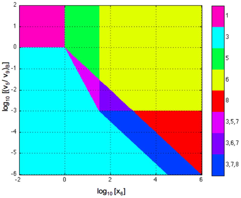
System design space for the conventional sigmoid model in Section 6.1. Ratio of primary to alternative flux at the basal steady state as a function of normalized input concentration. Stable steady states with the basal rate of transcription (Regions 1 and 3). Stable steady states with the maximal rate of transcription (Regions 6 and 8). Stable steady state with intermediate rates of transcription (Region 5). Unstable steady state with intermediate rates of transcription that lead to hysteresis (Region 7). The parameters in this case are n = 2 and ρ = 1000.

For other examples of system design spaces see [31–35, 49,50], and for details of the Design Space Toolbox in Matlab that automates the construction of the system design space see [36].

6.1.5. Comparison with bifurcation analysis

Although there are some similarities between system design space and conventional bifurcation diagrams, they are not the same. System design space has boundaries, which represent qualitatively distinct changes in phenotypic behavior that are not found in bifurcation diagrams. Moreover, the boundaries that do represent bifurcations in system design space are only approximately located. A comparison of the results from conventional bifurcation analysis with those generated in the construction of the system design space (Fig. 11) illustrates the magnitude of the quantitative difference.

Fig. 11.

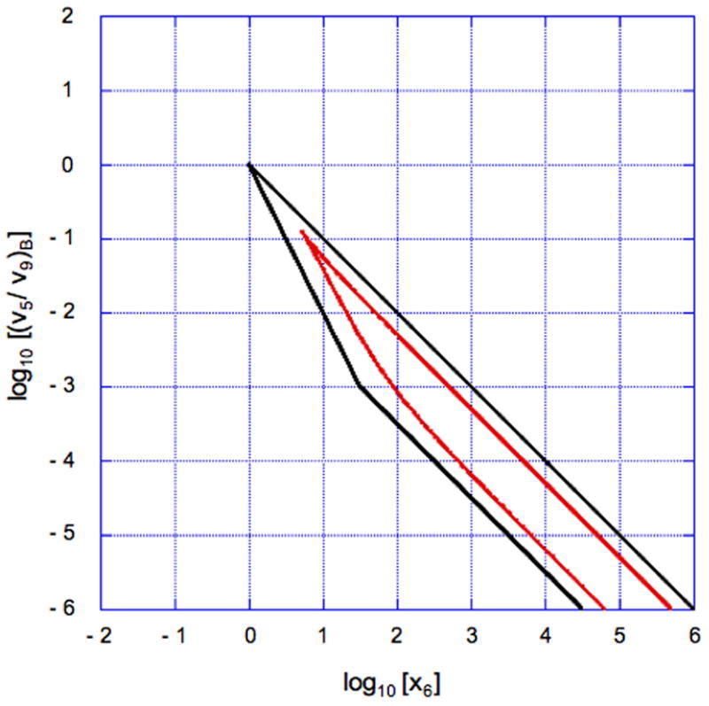
Accuracy of the hysteretic region in system design space. The boundaries of the hysteretic region determined by conventional bifurcation analysis are shown in red. The corresponding boundaries generated in the construction of the system design space are shown in black (Fig. 10). The overall shape of the hysteretic region is the same, but the extent of the region is overestimated by the boundaries in the system design space. The parameters in this comparison are n = 2 and ρ = 1000.

The essential features are the same, but the region representing hysteretic behavior is overestimated by the boundaries in the system design space. This is to be expected since the locations of the boundaries correspond to breakpoints determined by the assumption of dominance. It should be emphasized that the goal in constructing the system design space is not to faithfully represent the quantitatively exact behavior, but rather to capture the qualitatively distinct behaviors, which it manages to do very efficiently in ways that bifurcation analysis does not. Nevertheless, it should be noted that systems with more complex bifurcation patterns have yet to be explored.

6.2. Looped DNA model

The detailed molecular interactions in the lac system have undergone a major change with the recognition that the auxiliary operator sites play a key role in the regulation of lac expression [27, 51]. As a consequence of DNA looping repressor can cooperatively bind at two operator sides. In this section I construct the system design space for this model and compare it to the system design space of the older model in Section 6.1.

The reversible binding of inducer X₄ to one of the two sites on the regulatory protein (a dimer of dimers), X₀, is all that is needed to inactivate the repressor [28]. This binding can be represented as follows, where the bound form of the regulator is represented as a complex C

$$X_0+X_4\ddot{\text{A}}C$$

At equilibrium, X₄ X₀ = K₄C, where the equilibrium dissociation constant K₄ represents the concentration of inducer that binds half the total regulator, and the total concentration of regulator $X_0^T$ is the sum of both its free and bound forms, $X_0^T=X_0+C$. Solving these two equations for the concentration of free regulator yields

$$X_0=\frac{X_0^T}{1+(X_4/K_4)}$$ (55)

Note the difference from Eqn. (45).

In a similar fashion, if we assume binding of free repressor at three lac operator sites in the DNA and a cooperative interaction between any two via DNA looping [27], then the total DNA, D^T, will be distributed among several forms:

$$D^T=D\left[1+\frac{X_0}{K_A}+\frac{X_0}{K_B}+\frac{X_0}{K_C}+{\left(\frac{X_0}{K_{AB}}\right)}^2+{\left(\frac{X_0}{K_{AC}}\right)}^2+{\left(\frac{X_0}{K_{BC}}\right)}^2\right]$$

This can be simplified because the single binding at auxiliary sites B and C is negligible compared to that at the primary site A [27].

$$D^T=D\left[1+\frac{X_0}{K_A}+{\left(\frac{X_0}{K_{AB}}\right)}^2+{\left(\frac{X_0}{K_{AC}}\right)}^2+{\left(\frac{X_0}{K_{BC}}\right)}^2\right]$$

Assuming that transcription only occurs when the primary operator site A is free, we can write

$$V_1=\frac{D^T\left[1+{\left(\frac{X_0}{K_{BC}}\right)}^2\right]}{\left[1+\frac{X_0}{K_A}+{\left(\frac{X_0}{K_{AB}}\right)}^2+{\left(\frac{X_0}{K_{AC}}\right)}^2+{\left(\frac{X_0}{K_{BC}}\right)}^2\right]}$$ (56)

Letting the maximum rate constant for transcriptionα_1M be proportional to D^T, combining Eqns. (55) and (56), and simplifying yields the following expression for the rate of mRNA synthesis

$$V_1={\alpha }_{1M}\frac{\phi +2(X_4/K_4)+{(X_4/K_4)}^2}{\rho \phi +(2+\theta )(X_4/K_4)+{(X_4/K_4)}^2}$$ (57)

where $\phi =\left[1+{\left(\frac{X_0^T}{K_{BC}}\right)}^2\right],\theta =\frac{X_0^T}{K_A}$ and $\rho =\left[\phi +\theta +{\left(\frac{X_0^T}{K_{AB}}\right)}^2+{\left(\frac{X_0^T}{K_{AC}}\right)}^2\right]$, the capacity for regulated expression. More complete and quantitative molecular models could be examined, but this version will be sufficient for our qualitative analysis.

Finally, if the variables are normalized as in Eqns. (47) and the alternative fate for the inducer is represented explicitly, then we can write the normalized dynamic equations for the model in Fig. 1 as

$$\begin{array}{l}\frac{1}{{\beta }_1}\frac{{dx}_1}{dt}=\frac{\phi +2x_4+x_4^2}{\rho \phi +(2+\theta )x_4+x_4^2}-x_1\\ \frac{1}{{\beta }_2}\frac{{dx}_2}{dt}=x_1-x_2\\ \frac{{\alpha }_5\kappa }{{\alpha }_4{\alpha }_9}\frac{{dx}_3}{dt}=\rho x_2{x}_6-\rho x_2{x}_3\\ \frac{\kappa }{{\alpha }_9}\frac{{dx}_4}{dt}=\rho x_2{x}_3-\rho x_2{x}_4-\kappa x_4\end{array}$$ (58)

6.2.1. Recasting the steady-state equations

Setting the derivatives in Eqns. (58) to zero results in the following equations:

$$\begin{array}{l}0=\frac{\phi +2x_4+x_4^2}{\rho \phi +(2+\theta )x_4+x_4^2}-x_1\\ 0=x_1-x_2\\ 0=x_6-x_3\\ 0=\rho x_2{x}_3-\rho x_2{x}_4-\kappa x_4\end{array}$$ (59)

These equations can be recast into the generalized mass action representation within the power-law formalism by the introduction of the new variable $x_5=\rho \phi +(2+\theta )x_4+x_4^2$. The resulting set of equations

$$0=\phi x_5^{-1}+2x_4{x}_5^{-1}+x_4^2{x}_5^{-1}-x_1$$ (60)

$$0=x_1-x_2$$ (61)

$$0=x_6-x_3$$ (62)

$$0=\rho x_2{x}_3-\rho x_2{x}_4-\kappa x_4$$ (63)

$$0=\rho \phi +(2+\theta )x_4+x_4^2-x_5$$ (64)

is mathematically equivalent to Eqns. (59). In this case, the system signature is {3,1,1,1,1,1,1,2,3,1}.

6.2.2. Selecting dominant terms in the GMA equations

If one were to select all combinations of dominant terms from each equation there would be 18 possible cases. Again, not all combinations are valid. For example, the combinations involving the second positive term of Eqn. (60) and the third positive term of Eqn. (64) will be invalid because it would imply that x₄ < 2 and x₄ > (2 + θ)> 2, which is impossible. For each of the remaining cases, the analysis involves the same steps: identifying the S-system equations, determining the corresponding dominance conditions, solving the linear system of equations and inequalities to determine the boundaries of the valid solutions. This process will be illustrated for a representative case.

6.2.3. Calculation for Case 13 [3,1,1,1,1,1,1,1,1,1]

Case 13 (following an extension of the numbering system indicated in Section 6.1.2) is selected because it is somewhat analogous to Case 5 in the older model. Picking the third positive term in Eqn. (60), the first negative term in Eqn. (63), and the first positive term in Eqn. (64) to be dominant gives the following S-system

$$\begin{array}{l}0=x_4^2{x}_5^{-1}-x_1\\ 0=x_1-x_2\\ 0=x_6-x_3\\ 0=x_2{x}_3-x_2{x}_4\\ 0=\rho \phi -x_5\end{array}$$

which has the steady-state solution

$$x_1=\frac{x_6^2}{\rho \phi }{x}_2=\frac{x_6^2}{\rho \phi }{x}_3=x_4=x_6$$

The five dominance conditions for this case are

$$x_3=x_4>\sqrt{\phi }{x}_3=x_4>2\kappa <\rho x_2{x}_3=x_4<\frac{\rho \phi }{(2+\theta )}{x}_3=x_4<\sqrt{\rho \phi }$$

Inserting the steady-state solution into the dominance conditions yields the boundaries within which the solution is valid.

$$min\left\{\sqrt{\rho \phi },\frac{\rho \phi }{(2+\theta )}\right\}>x_6>max\{2,\sqrt{\phi }\}\kappa <\frac{x_6^2}{\phi }$$

6.2.4. Constructing system design space

The system design space is obtained by plotting in normalized form (v₅/v₉)_B = 1/κ, the ratio of primary flux to alternative flux at the basal steady state, as a function of x₆, the input concentration. The results are shown in Fig. 12, where the numbering of the regions corresponds to the valid cases.

Fig. 12.

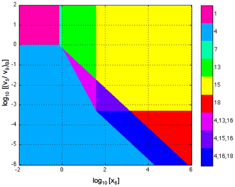
System design space for the looped DNA model in Section 6.2. Ratio of primary to alternative flux at the basal steady state as a function of normalized input concentration. Stable steady states with the basal rate of transcription (Regions 1 and 4). Stable steady states with the maximal rate of transcription (Regions 15 and 18). Stable steady states with intermediate rates of transcription (Region 7 and 13). Unstable steady state with intermediate rates of transcription that lead to hysteresis (Region 16). The parameters in this case are n = 2, ρ = 1000, θ = 18, and φ = 1.4.

6.3. Comparisons in system design space

A comparison of the system design space for the model in Section 6.2 (Fig. 12) with that for the model in Section 6.1 (Fig. 10) shows similarities and differences. Overall the geometry is similar with regions of stable steady states and hysteretic regions. However, the looped DNA model has an additional phenotypic region (Region 7), and the landmarks involve parameters with different physical meaning. In particular, for the model of Section 6.1, $\rho =1+\frac{X_0^T}{K_1}\approx \frac{X_0^T}{K_1}$, and doubling the concentration of total repressor leads to an approximate doubling of ρ, the capacity for regulation. Whereas, for the model of Section 6.2, $\rho =1+\frac{X_0^T}{K_A}+{\left(\frac{X_0^T}{K_{BC}}\right)}^2+{\left(\frac{X_0^T}{K_{AB}}\right)}^2+{\left(\frac{X_0^T}{K_{AC}}\right)}^2\approx {\left(\frac{X_0^T}{K_{AB}}\right)}^2+{\left(\frac{X_0^T}{K_{AC}}\right)}^2$, and doubling the concentration of total repressor leads to an approximate quadrupling of ρ.

The simple design principle in Section 5 can be reinterpreted in light of the conditions for bistability, as revealed in the system design space for the model in Section 6.1. Fig. 10 shows that the fraction of basal flux through the inducer pool that is diverted to the alternative fate must be sufficiently greater than that to the primary fate [Eqns. (44)], which can be expressed as

$${\left(\frac{V_9}{V_5}\right)}_B=\frac{{\alpha }_9}{{\alpha }_5{X}_{20B}}>\frac{1}{g_{14}-1}=1$$ (65)

This shows that the effective cooperativity g₁₄ must be greater than 1. As the quasi-steady state induction proceeds, and the steady-state level of enzyme X₂₀ increases, the fraction of alternative flux will only decrease, thus making it even more difficult to maintain bistability. As the total amount of repressor decreases, the basal level of expression increases (ρ decreases), making the basal fraction of alternative flux smaller and again reducing the potential for bistability. This can be expressed as

$${\left(\frac{V_9}{V_5}\right)}_B=\frac{{\alpha }_9{\beta }_1{\beta }_2}{{\alpha }_{1B}{\alpha }_2{\alpha }_5}=\frac{{\alpha }_9{\beta }_1{\beta }_2}{{\alpha }_2{\alpha }_5{\alpha }_{1M}}\left[1+\frac{X_0^T}{K_1}\right]>\frac{1}{g_{14}-1}=1$$ (66)

Thus, there are several factors that can promote bistability: (a) increasing the effective cooperativity, g₁₄, (b) increasing the rate constant for the alternative fate, α₉, (c) decreasing the rate constant for the primary fate of inducer, α₅, (d) increasing the rate constants for the turnover of lac mRNA, β₁, and enzymes, β₂, (e) decreasing the rate constants for lac basal transcription, α_1B, and for translation of lac mRNA, α₂, (f) increasing the total amount of constitutive repressor, $X_0^T$, and (g) decreasing the equilibrium dissociation constant for inducer binding to repressor, K₁.

For the model in Section 6.2, the results in Fig. 12 show that the new region, Case 7, corresponds to a region in which the effective cooperativity g₁₄ = 1 (i.e., no cooperativity). Thus, there is no hysteresis for the corresponding values of x₆. In addition, the upper limit for hysteresis is shifted to lower values of the flux ratio (v₅/v₉)_B. Thus, a higher value of basal flux to the alternative fate is required to achieve bistability. This can be seen in the reinterpretation of the design principle in Section 5. For values of x₆ with an effective cooperativity g₁₄ ≈ n = 1 (Case 7), the condition for bistability

$${\left(\frac{V_9}{V_5}\right)}_B=\frac{{\alpha }_9{\beta }_1{\beta }_2}{{\alpha }_{1B}{\alpha }_2{\alpha }_5}=\frac{{\alpha }_9{\beta }_1{\beta }_2}{{\alpha }_2{\alpha }_5{\alpha }_{1M}}\left[1+\frac{X_0^T}{K_A}+{\left(\frac{X_0^T}{K_{BC}}\right)}^2+{\left(\frac{X_0^T}{K_{AB}}\right)}^2+{\left(\frac{X_0^T}{K_{AC}}\right)}^2\right]>\infty$$

cannot be satisfied. Only when the value of x₆ increases and crosses the boundary between regions 7 and 13 is an effective cooperativity g₁₄ ≈ n = 2 established, and the condition for bistability

$${\left(\frac{V_9}{V_5}\right)}_B=\frac{{\alpha }_9{\beta }_1{\beta }_2}{{\alpha }_{1B}{\alpha }_2{\alpha }_5}=\frac{{\alpha }_9{\beta }_1{\beta }_2}{{\alpha }_2{\alpha }_5{\alpha }_{1M}}\left[1+\frac{X_0^T}{K_A}+{\left(\frac{X_0^T}{K_{BC}}\right)}^2+{\left(\frac{X_0^T}{K_{AB}}\right)}^2+{\left(\frac{X_0^T}{K_{AC}}\right)}^2\right]>1$$

can be satisfied for sufficiently large values of the alternative to primary flux ratio.

From these comparisons of the different models for the lac system one can see that it may be even more difficult to achieve bistability with the looped DNA model than with the conventional model that is no longer accepted.

7. Discussion

The classic experiments of Novick and Weiner [11] demonstrated that the lac system of E. coli could exhibit an all-or-none hysteretic response to the artificial situation in which the gratuitous inducer TMG is taken up by the inducible permease but not metabolized by the cell. This remarkable paper has had a major impact on the field of gene regulation, as evident by its frequent and continuous citation over the years. However, many if not most of these citations interpret the hysteretic response as a property of the lac system responding to its natural inducer, which is metabolized by the cell.

The experiments of Novick and Weiner [11] have recently been repeated at the single cell level [41] and interpreted as evidence of multistability of the natural system. However, when the natural substrate lactose rather than the artificial inducer TMG was used there appeared to be no evidence of multistability. Ozbudak et al also used multiple-copy plasmids to provide extra copies of lac operator DNA so as to reduce the available repressor by titration. When the titration reached a critical level, as predicted by an approximate 20-fold reduction in the capacity for regulation, the hysteretic response was converted to a graded response.

Since their prediction was based on the conventional sigmoid model (Section 6.1), the 20-fold reduction in capacity for regulation would suggest the equivalent reduction in the effective concentration of repressor. However, if these results are interpreted in terms of the looped DNA model (Section 6.2), then the suggested reduction in effective repressor concentration need only be approximately 4 fold (Section 6.3).

The mathematical models that have attempted to account for bistability in the lac system have gotten more detailed over the years but have not clarified our understanding. There are still claims for and against bistability in the natural system, based mostly on mathematical considerations rather than biological ones and confounded by the lack of any definitive biological experiments.

Our own models also have incorporated more details of the lac system, and at each stage we have made predictions regarding bistability. Although the conditions vary in detail as the models have become more complex, the key condition for bistability has not changed and can be expressed most efficiently in terms of the aggregate kinetic orders whose reinterpretation accounts for the added complexity of the models. In our case, we come down on the side of monostability. The reasons have to do with biological considerations as well as mathematical analysis.

There are four biological reasons that have influenced our conclusions. First, when placed in the larger biological context of inducible catabolic systems, lac along with other members of this general class exhibit overall design features predicted on the basis of monostability [8, 9]. Both the molecular mode of control (repressor or activator) and coupling of regulator and effector functions (directly coupled, uncoupled or inversely coupled) have been predicted for this class of systems and there are now abundant examples of experimental results that confirm these predictions [10].

Second, evolutionary cost/benefit considerations, which were a part of the criteria used to make well-controlled comparisons for this class of systems [16], argue against bistability. The argument is straightforward. There will be a threshold value of substrate that must be exceeded before induction of the catabolic machinery will benefit the cell. This is to be expected whether the system is bistable or monostable. Now consider a monostable system at a stable steady state in the middle of its expression range with substrate in the middle of its effective range. A small increase in substrate will lead to a correspondingly small increase in lac expression, and conversely a small decrease will lead to a small deinduction. This makes reasonable physiological sense. Contrast this behavior with that expected of a bistable system. Again assume a steady state, in this case unstable, in the middle of its expression range with substrate in the middle of its effective range. A small increase in substrate would lead to full induction of the system; the ~ 30-fold excess in protein synthesis would be a significant cost to the cell. In contrast, a small decrease in substrate would lead to the complete deinduction of the system and thus a failure to utilize the available suprathreshold levels of substrate. In either bistable case, there is a physiological mismatch between the environment and the cellular response. van Hoek and Hogeweg [29] also have incorporated such evolutionary cost/benefit considerations into their simulations and come to the same conclusion favoring monostability for the lac system.

Third, in rigorously controlled comparisons of switching time for bistable and monostable systems, bistable systems were found to be slower [18], which would leave them at a disadvantage in the highly variable environments experienced by E. coli [52]. This difference in switching time also is reported to play a role in the simulations favoring the evolution of monostability [29].

Finally, there is the lack of experimental data to support a prediction of bistability. Despite the long history of study involving the lac operon, such experiments apparently have not been reported. The reason undoubtedly has to do with the difficulty in performing the experiment rigorously in mass culture. One must grow cells in very dilute culture so that their utilization of lactose during the experiment does not significantly change the concentration in the environment; this means that there will be little material available for the assay of enzymatic activity. Also, the cells must be grown for a least 4 to 5 generations in each of the different concentrations of lactose so that a steady state is established. These conditions are analogous to those required for a steady-state enzyme kinetic measurement; the enzyme concentration must be low enough so that the substrate concentration is not changed significantly during the period of the assay and this results in a small amount of product for measurement [53]. On the other hand, in the exquisite single-cell studies of Taniguchi et al [42], quantifying on the genome-scale levels of mRNA and protein in E. coli, they “did not observe clear bimodal distributions among 1018 strains [genes] under their growth conditions, which indicates that bimodal distributions are generally rare”. Although they did not subject the cells to a wide variety of grow conditions, their conclusion is convincing because they observed large fluctuations in expression that could conceivably establish the conditions for bimodal expression in some cells if the mechanisms for its generations existed.

Our mathematical models have suggested a biological design principle, which is most efficiently expressed in terms of aggregate kinetic orders (Section 5), that elucidates the key qualitative features of the system that could lead to bistability. These features are (a) the difference between the aggregate kinetic orders with respect to the catalysts (transporters and enzymes) for production and removal of inducer (g₃₂ − g₅₂ ), (b) the aggregate kinetic order representing the effective cooperativity of the inducers effect on transcription (g₁₄ ), (c) the aggregate kinetic order for loss of inducer ( h₃₃ ), and (d) the aggregate kinetic orders comprising the open-loop transfer function from lac mRNA to the induced proteins (h₁₁h₂₂/g₂₁ ). There are kinetic data available to estimate most of these features [8, 9]. The aggregate kinetic order for the production of inducer with respect to a change in the permease and β-galactosidase is 1 (g₃₂ = 1), whereas the maximum aggregate kinetic order for the removal of inducer with respect to a change in the β-galactosidase is 1 (0 < g₅₂ < 1), when the ratio of primary to alternative flux is maximum. The maximum effective cooperativity is 2 (0 ≤ g₁₄ ≤ 2) depending upon the concentration of inducer. The effective loss of inducer is first order (g₅₄ = 1), assuming that a first-order process represents the alternative flux. The transfer function from lac mRNA to levels of β-galactosidase is linear (g₂₁ = h₁₁ = h₂₂ = 1).

For the core model, the right side of Eqn. (43) is determined essentially by the inverse of the maximum effective cooperativity, and in Eqn. (44) it is given a typical value of ½. Thus, the key issue is the difference on the left side of Eqn. (43), which is determined by the ratio of alternate V₉ to primary V₅ fluxes [Eqn. (44)]. Moreover, the critical condition is when this ratio is near one, thus lowering the value of the aggregate kinetic order f₄₂ to 1/2. It seems clear that this condition would not be met if the alternative flux were simply dilution by exponential growth. An underestimate of the primary flux is ~ 2 fg/min [54] if one ignores the carbon lost to CO₂ and secreted products; an overestimate of the loss by dilution is ~ 0.2 fg/min if one assumes that the intracellular allolactose concentration is near its K_M value for β-galactosidase when the experimental evidence suggests a value much less [8]. Such estimates indicate that the alternative flux would be less than 0.1 of the primary flux. Thus, the core model of the lac system is expected to be monostable.

Augmenting the core model to include several other mechanisms simply makes it more difficult to achieve bistability [Eqns. (27), (32), and (41)]. Only a major efflux of intermediates, equivalent to the primary flux to products, that is not coordinately induced with lac operon expression could make it easier to satisfy the condition for bistability [Eqn. (37)].

The design principle, as seen from the perspective of the system design space, reveals a relationship among several factors that are capable of promoting bistability (Section 6.3). When the results for the conventional model of lac transcription (Fig. 10) are compared with those for the looped-DNA model (Fig. 12), one sees that an extra region of design space is introduced making it more difficult to achieve bistability. A comparison of the hysteretic region obtained from the construction of the system design space with that obtained from conventional bifurcation analysis (Fig. 11) shows that the design space overestimates the hysteretic region, as expected from the analogy [16] to traditional Bode plots [55]. The overestimate should not be a surprise if one recalls that the intended purpose of systems design space analysis is to provide an efficient means of uncovering the essential qualitative features of a system design rather than a detailed quantitative analysis of the system under consideration. There could be values of parameters that would lead to bistability when the qualitative analysis predicts monostability, or alternatively that would lead to monostability when the prediction is bistability. However, the differences are not expected to be great. If this is seen as a disadvantage, then it needs to be contrasted with the advantages of the qualitative analysis. One can carry out the analysis and construct the system design space much more efficiently than one could do an exhaustive quantitative analysis including a complete bifurcation analysis. Moreover, an exhaustive analysis of parameter space would be an inefficient means to obtain the regions of qualitatively distinct behavior, which are identified with ease in the system design space; even for a moderately sized model, the exploration of parameter space becomes a combinatorial explosion of simulations, which ultimately limits the scope of such an analysis.

In light of the above biological considerations and modeling predictions, we continue to come down on the side of the lac system being monostable. However, confirmatory experimental studies are still lacking. More complete models might provide precise quantitative conditions if all the requisite experimental data were available. Lacking these, our models and conclusions are most useful for simply capturing the essential qualitative results. The proposed design principle in Section 5 provides the simplest statement of these conclusions.

References

- 1.Jacob F, Monod J. Genetic regulatory mechanisms in the synthesis of proteins. J Mol Biol. 1961;3:318–356. doi: 10.1016/s0022-2836(61)80072-7. [DOI] [PubMed] [Google Scholar]
- 2.Beckwith JR, Zipser D, editors. The Lactose Operon. Cold Spring Harbor Laboratory; Cold Spring Harbor, New York: 1970. [Google Scholar]
- 3.Miller JH, Reznikoff WS, editors. The Operon. Cold Spring Harbor Laboratory; Cold Spring Harbor, New York: 1980. [Google Scholar]
- 4.Müller-Hill B. The Lac Operon: A Short History of a Genetic Paradigm. Walter de Gruyter; Berlin: 1996. [Google Scholar]
- 5.Savageau MA. Genetic regulatory mechanisms and the ecological niche of Escherichia coli. Proc Nat Acad Sci USA. 1974;71:2453–2455. doi: 10.1073/pnas.71.6.2453. [DOI] [PMC free article] [PubMed] [Google Scholar]
- 6.Savageau MA. Are there rules governing patterns of gene regulation? In: Goodwin BC, Saunders PT, editors. Theoretical Biology -- Epigenetic and Evolutionary Order. Edinburgh University Press; Edinburgh: 1989. pp. 42–66. [Google Scholar]
- 7.Shinar G, Dekel E, Tlusty T, Alon U. Rules for biological regulation based on error minimization. Proc Natl Acad Sci USA. 2006;103:3999–4004. doi: 10.1073/pnas.0506610103. [DOI] [PMC free article] [PubMed] [Google Scholar]
- 8.Hlavacek WS, Savageau MA. Subunit structure of regulator proteins influences the design of gene circuitry: Analysis of perfectly coupled and completely uncoupled circuits. J Mol Biol. 1995;248:739–755. doi: 10.1006/jmbi.1995.0257. [DOI] [PubMed] [Google Scholar]
- 9.Hlavacek WS, Savageau MA. Rules for coupled expression of regulator and effector genes in inducible circuits. J Mol Biol. 1996;255:121–139. doi: 10.1006/jmbi.1996.0011. [DOI] [PubMed] [Google Scholar]
- 10.Wall ME, Hlavacek WS, Savageau MA. Design of gene circuits: Lessons from bacteria. Nature Reviews Genetics. 2004;5:34–42. doi: 10.1038/nrg1244. [DOI] [PubMed] [Google Scholar]
- 11.Novick A, Weiner M. Enzyme induction as an all-or-none phenomenon. Proc Natl Acad Sci USA. 1957;43:553–566. doi: 10.1073/pnas.43.7.553. [DOI] [PMC free article] [PubMed] [Google Scholar]
- 12.Griffith JS. Mathematics of cellular control processes II. Positive feedback to one gene. J Theoret Biol. 1968;20:209–216. doi: 10.1016/0022-5193(68)90190-2. [DOI] [PubMed] [Google Scholar]
- 13.Babloyantz A, Sanglier M. Chemical instabilities of “all-or-none” type in β-galactosidase induction and active transport. FEBS Lett. 1972;23:364–366. doi: 10.1016/0014-5793(72)80317-x. [DOI] [PubMed] [Google Scholar]
- 14.Sanglier M, Nicolis G. Sustained oscillations and threshold phenomena in an operon control circuit. Biophysical Chem. 1976;4:113–121. doi: 10.1016/0301-4622(76)85001-6. [DOI] [PubMed] [Google Scholar]
- 15.Jobe A, Bourgeois S. lac repressor-operator interaction. VI. The natural inducer of the lac operon. J Mol Biol. 1972;69:397–408. doi: 10.1016/0022-2836(72)90253-7. [DOI] [PubMed] [Google Scholar]
- 16.Savageau MA. Biochemical Systems Analysis: A Study of Function and Design in Molecular Biology. (40) http://www.amazon.com/Biochemical-Systems-Analysis-Function-Molecular/dp/1449590764/ 2009 a reprinting of the original edition published by Addison-Wesley, Reading, Mass., 1976.]
- 17.Savageau MA. Design of gene circuitry by natural selection: Analysis of the lactose catabolic system in E. coli. Biochem Soc Trans. 1999;27:264–270. doi: 10.1042/bst0270264. [DOI] [PubMed] [Google Scholar]
- 18.Savageau MA. Alternative designs for a genetic switch: Analysis of switching times using the piece-wise power-law representation. Math Biosci. 2002;180:237–253. doi: 10.1016/s0025-5564(02)00113-x. [DOI] [PubMed] [Google Scholar]
- 19.Deutscher J, Franke C, Postma PW. How phosphotransferase system-related protein phosphorylation regulates carbohydrate metabolism in bacteria. Microbiol Mol Biol Rev. 2006;70:939–1031. doi: 10.1128/MMBR.00024-06. [DOI] [PMC free article] [PubMed] [Google Scholar]
- 20.Park YH, Lee RR, Seok Y-J, Peterkofsky A. In vitro reconstitution of catabolite repression in Escherichia coli. J Biol Chem. 2006;281:6448–6454. doi: 10.1074/jbc.M512672200. [DOI] [PubMed] [Google Scholar]
- 21.Huber RE, Kurz G, Wallenfels K. A quantitation of the factors which affect the hydrolase and transgalactosylase activities of β-galactosidase (E. coli) on lactose. Biochemistry. 1976;15:1994–2001. doi: 10.1021/bi00654a029. [DOI] [PubMed] [Google Scholar]
- 22.Huber RE, Hurlburt KL. Escherichia coli growth on lactose requires cycling of β-galactosidase products into the medium. Can J Microbiol. 1984;30:411–418. doi: 10.1139/m84-060. [DOI] [PubMed] [Google Scholar]
- 23.Liu JY, Miller PF, Gosink M, Olson ER. The identification of a new family of sugar efflux pumps in Escherichia coli. Mol Microbiol. 1999;31:1845–1851. doi: 10.1046/j.1365-2958.1999.01321.x. [DOI] [PubMed] [Google Scholar]
- 24.Liu JY, Miller PF, Willard J, Olson ER. Functional and biochemical characterization of Escherichia coli sugar efflux transporters. J Biol Chem. 1999;274:22977–22984. doi: 10.1074/jbc.274.33.22977. [DOI] [PubMed] [Google Scholar]
- 25.Chung JD, Stephanopoulos G. On physiological multiplicity and population heterogeneity of biological systems. Chem Eng Sci. 1996;51:1509–1521. [Google Scholar]
- 26.Narang A, Pilyugin SS. Bistability of the lac operon during growth of Escherichia coli on lactose and lactose+glucose. Bull Math Biol. 2008;70:1032–1064. doi: 10.1007/s11538-007-9289-7. [DOI] [PubMed] [Google Scholar]
- 27.Oehler S, Eismann ER, Krämer JH, Müller-Hill B. The three operators of the lac operon cooperate in repression. EMBO J. 1990;9:973–979. doi: 10.1002/j.1460-2075.1990.tb08199.x. [DOI] [PMC free article] [PubMed] [Google Scholar]
- 28.Oehler S, Alberti S, Müller-Hill B. Induction of the lac promoter in the absence of DNA loops and the stoichiometry of induction. Nucleic Acids Research. 2006;34:606–612. doi: 10.1093/nar/gkj453. [DOI] [PMC free article] [PubMed] [Google Scholar]
- 29.van Hoek MJA, Hogeweg P. In silico evolved lac operons exhibit bistability for artificial inducers. but not for lactose. Biophysical J. 2006;91:2833–2843. doi: 10.1529/biophysj.105.077420. [DOI] [PMC free article] [PubMed] [Google Scholar]
- 30.Santillán M. Bistable behavior in a model of the lac operon in Escherichia coli with variable growth rate. Biophys J. 2008;94:2065–2081. doi: 10.1529/biophysj.107.118026. [DOI] [PMC free article] [PubMed] [Google Scholar]
- 31.Savageau MA, Coelho PMBM, Fasani R, Tolla D, Salvador A. Phenotypes and tolerances in the design space of biochemical systems. Proc Natl Acad Sci USA. 2009;106:6435–6440. doi: 10.1073/pnas.0809869106. [DOI] [PMC free article] [PubMed] [Google Scholar]
- 32.Coelho PMBM, Salvador A, Savageau MA. Global Tolerance of Biochemical Systems and the Design of Moiety-Transfer Cycles. PLOS Comp Biol. 2009;5(3):e1000319. doi: 10.1371/journal.pcbi.1000319. [DOI] [PMC free article] [PubMed] [Google Scholar]
- 33.Savageau MA, Fasani RA. Qualitatively distinct phenotypes in the design space of biochemical systems. FEBS Lett. 2009;583:3914–3922. doi: 10.1016/j.febslet.2009.10.073. [DOI] [PMC free article] [PubMed] [Google Scholar]
- 34.Reams AB, Kofoid E, Savageau MA, Roth JR. Duplication frequency in a population of Salmonella enterica rapidly approaches steady state with or without recombination. Genetics. 2010;184:1077–1094. doi: 10.1534/genetics.109.111963. [DOI] [PMC free article] [PubMed] [Google Scholar]
- 35.Tolla DA, Savageau MA. Phenotypic repertoire of the FNR regulatory network in Escherichia coli, Mol Microbiol. 2011;79:149–165. doi: 10.1111/j.1365-2958.2010.07437.x. [DOI] [PMC free article] [PubMed] [Google Scholar]
- 36.Fasani RA, Savageau MA. Automatic construction and analysis of the design space of biochemical systems. Bioinformatics. 2010;26:2601–2609. doi: 10.1093/bioinformatics/btq479. [DOI] [PMC free article] [PubMed] [Google Scholar]
- 37.Wong P, Gladney S, Keasling JD. Mathematical model of the lac operon: inducer exclusion, catabolite repression and diauxic growth on glucose and lactose. Biotech Prog. 1997;13:132–143. doi: 10.1021/bp970003o. [DOI] [PubMed] [Google Scholar]
- 38.Wiggins S. Introduction to Applied Nonlinear Dynamical Systems and Chaos. Springer-Verlag; NY: 1990. [Google Scholar]
- 39.Arnol’d VI. Catastrophe Theory. Springer-Verlag; New York: 1992. [Google Scholar]
- 40.Dreisigmeyer DW, Stajic J, Nemenman I, Hlavacek WS, Wall ME. Determinants of bistability in induction of the Escherichia coli lac operon. IET Systems Biology. 2008;2:293–303. doi: 10.1049/iet-syb:20080095. [DOI] [PubMed] [Google Scholar]
- 41.Ozbudak EM, Thattai M, Lim HN, Shraiman BI, van Oudenaarden A. Multistability in the lactose utilization network of Escherichia coli. Nature. 2004;427:737–740. doi: 10.1038/nature02298. [DOI] [PubMed] [Google Scholar]
- 42.Taniguchi Y, Choi PJ, Li G-W, Chen H, Babu M, Hearn J, Emili A, Xie XS. Quantifying E. coli proteome and transcriptome with single-molecule sensitivity in single cells. Science. 2010;329:533–538. doi: 10.1126/science.1188308. [DOI] [PMC free article] [PubMed] [Google Scholar]
- 43.Savageau MA. Design principles for elementary gene circuits: Elements, methods, and examples. Chaos. 2001;11:142–159. doi: 10.1063/1.1349892. [DOI] [PubMed] [Google Scholar]
- 44.Goodwin BC. Temporal Organization in Cells. Academic Press; NY: 1963. [Google Scholar]
- 45.Deutscher J. The mechanisms of carbon catabolite repression in bacteria. Current Opinion in Microbiology. 2008;11:87–93. doi: 10.1016/j.mib.2008.02.007. [DOI] [PubMed] [Google Scholar]
- 46.Plumbridge J. Regulation of gene expression in the PTS in Escherichia coli: the role and interactions of Mlc. Curr Opin Microbiol. 2003;5:187–193. doi: 10.1016/s1369-5274(02)00296-5. [DOI] [PubMed] [Google Scholar]
- 47.Sadler JR, Novick A. The properties of repressor and the kinetics of its action. J Mol Biol. 1965;12:305–327. doi: 10.1016/s0022-2836(65)80255-8. [DOI] [PubMed] [Google Scholar]
- 48.Yagil G. Quantitative aspects of protein induction. Curr Top Cell Reg. 1975;9:183–236. doi: 10.1016/b978-0-12-152809-6.50013-5. [DOI] [PubMed] [Google Scholar]
- 49.Coelho PMBM, Salvador A, Savageau MA. Relating genotype to phenotype via the quantitative behavior of the NADPH redox cycle in human erythrocytes: Mutant analysis. PLOS One. 2010;5(9):e13031. doi: 10.1371/journal.pone.0013031. [DOI] [PMC free article] [PubMed] [Google Scholar]
- 50.Savageau MA. System design space with applications to biomedical engineering. Annals Biomed Engr. doi: 10.1007/s10439-010-0220-2. on line January 4 (2011) [DOI] [PMC free article] [PubMed] [Google Scholar]
- 51.Saiz L, Rubi JM, Vilar JMG. Inferring the in vivo looping properties of DNA. Proc Natl Acad Sci USA. 2005;102:17642–17645. doi: 10.1073/pnas.0505693102. [DOI] [PMC free article] [PubMed] [Google Scholar]
- 52.Savageau MA. Escherichia coli habitats, cell types, and molecular mechanisms of gene control. Am Naturalist. 1983;122:732–744. [Google Scholar]
- 53.Savageau MA. A critique of the enzymologist’s test tube. In: Bittar EE, editor. Fundamentals of Medical Cell Biology. 3A. JAI Press Inc; Greenwich, Connecticut: 1992. pp. 45–108. [Google Scholar]
- 54.Pelegrí SP, Dolan J, Rassoulzadegan F. Use of high temperature catalytic oxidation (HTCO) to measure carbon content of microorganisms. Aquat Microbiol Ecol. 1999;16:273–280. [Google Scholar]
- 55.Bode HW. Network Analysis and Feedback Amplifier Design. Van Nostran, Princeton; New Jersey: 1945. [Google Scholar]